Spectrophotometric Libraries, Revised Photonic Passbands and Zero-points for UBVRI, Hipparcos and Tycho Photometry.

Abstract

We have calculated improved photonic passbands for the $UBVRI$, Hipparcos and Tycho $H$_p, $B$_T, $V$_T standard systems using the extensive spectrophotometric libraries of NGSL and MILES. Using the $H_{p}$ passband, we adjusted the absolute flux levels of stars in the spectrophotometric libraries so their synthetic H_p magnitudes matched the precise Hipparcos catalog value. Synthetic photometry based on the renormalized fluxes were compared to the standard $UBVRI$ and $B_{T}$, $V_{T}$ magnitudes and revised synthetic zero-points were determined. The Hipparcos and Tycho photometry system zero-points were also compared to the $V$ magnitude zero-points of the SAAO $UBVRI$ system, the homogenized $UBV$ system and the Walraven $VB$ system. The confusion in the literature concerning broadband magnitudes, fluxes, passbands and the choice of appropriate mean wavelengths is detailed and discussed in an appendix.

1 Introduction

The Hipparcos Catalogue (Perryman et al., 1997) is a high precision photometric (plus parallax and proper-motion) catalog of more than 100,000 stars measured with the $H_{p}$ band; the Tycho2 catalog (Hog et al., 2000) contains 2.5 million stars measured (mostly) with lower precision in the $B_{T}$ and $V_{T}$ bands. The remarkable collection of data was obtained during the 4 year (1989–1993) mission of the Hipparcos satellite. The Hipparcos and Tycho photometric systems and their measured median precisions were discussed by van Leeuwen et al. (1997b) and the passbands were given in van Leeuwen et al. (1997a). However, the detectors suffered degradation throughout the mission as a result of being launched into an incorrect orbit and this degradation invalidated the measured pre-launch passbands. Bessell (2000) devised self-consistent Hipparcos and Tycho passbands by comparing regressions of $V-H_{p}$, $V-B_{T}$ and $V-V_{T}$ versus $V-I$ for a sample of precise E-region $UBVRI$ standard stars with synthetic photometry computed from the $R\sim$100 Vilnius averaged spectra (Straizys & Sviderskiene, 1972). This indicated the necessity of a significant redward shift of the blue edge of the published $H_{p}$ band but only small changes for the Tycho bands. However, the passbands may not have been definitive because of the small number of averaged Vilnius spectra used and their low resolution.

In the last few years, two libraries of accurate higher resolution ($R\sim$1000–2000) spectrophotometric data have become available - the Next Generation Spectral Library (NGSL) (Heap & Lindler, 2007, http://archive.stsci.edu/prepds/stisngsl/index.html) and the Medium Resolution INT Library of Empirical Spectra (MILES) (Sanchez-Blazquez et al., 2006, http://www.iac.es/proyecto/miles/). Many of the stars in these spectral libraries also have Hipparcos and Tycho magnitudes - providing the opportunity to reexamine the passbands of the Hipparcos and Tycho systems. Furthermore, the high precision of the Hipparcos magnitudes (see section 1.3.1 Perryman et al., 1997) enables them to be used to adjust the flux levels of the data in the NGSL libraries and make the stars extremely valuable for whole sky spectrophotometric calibration of imaging surveys such as SkyMapper (Keller et al., 2007).

Being space based, a unique property of the Hipparcos photometric systems is the absence of any seasonal or hemisphere-related effects seen in some ground based photometric systems due to variations in temperature, atmospheric extinction and instrumental orientation. The Hipparcos photometry database can therefore be compared with databases of ground-based photometric systems to examine their magnitude zero-points and to look for any systematic offsets in the photometry, as discussed by van Leeuwen et al. (1997a) and Pel & Lub (2007).

In this paper, we will outline the derivation of improved $UBVRI$, Hipparcos and Tycho passbands by using synthetic photometry from spectrophotometric atlases and comparing it with broad-band photometry. We will also adjust the absolute levels of the spectrophotometric fluxes by comparing the synthesized $H_{p}$ magnitudes with the Hipparcos catalogue magnitudes. In addition, we will use the mean differences between the synthetic and the observed photometry to determine zero-point corrections for the $UBVRI$, $B$_T and $V$_T bands. We will also inter-compare the zero-points of the SAAO $UBVRI$, the homogenized $UBV$ and the Walraven $VB$ systems. Finally, in an appendix we discuss confusion and inexactness concerning the derivation of mean fluxes, response functions and the plethora of expressions for mean wavelengths and frequencies associated with broadband photometry.

2 Synthetic Photometry

The synthetic photometry in this paper was computed using two photometry packages, one written by Andrew Pickles in 1980, the other pysynphot(http://stsdas.stsci.edu/pysynphot). The synthetic photometry was computed by evaluating, for each band ’$x$’, the expression

mag_x = AB $-$ ZP_x

(1)

where

AB = $-2.5\log\frac{\displaystyle\int{f_{\nu}(\nu)S_{x}(\nu)d\nu/\nu}}{\displaystyle\int{S_{x}(\nu)d\nu/\nu}}-48.60$ = $-2.5\log\frac{\displaystyle\int{f_{\lambda}(\lambda)S_{x}(\lambda)\lambda d\lambda}}{\displaystyle\int{S_{x}(\lambda)c\,d\lambda/{\lambda}}}-48.60$

(2)

and $f_{\nu}(\nu)$ is the observed absolute flux in erg cm^-2 sec^-1 Hz^-1, $f_{\lambda}(\lambda)$ is the observed absolute flux in erg cm^-2 sec^-1 Å^-1, $S_{x}(\lambda)$ are the photonic passbands (response functions), $\lambda$ is the wavelength in Å, and ZP_x are the zero-point magnitudes for each band (see Sections 5.4, 7 and Appendix). For SI units the constants in the above equations would be different as an erg cm^-2 sec^-1 is equivalent to 10^-3 W m^-2.

For accurate photometry it is important that the passbands provided to the integration routines are well sampled and smooth. Because passbands are usually published at coarse wavelength intervals (25–100Å), it is necessary to interpolate these passband tables to a finer spacing of a few Å using a univariate spline or a parabolic interpolation routine. The physical passbands themselves are smooth and the recommended interpolation recovers this. Our two packages produced identical results after this step.

3 Complications and caveats to the realization of standard systems

There is a fundamental concern associated with the theoretical realization of the older evolved standard photometric systems in order to produce synthetic photometry from theoretical and obervational fluxes. The technique used is to reverse engineer the standard system’s passband sensitivity functions by comparing synthetic photometry with observations (e.g. Straižys, 1996),($UBVRIJHKL$: Bessell, 1990a; Bessell & Brett, 1988). That is, commencing with a passband based on an author’s prescription of detector and filter bandpass, synthetic magnitudes are computed from absolute or relative absolute spectrophotometric fluxes for stars with known standard colors. By slightly modifying the initial passband (shifting the central wavelength or altering the blue or red cutoff) and recomputing the synthetic colors, it is usually possible to devise a bandpass that generates magnitudes that differ from the standard magnitudes within the errors by only a constant that is independent of the color of the star. It is usually taken for granted that such a unique passband exists and that given a large enough set of precise spectrophotometric data and sufficient passband adjustment trials, it can be recovered. However, there are several reasons why this may not be the case, at least not across the complete temperature range.

Whilst the original system may have been based on a real set of filters and detector, the original set of standard stars would almost certainly have been obtained with lower precision than is now possible and for stars of a restricted temperature and luminosity range. The filters may also have been replaced during the establishment of the system and the later data linearly transformed onto mean relations shown by the previous data. In addition, the contemporary lists of very high precision secondary standards that essentially define the “standard systems” have all been measured using more sensitive equipment, with different wavelength responses. Again, rather than preserve the natural scale of the contemporary equipment the measurements have been “transformed” to some mean representation of the original system by applying one or more linear transformations or even non-linear transformations (e.g. Menzies, 1993). To incorporate bluer or redder stars than those in the original standard lists (e.g. Kilkenny et al., 1998), extrapolations have also been made and these may have been unavoidably skewed by the imprecision of the original data and the small number of stars with extreme colors in the original lists. As a result, the contemporary standard system, although well defined observationally by lists of stars with precise colors and magnitudes, may not represent any real system and is therefore impossible to realize with a unique passband that can reproduce the standard magnitudes and colors through a linear transformation with a slope of 1.0.

In fact, perhaps we should not be trying to find a unique passband with a central wavelength and shape that can reproduce the colors of a standard system but rather we should be trying to match the passbands and the linear (but non-unity slope) or non-linear transformations used by the contemporary standard system authors to transform their natural photometry onto the “standard system”. The revised realization of the Geneva photometric system by Nicolet (1996) uses this philosophy, as has one of us (MSB) in a forthcoming paper on the realization of the $uvby$ system.

However, in this paper we have set out in the traditional way, as outlined above, to adjust the passbands to achieve agreement between the synthetic photometry and the standard system photometry within the errors of the standard system. It may seem desirable to do these passband adjustments in a less ad hoc way, but given the uncertainties underlying existing standard system photometry a more accurate method is unnecessary, at present.

4 The NGSL and MILES spectra

Because of how spectroscopic observations are normally made, spectrophotometric fluxes are calibrated mainly to determine the accurate relative absolute fluxes (the flux variation with wavelength) but not the absolute flux (the apparent magnitude). Depending on the slit width and the seeing or other instrumental effects, the resultant absolute flux levels may be measured only to a precision of 0.1–0.2 mags. To assign an accurate absolute flux level one is normally required to compute a synthetic magnitude from the spectrophotometric fluxes and equate this to a standard magnitude for the object, often an existing magnitude, such as $B$ or $V$. Currently, the most precise magnitudes available for the largest number of stars are the Hipparcos $H_{p}$ magnitudes. There are 72,300 stars in the Hipparcos Catalogue with median $H_{p}$ magnitudes given to better than 0.002 mag. We have therefore synthesized the $H_{p}$ magnitudes for all the stars in the spectrophotometric libraries and adjusted the absolute flux scale of each star (that is in the Hipparcos catalogue) to match the catalogue $H_{p}$ value, thus producing spectrophotometric data with an uncertainty in the overall absolute flux level of a few millimags. In Fig 1 we show histograms of the differences for the NGSL stars between the observed and synthetic $V$ mags before and after renormalization to the $H_{p}$ mags. We could not show this comparison for the MILES spectra as they published only relative-absolute fluxes (normalized to 1 at 4500Å), but after renormalization to the $H_{p}$ magnitudes, the delta $V$ distributions for both NGSL and MILES spectral libraries are approximately gaussian with a similar rms of 0.017 mags.

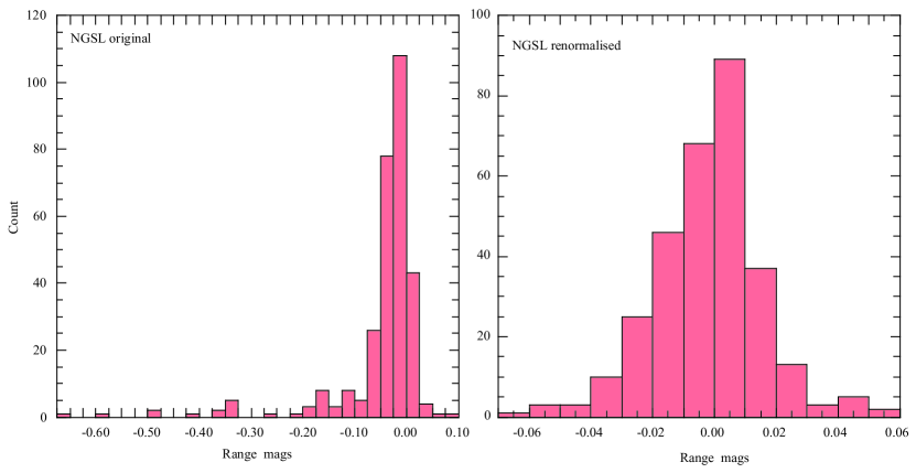
Figure 1: Histogram of difference between observed and synthetic $V$ magnitudes for original NGSL spectra (left) and renormalized spectra (right). The renormalized MILES spectra show a very similar distribution and rms.

The wavelength range of the NGSL spectra encompasses the wavelength range of the Hipparcos and Tycho passbands, but because the MILES spectra do not cover the complete extent of the red tails of the $H_{p}$ and the $R$ band, nor any of the $I$ band, we have extrapolated the MILES spectra from 7000Å  to 9900Å using model atmosphere fits to the 3500Å-7000Å region by Kerzendorf (2011). The grids used were from ATLAS (Munari et al., 2005) for $T_{eff}>$ 8000K and MARCS (Gustafsson et al., 2008) for 8000K$>T_{eff}>$ 2500K. The MILES spectra were also extrapolated from 3500Å to 3000Å to cover the $U$ band. These extrapolations may result in a slight uncertainty in the synthetic photometry in some passbands from the MILES spectra; however, we think that it is small, as shown by the insignificant differences between the relations using the NGSL and MILES spectra, except probably for the M stars.

The 373 adjusted NGSL spectrophotometric fluxes, covering the wavelength range 1800Å to 10100Å  and with a precise absolute flux level, are ideally suited to calibrate whole sky surveys, such as SkyMapper (Keller et al., 2007) and PanSTARRS (Kaiser et al., 2010). These revised absolute fluxes are available from the authors together with the absolute fluxes for the 836 MILES spectra that have Hipparcos photometry.

5 The $UBVRI$ passbands

The Johnson-Cousins $UBVRI$ system passbands have been well discussed (e.g. Azusienis & Straizys, 2009; Buser & Kurucz, 1978; Bessell, 1990a), most recently by Maiz Appellaniz (2006) who reconsidered the $UBV$ passbands. Although accepting the Bessell (1990a) $BV$ passbands, Maiz Appelaniz suggested an unusual and unphysical $U$ passband as providing a better fit to standard $U$ photometry. However, these previous analyses did not have available the large number of revised spectra in the NGSL and the MILES catalogs. It is very worthwhile, therefore, to reexamine the $UBVRI$ passbands using synthetic $UBVRI$ photometry derived from these extensive data sets. Standard system $UBV$ data for most of the MILES and NGSL stars are available in the homogenized $UBV$ catalog of (Mermilliod, 2006). $VI$ data are available for many stars in the Hipparcos catalog, while various data sets of Cousins, Menzies, Landolt, Bessell, Kilkenny and Koen also provided much supplementary $VRI$ data (Cousins, 1974, 1976, 1984; Cousins & Menzies, 1993; Landolt, 1983, 2009; Bessell, 1990b; Kilkenny et al., 1998; Koen et al., 2002, 2010) .

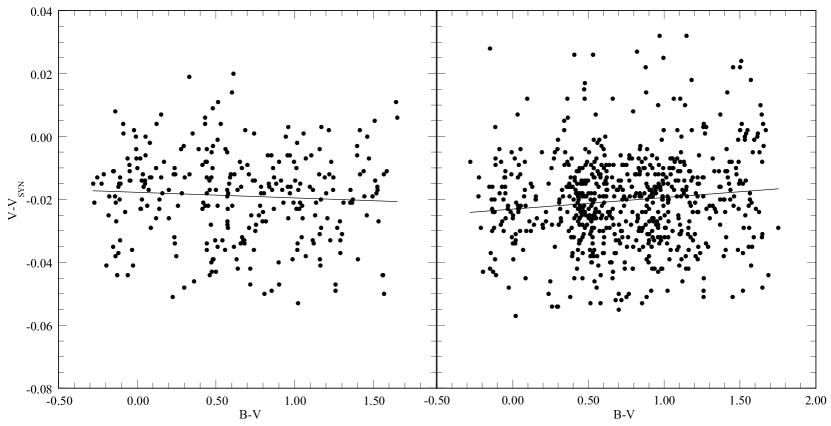
Figure 2: Difference between observed and synthetic $V$ magnitudes for NGSL (left) and MILES (right) samples. The solid lines show linear fits to the data.

5.1 The $B$ and $V$ passbands

After comparing the observed and synthetic photometry, very small slopes were evident in the $\Delta$ $B$ and $\Delta$ $V$ regressions against $B-V$ using the Bessell (1990a) passbands with the NGSL and MILES samples. These slopes were removed by making a small redward shift to the red side of the $V90$ band and a very small overall redward shift in the $B90$ band. The regressions for the MILES sample were similar but not identical. In Fig 2 and Fig 3 we show for the NGSL spectra the differences between the observed and synthetic $V$ and $B-V$, respectively, for our adopted passbands. There are no significant color terms evident, but the synthetic $V$ and $B-V$ mag scales have small apparent offsets associated with the initial adopted zero-points (hereinafter ZPs) of the synthetic photometry. These will be addressed further in Section 7.

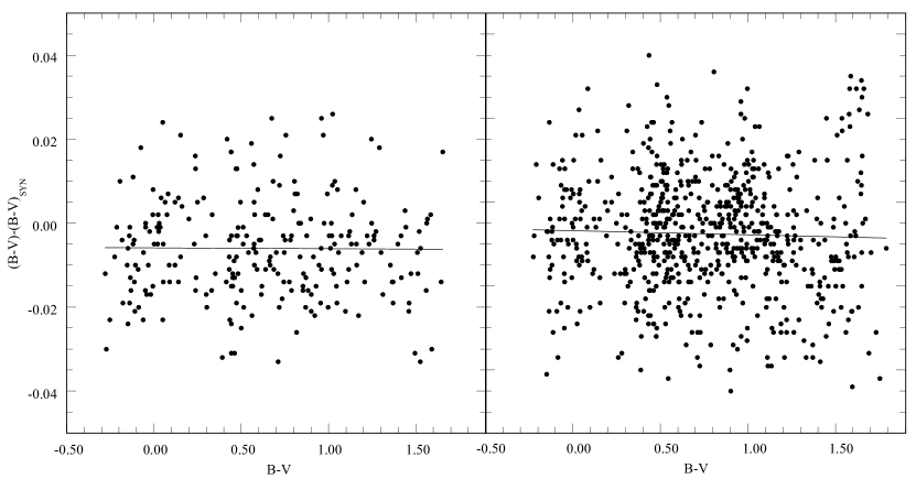
Figure 3: Difference between observed and synthetic $B-V$ for NGSL (left) and MILES (right) samples. The solid lines show linear fits to the data.

5.2 The $U$ bandpass revisited

Standard $U$ photometry has a bad reputation due to the much larger systematic differences in $U-B$ between observers than is evident for $V$ and $B-V$. These systematic differences arise because in stars, $U$ measures the flux across the region of the Balmer Jump and its response is therefore much more sensitive to the exact placement of the band compared to the placement of $B$ and $V$. Many observers take insufficient care to match the position and width of the standard Cousins or Johnson $U$ passband and attempts to standardize the resulting $U-B$ color using a single $B-V$ or $U-B$ color correction term have introduced systematic errors, especially for reddened stars. Cousins (1984) (reprised in Bessell, 1990a) outlined such systematic differences evident in different versions of the $U-B$ system.

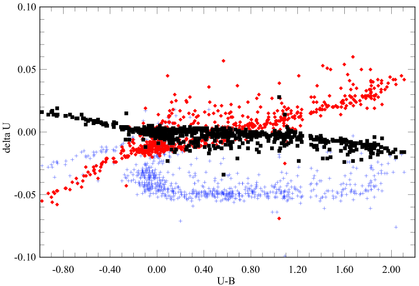
Figure 4: Differences in the MILES sample synthetic $U$mags computed with the $U$ passband in this paper and those of Bessell (1990a):$UX90$ (black squares), Buser & Kurucz (1978):U3 (red diamonds), Maiz Appellaniz (2006) (blue crosses).

Bessell (1986, 1990a) discussed in detail the likely response function of the $U$ band from first principles and proposed the $UX90$ band as representing the original band. Bessell, Castelli & Plez (1998, Appendix E3.1) note that the $U-B$ based on this band should be scaled by 0.96. Although scaling of this order is common in transforming observational systems (e.g. Menzies, 1993; Landolt, 1983), there is a notable reluctance to use such terms in computing synthetic photometry. In spite of the evidence that most standard systems have evolved with nonlinear or bi-linear correction terms (Bessell, Castelli & Plez, 1998, Appendix E1), most astronomers believe that a passband can be found that reproduces the standard system without the need for linear and/or nonlinear correction terms. In the spirit of that quixotic endeavour, Buser & Kurucz (1978) and Maiz Appellaniz (2006) proposed $U$ passbands that have almost identical red cutoffs to the $UX90$ band, but different UV cutoffs, thus shifting the effective wavelength of $U$ slightly redward. We have also produced a slightly different $U$ band by moving the UV cutoff of the $UX90$ band slightly redward. This produces an acceptable compromise for the $U$ band that fits the observations reasonably well, although a non-linear fit would be better.

In Fig 4, we show regressions against $U-B$ of the differences between the $U$ photometry synthesized with the passband from this paper and those of Bessell (1990a):$UX90$, Buser & Kurucz (1978):U3 and Maiz Appellaniz (2006). The main difference between Bessell (1990a) and Buser & Kurucz (1978) is a small difference in slope, whereas the Maiz Appellaniz (2006) passband mainly produces an offset of about 0.05 mag for G, K and M stars compared to the A and B stars.

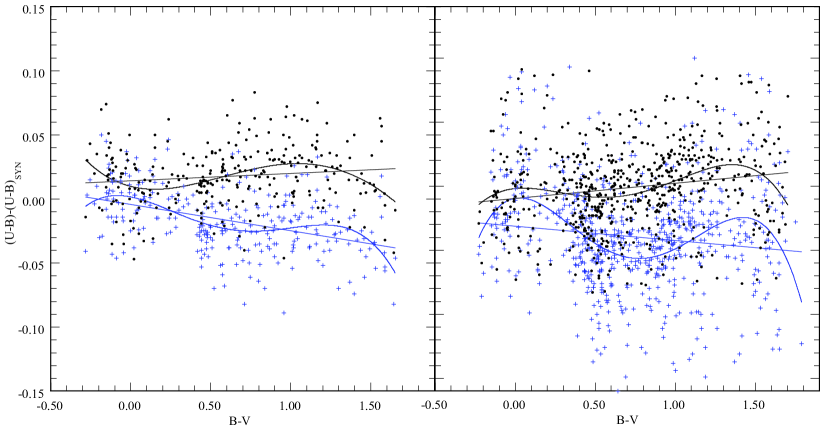
Figure 5: Differences between observed $U-B$ and synthetic $U-B$ for the NGSL (left) and MILES (right) sample of stars computed with the $U$ passband in this paper (black dots) and Maiz Appellaniz (2006) (blue crosses). The solid lines show the linear and 4th order fits to the differences.

In Fig 5, we show the differences between the observed values of $U-B$ and the synthetic $U-B$ computed for the NGSL and MILES sample of stars. Although the scatter is quite high, the Maiz Appellaniz (2006) $U$ passband clearly does less well and results in a systematic deviation from the standard system for the cooler stars (as anticipated in Fig 4).

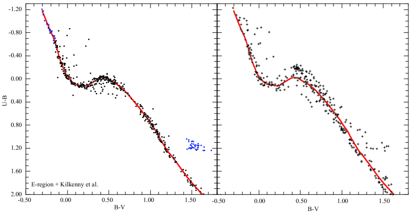
Figure 6: Left panel: standard $U-B$ versus $B-V$ relation; E-region stars (black dots), additional blue and red dwarfs (blue dots). Right panel: synthetic $U-B$ versus $B-V$ relation for adopted passbands and the NGSL stars. The thick red line is the same in both figures. The metal deficient stars in the NGSL sample lie above the red fiducial line for $B-V$ between 0.3 and 1.0

The SAAO $UBVRI$ photometry (Cousins, 1974, 1976; Kilkenny et al., 1998; Koen et al., 2002, 2010) represents some of the best standard $UBVRI$ photometry and we use the $U-B$ versus $B-V$ relation from these data (Fig 6 left panel) as the benchmark for comparison with the synthetic photometry. The Kilkenny et al. (1998) photometry (blue dots) extended the standard system to much bluer and redder dwarf stars than represented in the E-region stars (black dots). The red line is a fitted mean line through the O-B-A-F-G dwarf main sequence and the K & M giants. In the right panel of Fig 6, the same line is drawn for comparison on the synthetic $U-B$ versus $B-V$ diagram computed for the NGSL sample of stars using our adopted $UBV$ passbands. Considering that there are many metal-deficient F, G and K stars in the NGSL sample that are not in the empirical sample, the synthetic diagram is in good agreement with the empirical diagram. Note also that most of the reddest stars in the NGSL sample are K and M giants and there are only a few K and M dwarfs.

5.3 The $R$ and $I$ passbands

It was not as straightforward to check the $R$ and $I$ bands because of the lack of precise $RI$ photometry for many of the NGSL and MILES stars. The $V-I$ colors given in the Hipparcos catalog are of uncertain heritage, as are similar data from SIMBAD. An homogenized $VRI$ catalog would have been very useful. Our observational data comprised the Hipparcos $V-I$ color supplemented with $VRI$ data mostly from Bessell (1990b) and Koen et al. (2010) for the K and M dwarfs. Although the scatter was high for the Hipparcos $V-I$ comparison, it did indicate that a small shift in the Bessell (1990a) $I90$ band was needed. We eventually shifted the red edge of the $R90$ band a little redward and the whole $I90$ band a little blueward. In addition to the synthetic photometry from the NGSL and MILES samples, we also had available a small sample of unpublished single observations of mostly late-M dwarfs taken with the DBS at Siding Spring Observatory. As shown in Fig 7 , the resultant synthetic $V-R$ versus $V-I$ relations were in excellent agreement with the empirical loci defined by the precise values in Menzies et al. (1989), Menzies (1990), Landolt (2009), Bessell (1990b) and Koen et al. (2010). The four empirical data sets are essentially coincident. The sparse redder locus in the $V-R$ versus $V-I$ diagram beyond $V-I\sim 1.8$ are Landolt K and M giants. Note that this and later figures are best viewed magnified in the electronic version.

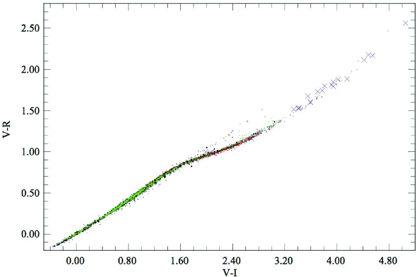
Figure 7: Comparison between empirical and synthetic $V-R$ versus $V-I$ relations. Empirical data: Landolt (2009) - blue dots; Koen et al. (2010) - red dots; Bessell (1990b) - dark green pluses. Synthetic data: NGSL - black squares; MILES - light green dots; Bessell 2007 M dwarf spectrophotometry - violet crosses.

To better appreciate the comparison we fitted a 9th order polynomial to the empirical $V-R$ versus $V-I$ locus and plotted the $V-R$ residuals of the fit against $V-I$. Applying the same polynomial, we also computed $V-R$ residuals for the synthetic photometry. In Fig 8 we overlay the synthetic residuals, which are seen to agree very well with the trends in the empirical residuals. The few hundredths of a mag systematic differences between the MILES $VRI$ colors for the M dwarfs compared to the empirical stars is undoubtedly due to the extrapolation of the MILES spectra from 7000Å to 9900Å using model spectra. However, for non-M stars, the relation defined by the extrapolated MILES spectra is indistinguishable from the others, indicating an impressive fidelity of the ATLAS (Munari et al., 2005) and MARCS (Gustafsson et al., 2008) spectra.

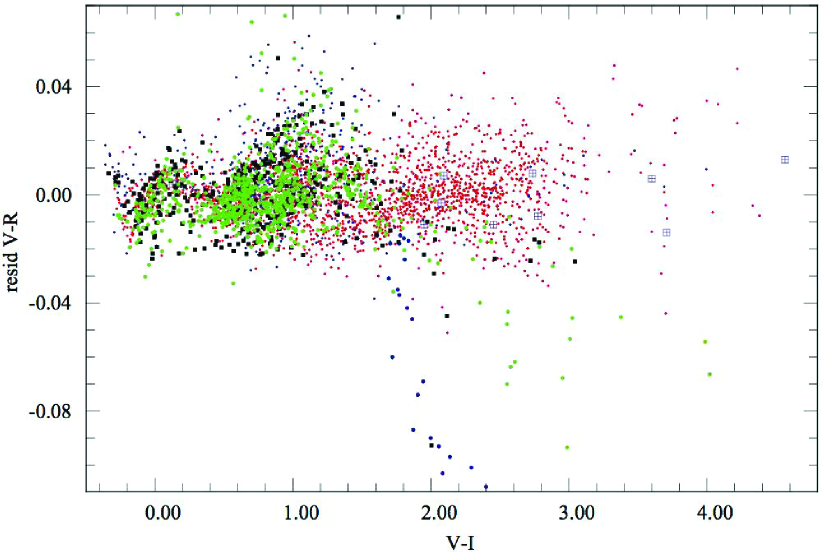
Figure 8: Comparison between the residuals of the same 9th order polynomial fit to the synthetic and catalog $V-R$ versus $V-I$ relations (see text for details). Synthetic photometry: NGSL - black squares; MILES - green dots; Bessell unpublished M dwarfs spectra - violet crossed boxes. Observed photometry: E-region stars (Menzies et al., 1989; Menzies, 1990) - red dots; K and M dwarfs (Koen et al., 2010; Bessell, 1990a) - red dots; Landolt (Landolt, 2009) dwarfs - blue dots, giants - larger blue dots.

5.4 Photometric passbands: photon counting and energy integrating response functions

There continues to be some confusion in the definition of photometric response functions and their use in computing synthetic photometry. As discussed in Koornneef et al. (1986), Appendix 4 of Bessell, Castelli & Plez (1998) and in Appendix A of Maiz Appellaniz (2006), in the era before CCDs, photometry was largely done with energy measuring detectors. The normalized response functions, $S^{\prime}_{x}(\lambda)$, that were generally published described the relative fraction of energy detected at different wavelengths across a particular passband. Nowadays, detectors are almost all photon integrating devices, such as CCDs, and the response functions used, $S_{x}(\lambda)$, relate to the relative number of photons detected (or the probability of a photon being detected) at different wavelengths across the passband. These issues are outlined and explored in the Appendix, where it is also shown why the magnitudes derived from photon counting or energy integration observations are identical (as expected). In Table 1 we list our adopted normalized photon-counting passbands $S_{x}(\lambda)$ for $U$, $B$, $V$, $R$ and $I$. In Fig 9 we show the normalized photon-counting passbands for $U$, $B$, $V$, $R$ and $I$ compared to the Bessell (1990a) passbands converted to photon-counting. The Maiz Appellaniz (2006) $U$ band and the converted Buser & Kurucz (1978) photon-counting $U3$ band are also shown.

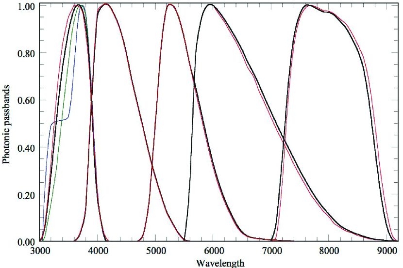
Figure 9: Photonic passbands (system response functions) $S_{x}(\lambda)$ for $UBVRI$. This paper - thick black; $U$: Maiz Appellaniz (2006) - blue; $U3$: Buser & Kurucz (1978) - green; Bessell (1990a) - red. See text for details.

6 Hipparcos $H_{p}$ and Tycho $B_{T}$ and $V_{T}$ passbands

There are two ground-based photometric systems notable for their precision and stability. These are the Walraven $VBLUW$ photometry of Pel & Lub (2007) and the $UBVRI$ SAAO and Landolt (2009) photometry discussed above. Pel (1990) also provided precise transformations between the Johnson-Cousins $V$ and $B-V$ and Walraven $V$ and $V-B$.

We regressed $V-H_{p}$, $B-B_{T}$ and $V-V_{T}$ versus $B-V$ for these two data sets and compared them with the synthetic photometry from the NGSL and MILES. As done for $UBV$, the $H_{p}$, $B_{T}$ and $V_{T}$ passbands were adjusted until the slopes and shapes of the regressions with the synthetic photometry matched as closely as possible those of the observed regressions. In order to remove the small color term evident in the initial regressions, the red side of the Bessell (2000) $V_{T}$ passband was shifted slightly redward while a smaller blueward shift was made to the blue side of the Bessell (2000) $B_{T}$ band. Fig 10 shows the final regressions for $B-B_{T}$ and $V-V_{T}$ from the NGSL spectra. Fig 11 shows the adopted $B_{T}$ and $V_{T}$ passbands in comparison to the original passbands (van Leeuwen et al., 1997a) and the Bessell (2000) passbands. There is little obvious difference between the three passbands. The adopted photon counting response functions for $B_{T}$ and $V_{T}$ are listed in Table 2.

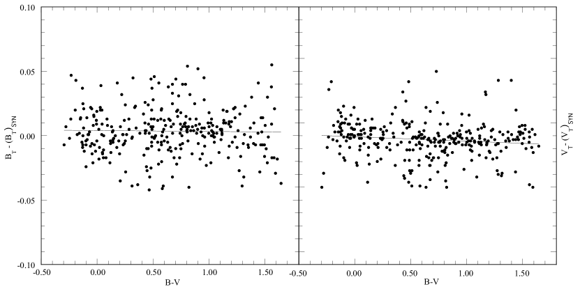
Figure 10: Differences between synthetic $B_{T}$, $V_{T}$ and catalog $B_{T}$, $V_{T}$ for the NGSL sample of stars.

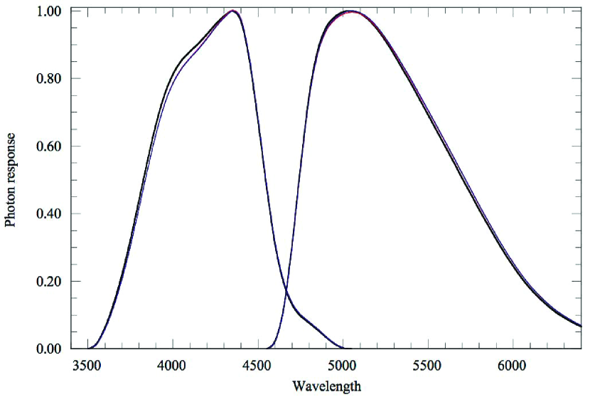
Figure 11: Photon-counting response functions $S_{x}(\lambda)$ for $B_{T}$ and $V_{T}$. This paper - thick black; van Leeuwen et al. (1997a) - blue; Bessell (1990a) - red.

There have been suggestions (e.g. Grenon, 2001), that the change in the $H_{p}$ sensitivity function caused by the in-orbit radiation damage was unlikely to be a complete loss of the bluest sensitivity as suggested by Bessell (2000), but rather a more complicated drop in sensitivity across a wider wavelength range. We have attempted to use the two spectrophotometric samples to examine this proposition and, whilst the results are not unequivocal, a slightly better fit is achieved by making small modifications to the Bessell (2000) passband.

The synthetic $V-H_{p}$ versus $U-B$ , $V-I$ and $B-V$ regressions are shown in Figs. 12, 13 and 14 respectively, in comparison with empirical relations for these stars. These plots show the range of stars represented in the NGSL spectrophotometric catalog (few K and M dwarfs but many FG subdwarfs) and the different distribution of stars in the comparison standard photometric SAAO catalogs. We have fitted a cubic polynomial to the $V-H_{p}$ versus $B-V$ regression for the E-region stars (Menzies et al., 1989; Menzies, 1990) bluer than $B-V$=1.1. The same polynomial in $B-V$ was applied to the catalog stars of Pel & Lub (2007); Pel (1990) and to the synthetic photometry of the NGSL and MILES stars.

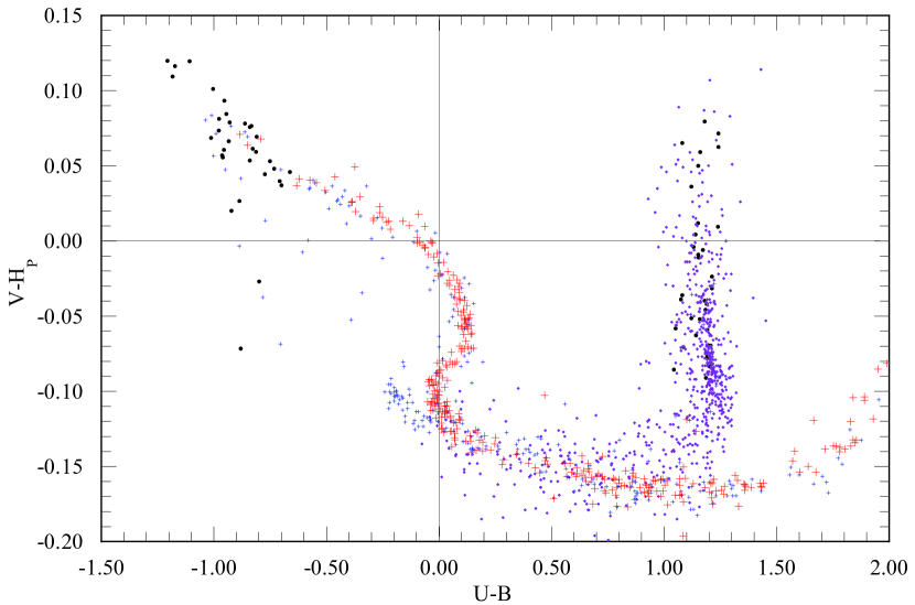
Figure 12: Comparison between synthetic and catalog $V-H_{P}$ versus $U-B$ relations. Synthetic: NGSL - blue. Observed: E-region stars - red; Kilkenny et al. (1998): more extreme O and B stars and M dwarfs - black dots; Koen et al. (2010): K and M Hipparcos dwarfs - violet. Note the large number of metal-deficient F and G stars in the NGSL sample with $U-B$ excesses and the very few K and M dwarfs in the NGSL sample. See text for details.

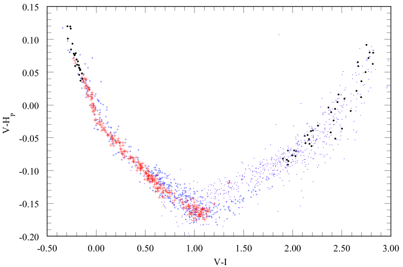
Figure 13: Comparison between synthetic and catalog $V-H_{P}$ versus $V-I$ relations. Synthetic: NGSL - blue. Observed: E-region stars - red; Kilkenny et al. (1998) - black; Koen et al. (2010) - violet. See text for details.

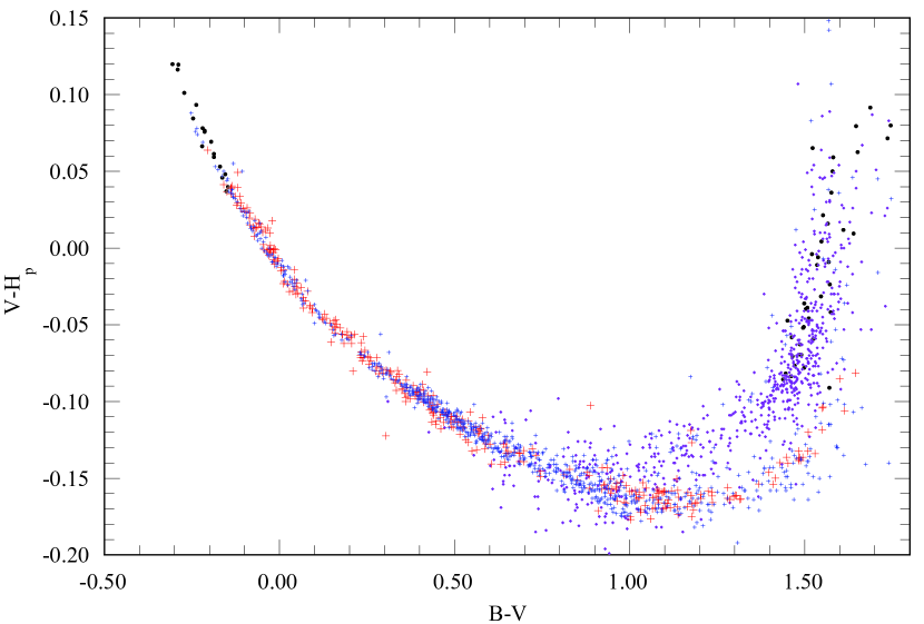
Figure 14: Comparison between synthetic and catalog $V-H_{P}$ versus $B-V$ relations. Synthetic: NGSL - blue. Observed: E-region stars - red; Kilkenny et al. (1998) - black; Koen et al. (2010) - violet. See text for details.

In Fig 15 we plot the residuals of the fit. It is clear that the synthetic photometry using the adopted $H_{p}$ band are a very good match to the standard photometry with the caveat that the ZPs of the synthetic $V-H_{p}$ mags were adjusted to achieve this. This will be discussed in the next section. Table 2 also lists the new Hipparcos passband while Fig 16 shows the new and old photon counting passbands.

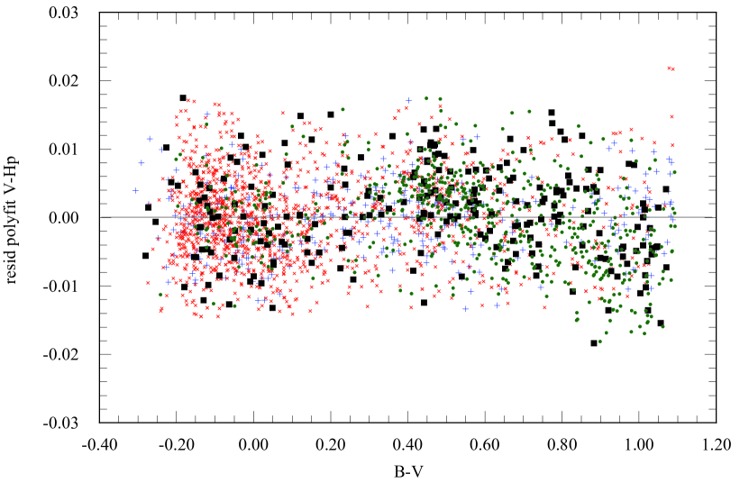
Figure 15: Comparison between the residuals of the same polynomial fit to the synthetic and catalog $V-H_{P}$ versus $B-V$ relations. Synthetic: NGSL - black squares; MILES - green dots. Observed: E-region stars Menzies et al. (1989), Menzies (1990) - red crosses; Pel & Lub (2007), Pel (1990) - blue pluses. See text for details.

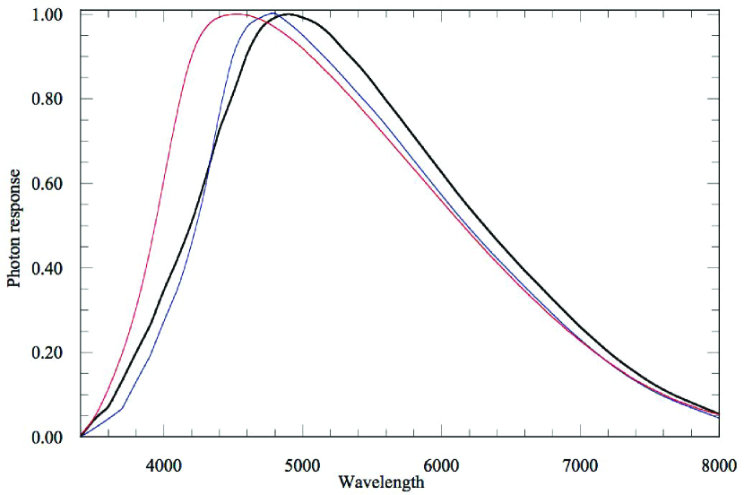
Figure 16: Photonic response functions $S(\lambda)$ for $H_{p}$. This paper - thick black; van Leeuwen et al. (1997a) - red; Bessell (1990a) - blue. See text for details.

7 $UBVRI$, $H_{p}$, $B_{T}$ and $V_{T}$ magnitudes and zero-points

All standard photometric systems adopt some ZP for their magnitude scale. Historically, the ZP of $V$ in the $UBV$ system is generally used for other systems.

The AB mag system (Oke & Gunn, 1983) (see Appendix) was defined as a monochromatic magnitude system for spectrophotometry where AB_ν = $-2.5$ log $f_{\nu}$ + 48.60 and $f_{\nu}$ is the flux in erg cm^-2 s^-1 Hz^-1. This has now been generalized for use with broad-band photometric bands. In the AB system, a flat spectrum star (in $f_{\nu}$) has the same AB magnitude in all passbands.

The AB_λ or ST mag system (see Appendix) was defined in terms of $f_{\lambda}$ where ST = $-2.5$ log $f_{\lambda}$ $+21.10$

The so-called VEGAMAG system (like the $UBV$ system) is one where Vega ($\alpha$ Lyrae) has colors (magnitude differences), such as $U-B$ and $B-V$, that are identically zero. This is equivalent to dividing all the observed fluxes by the flux of Vega but adjusting the $V$ ZP to give the adopted $V$ magnitude for Vega. For the Vega spectrum we used the CALSPEC (http://www.stsci.edu/hst/observatory/cdbs/calspec.html) spectrum alpha_lyr_stis_005, which is distributed in the synphot and pysynphot software packages (see Appendix).

7.1 Observed zero-points

The Hipparcos and Tycho magnitude ZPs (van Leeuwen et al., 1997b) were chosen to produce a VEGAMAG type system in which $H_{p}$ = $V_{T}$ = $V$ and $B_{T}$ = $B$ at $B-V$= 0, where $B$ and $V$ are standard magnitudes in the Johnson-Cousins $UBV$ system. Pel & Lub (2007) confirmed the excellent agreement between the $V$ magnitude scales of the homogenized $UBV$ system (Nicolet, 1978), the uvby system (Gronbech & Olsen, 1976; Olsen, 1983) the Hipparcos system and the Walraven $V,V-B$ system (Pel, 1990) (transformed with $V_{PL}$ = 6.886 $-2.5$$V_{W}$ $-$ 0.080($V_{W}-B_{W}$).

We have intercompared the Pel & Lub (2007) transformed $V_{PL}$ mags with those from the Hipparcos catalog (Perryman et al., 1997), the most recent homogenized $UBV$ catalog of Mermilliod (2006) and the E-region photometry from Menzies et al. (1989) and Menzies (1990). (We also derived $B-V$ = 2.539($V_{W}-B_{W}$) $-$ 0.827($V_{W}-B_{W})^{2}$ + 0.3121 ($V_{W}-B_{W})^{3}$ $-0.015$ from 1654 common stars in the Mermilliod (2006) homogenized $UBV$ catalog. The transformed $B-V$ values had an rms of 0.013 mag. A slightly different fit was obtained using SIMBAD $B-V$ values.) The results of the $V$ comparisons were $V_{Hip}=V_{PL}$ $-0.006$ (1523 stars); $V_{Merm}=V_{PL}$ $-0.005$ (1679 stars); the rms of these means are 0.0003 mag. The ZP differences are similar to the $V_{SAAO}\approx V_{PL}$ $-0.006$ reported by Cousins & Menzies (1993). We derived $V-H_{p}$ for the various observed samples and by fitting a cubic to the regressions against $B-V$ for $-0.3<B-V<$1.1 have determined the $V-H_{p}$ values for $B-V$=0. These are $-0.008$ (358 E-region stars), $-0.009$ (78 Landolt (2009) stars) and $-0.0003$ (1427 Pel & Lub (2007) stars). We also derived $V-V_{T}$ and $B-B_{T}$ and fitted polynomials to the $B-V$ regressions yielding $V-V_{T}$ ZPs of +0.002 (355 E- region stars)+0.008 (1618 Pel & Lub (2007) stars) and $B-B_{T}$ ZPs of $-0.003$ (367 E-region stars) and +0.002 (1708 Pel & Lub (2007) stars).

From these comparisons we confirm that Menzies et al. (1989), Menzies (1990), Landolt (2009) and Mermilliod (2006) have the same $V$mag ZP and that the transformed $V_{PL}$ mags (Pel, 1990) should be adjusted by $-0.006$ mag. (The original Walraven $VBLUW$ mags are unaffected.) Although the ZPs of the $H_{p}$, $V_{T}$ and $B_{T}$ systems need to be adjusted by $-0.008$, +0.002 and $-0.003$ mags, respectively, to put them on the same ZP as the $UBVRI$ system, we will retain the ZPs of the existing $H_{p}$, $B_{T}$ and $V_{T}$ systems defined by the Hipparcos and Tycho catalogs in this paper and derive synthetic photometry ZP corrections accordingly.

7.2 Synthetic photometry zero-points

We carried out synthetic photometry on the alpha_lyr_stis_005 spectrum and assigned ZPs to force $H_{p}$= $V_{T}$= $B_{T}$ = $U$= $B$ = 0.03 (see Appendix A1.1). These Vega-based f_ν and f_λ ZPs are listed in Table 3. All ZPs in this paper are to be subtracted from the AB mags (Equation 1).

Table 3: $UBVRI$ zero-points based on the STIS005 spectrum and $V$=0.03 for Vega

System	$U$	$B$	$V$	$R$	$I$	$B_{T}$	$V_{T}$	$H_{p}$
ABν = abmag	0.771	$-$0.138	$-$0.023	0.160	0.402	$-$0.090	$-$0.044	$-$0.022
ABλ = stmag	$-$0.142	$-$0.625	$-$0.019	0.538	1.220	$-$0.672	$-$0.115	$-$0.074
vegamag	$-$0.023	$-$0.023	$-$0.023	$-$0.023	$-$0.023	$-$0.023	$-$0.023	$-$0.023
$\lambda_{eff}$	3673	4368	5455	6426	7939	4215	5265	5188

With these ZPs we computed synthetic photometry for all NGSL and MILES stars that had Hipparcos photometry. The ZPs from the synthetic photometry will check (a) whether there are systematic differences between the mean MILES and NGSL flux calibrations and (b) whether the STIS005 spectrum correctly represents the empirical ZPs of the $UBVRI$ and $H_{p}$, $V_{T}$, and $B_{T}$ systems. We compared the synthetic magnitudes and/or colors with the observed magnitudes and colors and derived the mean differences. The few stars with exceptionally large differences were not used in the means. There were about 700 stars in the MILES sample and 300 stars in the NGSL sample. We also computed synthetic photometry for 46 of the CALSPEC spectra (http://www.stsci.edu/hst/observatory/cdbs/calspec.html), 27 of which have $UBVRI$ photometry from Landolt & Uomoto (2007) and Landolt (2009), 16 had $H_{p}$ photometry and 10 had Tycho photometry.

In Table 4 we list the mean differences. The standard errors of the means for the NGSL and MILES samples are less than 0.001 mag. There was good agreement between the NGSL and MILES $VR$ $I$, $V_{T}$ and $H_{p}$ results; however, the differences for $B$ and $B_{T}$ appear to be small but real. We chose to adopt the NGSL values for $B$ and $B_{T}$ in preference to the MILES values as the NGSL data were taken outside the atmosphere and are unaffected by atmospheric extinction. For the far fewer CALSPEC spectra, the errors in the mean were between 0.004 ($H_{p}$) and 0.04 ($B_{T}$ and $V_{T}$). Given the small number of CALSPEC stars with photometry, the mean differences in the colors of the much fainter CALSPEC spectra were in reasonable agreement with those for the NGSL sample, except for an unexplained difference of a few hundredths of a magnitude between the $V$ and H_p magnitudes.

Table 4: Mean differences between the synthetic and observed photometry

Source	$V$	$U-B$	$B-V$	$V-R$	$V-I$	$B_{T}$	$V_{T}$	$V-H_{p}$	Nstars
NGSL	0.002	$-$0.018	0.005	$\sim$0.0	0.004	$-$0.010	0.007	0.012	$\sim$300
MILES	0.004		$-$0.012	$\sim$0.0	$-$0.006	$-$0.032	0.007	0.012	$\sim$700

In Table 5 we list the additional ZP mag offsets that will place synthetic photometry computed with the AB mag ZPs from Table 3 on the same scale as the homogeneous $UBV$ system, the Cousins-Landolt $UBVRI$ system and the Hipparcos and Tycho systems. We also list two wavelengths associated with each passband, that are defined independently of the flux; the pivot wavelength, $\lambda{{}_{p}}$, and the mean photon wavelength $\lambda{{}_{0}}$ (see Appendix for details) and the FWHM of the passband; the wavelengths are given in Å. Note that these are the wavelengths that should be associated with published $UBVRI$ photometry, not the natural passbands used by various observers, as their photometry has been transformed onto the standard system.

Table 5: Adopted additional ZP magnitudes and passband parameters

	$U$	$B$	$V$	$R$	$I$	$B_{T}$	$V_{T}$	$H_{p}$
ZP	$-$0.010	0.008	0.003	0.003	0.002	$-$0.010	0.007	$-$0.008
$\Delta$$\lambda_{fwhm}$	625	890	830	1443	1499	718	962	2116
$\lambda_{p}$	3597	4377	5488	6515	7981	4190	5300	5347
$\lambda_{0}$	3603	4341	5499	6543	7994	4198	5315	5427

The uncertainties in these additional zero-points should only be a few milli-mags, except for $R$ and $I$ where it is more uncertain, as the available $V-I$ photometry was of lower precision.

Using these total ZP corrections we recomputed the mags for the Vega stis005 spectrum and obtained $V$ = 0.027, $U-B$ = 0.018, $B-V=-0.004$, $V-R$ = 0.000, $V-I=-0.001$. In addition, the 1994 ATLAS Vega spectrum of Castelli (http://wwwuser.oat.ts.astro.it/castelli/vega/fm05t9550g395k2odfnew.dat) gives $U-B=-0.017$, $B-V=-0.017$, $V-R=-0.004$, $V-I=-0.009$. For comparison, (Bessell, 1983) measured for Vega, $B-V=-0.01$, $V-R=-0.009$, $V-I=-0.005$.

8 Summary

Excellent spectrophotometric catalogs are now available from NGSL (Heap & Lindler, 2007, http://archive.stsci.edu/prepds/stisngsl/index.html) and MILES (Sanchez-Blazquez et al., 2006, http://www.iac.es/proyecto/miles/). In addition to their intrinsic worth, such stars are very useful to use to calibrate all-sky surveys, such as SkyMapper (Keller et al., 2007). However, the published absolute flux levels are imprecise or non-existent, so we have renormalized the spectra to their precise $H_{p}$ magnitudes. In order to do this it was necessary to determine the best $H_{p}$ passband. We also decided to reexamine the passbands representing the $UBVRI$ and Tycho $B_{T}$ and $V_{T}$ standard photometric systems using the renormalized NGSL and MILES spectra. We used the CALSPEC stis005 spectrum of Vega to derive the nominal ZP corrections to the AB mag fluxes and synthesized the various magnitudes and slightly adjusted the photonic passbands, achieving better agreement between the synthetic and standard magnitudes than possible with the previous passbands. In Table 1 and 2 we presented the adopted photonic passbands for $UBVRI$ and $H_{p}$, $B_{T}$ and $V_{T}$, respectively. Table 3 lists the ZP magnitude corrections based on the stis005 Vega spectrum and $V$ = 0.03.

We intercompared the ZPs of the $V$ magnitude scale of the SAAO Cousins-Landolt $UBVRI$ system, the homogenized Mermilliod (2006) $UBV$ system and the Walraven Pel & Lub (2007) system and the Hipparcos $H_{p}$ and Tycho $B_{T}$ and $V_{T}$ systems. We found small differences of less than 0.01 mag between them. The $H_{p}$ magnitude ZP differs by 0.008 mag from the ZP of the $UBVRI$ system.

We analysed the mean magnitude and color differences between the synthetic photometry and the standard photometry and proposed small additional ZP corrections to place the synthetic photometry computed using the AB mag ZPs in Table 3 onto the same ZPs as the standard system photometry. These additional ZP corrections are given in Table 5 together with the passband parameters that should be used to characterize the standard systems.

There was good agreement between the mean differences from the NGSL and MILES catalogs, although the mean level of the MILES blue fluxes deviated slightly, but systematically, from those of the NGSL spectra. The synthetic colors of the fainter CALSPEC spectra also supports the proposed additional ZP corrections except for an unexplained difference in the relative $V$ and $H_{p}$ magnitudes.

Finally, in the Appendix, we present an extensive discussion on the confusion in the literature concerning measured magnitudes, fluxes and response functions when broad-band photometry is involved and provided equations setting out clearly the derivation of photometric quantities. We also cross reference parameters and definitions used in the HST photometric packages synphot and its successor pysynphot. (Table A1).

Appendix A APPENDIX

There is unfortunately some confusion in the literature concerning measured magnitudes, fluxes and response functions when broad-band photometry is discussed. The definitions concerning monochromatic fluxes are clear – but see Soffer & Lynch (1999) concerning the paradoxes, errors, and confusions that arise when density distributions are involved – but the clarity is lost when these definitions are generalized to involve mean magnitudes, mean fluxes and the choice of the “effective” wavelength or frequency most appropriately associated with them.

A.1 Photometric quantities and definitions

In astronomy, flux ($f$) refers to the radiative flux density, a quantity in physics referred to as the spectral irradiance. In astronomy, flux is also referred to as the monochromatic flux $f_{\nu}$ or $f_{\lambda}$, to distinguish it from the total flux $F$ which is summed over all wavelengths or frequencies. In SI units, $f_{\lambda}$ is measured in W m^-3, or more practically in W m^-2 Å^-1, W m^-2 nm^-1 or W m^-2 $\mu$m^-1, depending on the part of the spectrum being considered. In cgs units it is measured in erg cm^-2 sec^-1 Å^-1, erg cm^-2 sec^-1 nm^-1 or erg cm^-2 sec^-1 $\mu$m^-1. (10³ erg cm^-2 sec^-1 = 1 W m^-2). In radio-astronomy, fluxes are usually expressed in terms of a non-SI unit, the flux unit or Jansky (Jy), which is equivalent to 10^-26 W m^-2 Hz^-1 or 10^-23 erg cm^-2 sec^-1 Hz^-1.

A good starting point for the relevant formulae and definitions used in photometry is Rufener & Nicolet (1988), Koornneef et al. (1986) and Tokunaga & Vacca (2005). The stellar flux is normally given in terms of $f_{\nu}$ or $f_{\lambda}$, and the units, respectively, are erg cm^-2 sec^-1 Hz^-1 and erg cm^-2 sec^-1 Å^-1 or in the SI system of units, W m^-2 Hz^-1 and W m^-2 nm^-1; although, rather than energy, the photon flux $n_{p}$ in photon m^-2 sec^-1 Hz^-1 or photon m^-2 sec^-1 Å^-1 is also used. The relations between these quantities are precisely defined for monochromatic light, namely

$f_{\nu}$ = f_λ$\dfrac{\lambda^{2}}{c}$

(A1)

and

$n_{p}$ = $f_{\lambda}$$\dfrac{\lambda}{hc}$

(A2)

The AB (absolute) magnitude scale was introduced by Oke (1965) who proposed the $f_{\nu}$ definition, having noted that a plot of $f_{\nu}$ versus 1/$\lambda$ for hot stars, was approximately linear in the optical part of the spectrum. The monochromatic magnitude AB was later defined by Oke & Gunn (1983) using the flux measurement adopted by Oke & Schild (1970) for Vega at 5480Å  and an apparent magnitude of $V$ = +0.035. The Vega flux was considered measured to an accuracy of about 2 percent. Oke & Schild (1970) measured the flux of Vega at a set of discrete 50Å bands. A mean value of $f_{\nu}$ = 3.46 $\times$ 10^-20 erg cm^-2 sec^-1 Hz^-1 or 3.36 $\times$ 10^-9 erg cm^-2 sec^-1 Å^-1 or 940 photon cm^-2 sec^-1 Å^-1 was measured at 5556Å. They then interpolated Vega’s flux to the value of 3.65 $\times$ 10^-20 erg cm^-2 sec^-1 Hz^-1 at 5480Å assumed to be the “effective” wavelength of the $V$ band and using this value together with $V$ = +0.035, derived the constant $-$48.60 associated with definition for the AB magnitude, namely

AB_ν = $-$2.5 log$f_{\nu}$ $-$ 48.60

(A3)

It is somewhat unfortunate that Oke chose to define the AB mag in terms of $f_{\nu}$ rather than $f_{\lambda}$, which is more appropriate for most stars; but the conversions, at least for monochromatic light, are straightforward.

AB_λ = $-$2.5 log$f_{\lambda}$ $-$ 21.10

(A4)

AB_λ is called STMAG in synphot and pysynphot. Note that these ZPs are based on the nominal wavelength of 5480Å for the $V$ band.

More recent measurements of Vega’s flux are about 2 percent brighter, and retaining the above values of the ZPs in the definition of AB mag and ST mag will mean that these scales will necessarily have different ZPs from the $V$ system. And if a different nominal wavelength for the $V$ band is adopted, this will introduce an additional systematic difference between the $f_{\nu}$ and $f_{\lambda}$ ZPs.

A.1.1 The flux and $V$ mag of Vega

Summaries of the direct measurements of the optical flux of Vega are given by Hayes (1985) and Megessier (1995), who proposed $f_{\lambda}$ = 3.44 $\pm$ 0.05 $\times$ 10^-9 and 3.46 $\pm$ 0.01 $\times$ 10^-9 erg cm^-2 sec^-1 Å^-1, respectively, for Vega at 5556Å. Cohen et al. (1992) adopted the Hayes value, together with the flux spectrum of a Vega ATLAS 9 model for their spectral irradiance calibration. More recently, Bohlin & Gilliland (2004) measured the flux for Vega using STIS spectra and Bohlin (2007) refined these observations and discussed model fits, including rapidly rotating pole-on models. Bohlin (2007) quoted an absolute flux at 5556Å  the same as Megessier (1995) and $V$ = 0.023 and adopted for Vega a combination of various source fluxes to produce the CALSPEC spectrum alpha_lyr_stis_005 that is now generally used by pysynphot and other routines.

Many direct $V$ measurements of Vega have been made over the years. An obvious problem has been its extreme brightness making it difficult to measure with sensitive photomultipliers on 1m telescopes; however, Bessell (1983) measured $V$ = 0.03 in comparison with Cousins bright equatorial stars using an Inconel coated 1% neutral density filter and a GaAs photomultiplier tube at Kitt Peak. This value is in exact agreement with Johnson et al. (1966). Hayes (1985) discussed measurements of the $V$ magnitude of Vega and discounted reports of its variability. More recently Gray (2007) also discussed observations of Vega. Mermilliod (2006) gives for Vega $V$ = 0.033 $\pm$0.012.

We have computed $V$ = 0.007 from the CALSPEC spectrum of Vega using our passband and the ZP of $-$48.60 in equation A3. This implies that ZPs of $-$48.58 and $-$21.08, respectively, would put the AB_ν and AB_λ mag scale on the same ZP as the $V$ mag system, but see Section 7.2 above.

A.2 Issues arising from a broad passband

Photometric observations are normally made by summing the flux over discrete wavelength intervals defined by a window (filter) function. A generalized filter function is a dimensionless (unitless) quantity $R$ representing the fraction of the flux $f$ at each wavelength, that is incident on the detector. It is the product of the atmospheric transmission, the mirror reflectivity, the optics transmission and the glass filter transmission. It is usually used in the form of a normalized function. The mean $f_{\lambda}$ flux would be expressed by the following equation

$\langle f_{\lambda}\rangle$ = $\frac{\displaystyle\int{f_{\lambda}(\lambda)R(\lambda)d\lambda}}{\displaystyle\int{R(\lambda)d\lambda}}$

(A5)

and a similar equation for $\langle f_{\nu}\rangle$ with all $\lambda$ replaced by $\nu$. All integrals are nominally from zero to infinity but are sensibly evaluated over the defined range of the filter passband.

One source of confusion is the fact that the flux is evaluated after the detector, not before it. This means that the filter function must be multiplied by the response function of the detector to give the system response function, as the detector converts the incident light into electrons, which are then amplified and measured. In the case of a photon counting detector, such as a CCD, the function $R$ is multiplied by the quantum efficiency $\eta$$(\lambda)$ of the CCD to give the system photon response function $S$. In the case of detectors with photocathodes using D.C. techniques and current integration, the function $R$ is multiplied by the photocathode radiant response $\sigma(\lambda)$ (in units of mA/W) to give the system energy response function $S^{\prime}$. Incorrect equations for photon counting and energy integration (e.g. Buser, 1986, equation 1 and 2) result from overlooking this difference. The system response functions are then generally renormalized.

The relations between $S(\lambda),S^{\prime}(\lambda)$, $\eta(\lambda)$ and $\sigma(\lambda)$ are

$$S(\lambda)=R(\lambda)\eta(\lambda)\quad\textrm{and}\quad S^{\prime}(\lambda)=R(\lambda)\sigma(\lambda)$$ (A6)

$\eta$$(\lambda)$ = $\dfrac{hc}{e\lambda}\sigma(\lambda)$ = $\dfrac{12.4}{\lambda}\sigma(\lambda)$, for $\lambda$ in Å , $\eta$ in percent and $\sigma$ in mA W^-1

(A7)

or

$\eta(\nu)$ = $\dfrac{h\nu}{e}\sigma_{\nu}(\nu)$

(A8)

Ignoring the atomic constants for the moment (and noting that the response functions are usually normalized) we can write

$S^{\prime}(\lambda)$ = $R(\lambda)\eta(\lambda)\lambda$ = $S(\lambda)\lambda$

(A9)

and

$S^{\prime}(\nu)$ = $R(\nu)\eta(\nu)/\nu$= $S(\nu)/\nu$

(A10)

So for an energy integrating detector we can express the measured mean energy flux as

$\langle f_{\lambda}\rangle$ = $\frac{\displaystyle\int{f_{\lambda}(\lambda)S^{\prime}(\lambda)d\lambda}}{\displaystyle\int{S^{\prime}(\lambda)d\lambda}}$ = $\frac{\displaystyle\int{f_{\lambda}(\lambda)S(\lambda)\lambda d\lambda}}{\displaystyle\int{S(\lambda)\lambda d\lambda}}$

(A11)

and for $\langle f_{\nu}\rangle$

$\langle f_{\nu}\rangle$ = $\frac{\displaystyle\int{f_{\nu}(\nu)S^{\prime}(\nu)d\nu}}{\displaystyle\int{S^{\prime}(\nu)d\nu}}$ = $\frac{\displaystyle\int{f_{\nu}(\nu)S(\nu)d\nu/\nu}}{\displaystyle\int{S(\nu)d\nu/\nu}}$= $\frac{\displaystyle\int{f_{\lambda}(\lambda)\dfrac{\lambda^{2}}{c}S(\lambda)\lambda\dfrac{c}{\lambda^{2}}d\lambda}}{\displaystyle\int{S(\lambda)\lambda\dfrac{c}{\lambda^{2}}d\lambda}}$ = $\frac{\displaystyle\int{f_{\lambda}(\lambda)S(\lambda)\lambda d\lambda}}{\displaystyle\int{S(\lambda)\dfrac{c}{\lambda}d\lambda}}$

(A12)

For photon-counting detectors, one electron is collected for every detected photon so the mean photon flux is given by

$\langle n_{p}\rangle$ = $\frac{\displaystyle\int{n_{p}(\lambda)S(\lambda)d\lambda}}{\displaystyle\int{S(\lambda)d\lambda}}$ = $\frac{\displaystyle\int{f_{\lambda}(\lambda)\dfrac{\lambda}{hc}S(\lambda)d\lambda}}{\displaystyle\int{\dfrac{\lambda}{hc}S(\lambda)d\lambda}}$ $\times$ $\frac{\displaystyle\int{S(\lambda)\dfrac{\lambda}{hc}d\lambda}}{\displaystyle\int{S(\lambda)d\lambda}}$ = $\langle f_{\lambda}\rangle$ $\dfrac{\lambda_{0}}{hc}$

(A13)

where

$\lambda_{0}$ = $\frac{\displaystyle\int{\lambda S(\lambda)d\lambda}}{\displaystyle\int{S(\lambda)d\lambda}}$

(A14)

Equation A13 is very important because it shows that in broad band photometry, the mean photon flux is proportional to the mean energy flux and counting photons is equivalent to integrating the energy. Furthermore, the wavelength $\lambda_{0}$ is the representative wavelength of the mean photons and could be called the mean photon wavelength of the passband.

A.2.1 Definitions of other wavelengths and frequencies associated with a passband

Now, because monochromatically $f_{\nu}$ = f${}_{\lambda}\dfrac{\lambda^{2}}{c}$ we can write that

$\langle f_{\nu}\rangle$ = $\langle f_{\lambda}\rangle$$\dfrac{\lambda_{p}^{2}}{c}$

(A15)

where $\lambda_{p}$ is called the pivot-wavelength and from equations A11 and A12 can be shown to be

$\lambda_{p}$ = $\sqrt{\frac{\displaystyle\int{S(\lambda)\lambda d\lambda}}{\displaystyle\int{\dfrac{S(\lambda)}{\lambda}d\lambda}}}$

(A16)

As noted by Koornneef et al. (1986), the pivot-wavelength is convenient because it allows an exact conversion between the mean broadband fluxes $\langle f_{\nu}\rangle$ and $\langle f_{\lambda}\rangle$.

We defined above the mean photon wavelength $\lambda_{0}$; we could also define the mean energy wavelength that is

$\lambda^{\prime}_{0}$ = $\frac{\displaystyle\int{\lambda S^{\prime}(\lambda)d\lambda}}{\displaystyle\int{S^{\prime}(\lambda)d\lambda}}$ = $\frac{\displaystyle\int{S(\lambda)\lambda^{2}d\lambda}}{\displaystyle\int{S(\lambda)\lambda d\lambda}}$

(A17)

This mean wavelength was discussed by King (1952) who cites it as being favoured by Stromgren and Wesselink as a flux independent “effective” wavelength for broad band systems.

Two other wavelengths are commonly used: the isophotal wavelength and the effective wavelength.

The isophotal wavelength $\lambda_{iso}$, recommended by Cohen et al. (1992), is the wavelength at which the interpolated, smoothed monochromatic flux has the same value as the mean flux integrated across the band. That is

$f_{\lambda}(\lambda_{iso})$ = $\langle f_{\lambda}\rangle$ = $\frac{\displaystyle\int{f_{\lambda}(\lambda)S^{\prime}(\lambda)d\lambda}}{\displaystyle\int{S^{\prime}(\lambda)d\lambda}}$ = $\frac{\displaystyle\int{f_{\lambda}(\lambda)S(\lambda)\lambda d\lambda}}{\displaystyle\int{S(\lambda)\lambda d\lambda}}$

(A18)

A similar expression can be written for the isophotal frequency.

$f_{\nu}(\nu_{iso})$ = $\langle f_{\nu}\rangle$ = $\frac{\displaystyle\int{f_{\nu}(\nu)S(\nu)/\nu d\nu}}{\displaystyle\int{S(\nu)/\nu d\nu}}$

(A19)

Note that both definitions relate to the energy flux but a different pair of equations could be defined in terms of the photon flux.

$n_{p}(\lambda_{iso})$ = $\langle n_{p}\rangle$ = $\frac{\displaystyle\int{n_{p}(\lambda)S(\lambda)d\lambda}}{\displaystyle\int{S(\lambda)d\lambda}}$ = $\dfrac{(1/hc)\displaystyle\int{f_{\lambda}(\lambda)S(\lambda)\lambda d\lambda}}{\displaystyle\int{S(\lambda)\lambda d\lambda}}$ $\times$ $\frac{\displaystyle\int{S(\lambda)\lambda d\lambda}}{\displaystyle\int{S(\lambda)d\lambda}}$ = $\langle f_{\lambda}\rangle$ $\dfrac{\lambda_{0}}{hc}$

(A20)

The effective wavelength is usually defined as the flux-weighted mean wavelength. In terms of photons:

$\lambda_{eff}$ = $\frac{\displaystyle\int{\lambda n_{p}(\lambda)S(\lambda)d\lambda}}{\displaystyle\int{n_{p}(\lambda)S(\lambda)d\lambda}}$ = $\frac{\displaystyle\int{\lambda^{2}f_{\lambda}(\lambda)S(\lambda)d\lambda}}{\displaystyle\int{\lambda f_{\lambda}(\lambda)S(\lambda)d\lambda}}$

(A21)

which is the same as in terms of energy:

$\lambda^{\prime}_{eff}$ = $\frac{\displaystyle\int{\lambda f_{\lambda}(\lambda)S^{\prime}(\lambda)d\lambda}}{\displaystyle\int{f_{\lambda}(\lambda)S^{\prime}(\lambda)d\lambda}}$ = $\frac{\displaystyle\int{\lambda^{2}f_{\lambda}(\lambda)S(\lambda)d\lambda}}{\displaystyle\int{f_{\lambda}(\lambda)S(\lambda)\lambda d\lambda}}$

(A22)

and

$\nu^{\prime}_{eff}$ = $\frac{\displaystyle\int{\nu f_{\nu}(\nu)S^{\prime}(\nu)d\nu}}{\displaystyle\int{f_{\nu}(\nu)S^{\prime}(\nu)d\nu}}$ = $\frac{\displaystyle\int{f_{\nu}(\nu)S(\nu)d\nu}}{\displaystyle\int{f_{\nu}(\nu)S(\nu)d\nu/\nu}}$

(A23)

Note that $\lambda_{iso}$ and $\lambda_{eff}$ depend explicitly on the underlying flux distribution through the filter.

The definitions and labels of the various wavelengths and frequencies have long stirred passions. King (1952) argued strongly against the currently accepted use of “effective wavelength” and “effective frequency” as defined in equations A22, A23 noting that the meaning of “effective wavelength” is better served by the isophotal wavelength. He further proposed that the mean wavelengths, defined in equations A14 and A17 to a first approximation, act as effective wavelengths for all stars, being independent of the flux distribution.

Finally, Schneider et al. (1983) for aesthetic reasons, defined the effective frequency for a passband to be

$\nu^{*}_{eff}$ = exp$\langle\text{ln }\nu\rangle$ = exp$\frac{\displaystyle\int{(\text{ln }\nu)n_{p}(\nu)S(\nu)d\nu}}{\displaystyle\int{n_{p}(\nu)S(\nu)d\nu}}$

(A24)

and it follows that

$\lambda^{*}_{eff}$ = exp$\langle\text{ln }\lambda\rangle$ = exp$\frac{\displaystyle\int{(\text{ln }\lambda)n_{p}(\nu)S(\nu)d\nu}}{\displaystyle\int{n_{p}(\nu)S(\nu)d\nu}}$ = exp$\frac{\displaystyle\int{(\text{ln }\lambda)f_{\nu}(\nu)S(\nu)(1/\nu)d\nu}}{\displaystyle\int{f_{\nu}(\nu)S(\nu)(1/\nu)d\nu}}$

= exp$\frac{\displaystyle\int{(\text{ln }\lambda)f_{\nu}(\nu)S(\nu)d(\text{ln }\nu)}}{\displaystyle\int{f_{\nu}(\nu)S(\nu)d(\text{ln }\nu)}}$

(A25)

We note that this is not what Fukugita et al. (1996) claimed Schneider et al. (1983) defined as $\lambda_{eff}$. Fukugita et al. (1996) defined

$\lambda_{eff}$ = exp$\langle\text{ln }\lambda\rangle$ = exp$\frac{\displaystyle\int{(\text{ln }\lambda)S(\nu)d(\text{ln }\nu)}}{\displaystyle\int{S(\nu)d(\text{ln }\nu)}}$

(A26)

which is not flux averaged as is the $\lambda_{eff}$ of Schneider et al. (1983). To further complicate definitions, Doi et al. (2010) defined

$\lambda_{eff}$ = $\dfrac{c}{\nu_{eff}}$

(A27)

where

$\nu_{eff}$ = $\frac{\displaystyle\int{\nu S(\nu)d\nu/h\nu}}{\displaystyle\int{S(\nu)d\nu/h\nu}}$ = $\frac{\displaystyle\int{\nu S^{\prime}(\nu)d\nu}}{\displaystyle\int{S^{\prime}(\nu)d\nu}}$

(A28)

Equation A28 is the definition of the mean energy-weighted frequency not the mean (effective [sic]) photon weighted frequency as stated by Doi et al. (2010). Footnote 13 in that paper is also in error.

The “effective” frequency defined by Doi et al. (2010) is the “mean” frequency defined by Koornneef et al. (1986) and not the usual definition of the flux-weighted “effective” frequency similar to the Schneider et al. (1983) “effective” frequency.

For comparison we evaluate the labelled wavelengths for the $V$ band and Vega. Some, such as $\lambda_{eff}$, involve the product of the stellar flux and the system response function, while others such as $\lambda_{p}$ and $\lambda_{0}$ concern the system response passband only. Some of the different labelled photon counting wavelength values are ($\lambda_{eff},\lambda_{iso},\lambda_{p}$) = (5455Å, 5486Å, 5488Å). The mean photon wavelength $\lambda_{0}$ = 5499Å compared with the mean energy wavelength $\lambda^{\prime}_{0}$ = 5524Å. The Schneider et al. (1983) $\lambda^{*}_{eff}$ = 5444Å, the Fukugita et al. (1996) $\lambda_{eff}$ = 5464Å and the Doi et al. (2010) $\lambda_{eff}$ = 5453Å. We have marked some of these wavelengths in Fig A1 showing the $f_{\nu}$ flux (in mags) of Vega between 5400Å and 5600Å.

This illustrates the unecessary confusion of these weighted wavelengths. We recommend the retention of only two, the pivot wavelength, $\lambda_{p}$, that is a property of the passband only, and the isophotal wavelength, $\lambda_{iso}$, that takes into account the spectrum measured. To better quantify the derivation of the isophotal wavelength, we recommend that the flux be smoothed to a resolution of 1/3rd of the FWHM of the passband. The pivot wavelength should be used as part of a description of the filter system, while the isophotal wavelength should be used to plot the fluxes as broadband magnitudes against wavelength.

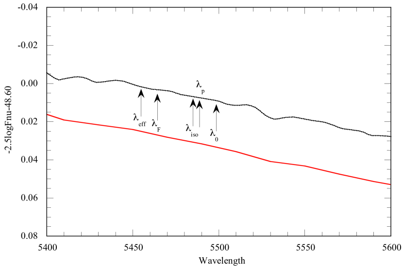
Figure A1: STIS005 $f_{\nu}$ spectrum of Vega (black) with some specific wavelengths marked (see text). $\lambda_{F}$ is Fukugita et al. (1996) $\lambda_{eff}$. The STIS005 spectrum yields $V$ = 0.007 mag. The red line is the Castelli 1994 Vega model flux scaled by $1.2876\times 10^{15}$ to produce $V$=0.03 mag.

A.2.2 Equations involving observed fluxes

Following Oke & Gunn (1983), Fukugita et al. (1996) and Doi et al. (2010) defined the broadband AB magnitude as

AB mag = $-$2.5 log$\langle f_{\nu}\rangle$ $-$48.60 = $-$2.5 log$\left(\frac{\displaystyle\int{f_{\nu}(\nu)S(\nu)d\nu/\nu}}{\displaystyle\int{S(\nu)d\nu/\nu}}\right)$ $-$ 48.60

(A29)

Fukugita et al. (1996) imply that this is a photon counting magnitude, however the above equation is the energy integration equation, (see equation A12; and as discussed above, based on the vega_STIS005 spectrum, the constant should be $-$48.577 to be on the same magnitude scale as the $V$ system for $V_{vega}$ = 0.03).

Equation A13 showed that photon counting and energy integration magnitudes were equivalent but with different offset constants that are subsumed in the standardisation process. That is, the apparent observed magnitude is usually defined as

$m_{j}$ = $C_{j}$ $-$ 2.5 log $\displaystyle\int{n_{p}(\lambda)S(\lambda)d\lambda}$ = $C^{\prime}_{j}$ $-$ 2.5 log $\displaystyle\int{f_{\lambda}(\lambda)S(\lambda)\lambda d\lambda}$

(A30)

with the constants $C_{j}$ or $C^{\prime}_{j}$ found from photometric standards. Note that the left hand integral describes photon counting while the right hand integral describes energy integration. The regular appearance of the (normalized) product $S(\lambda)\lambda$ in integrals pertaining to photometric magnitudes is often explained simply as wavelength weighting the response function to account for photon counting, however it is primarily a consequence of the modern practice of using the photon response functions rather than the energy response functions used in the past.

The most important reason for maintaining the contemporary practice of using photonic response functions is the fact that they are the default response functions in commonly used data reductions packages, such as synphot and pysynphot. All the passbands published in this paper are photonic passbands $S(\lambda)$.

A.2.3 Synphot and pysynphot

The HST photometry packages synphot and pysynphot (http://stsdas.stsci.edu/pysynphot/; http://stsdas.stsci.edu/stsci_python_epydoc/SynphotManual.pdf) are commonly used for planning HST observations and synthetic photometry. It is useful to relate the definitions, variable names and labels in these packages to those used in this paper. Table A1 is a cross-reference list of terms.

Table A1: Cross-reference of Photometric Terms

Equation	Name	Description	synphot	pysynphot
	$R$	pre-detector response function
A6	$S$	photon response function	$P_{\lambda}$	$P_{\lambda}$ = SpectralElement = bp
A9	$S^{\prime}$	energy response function	$\lambda P_{\lambda}$	$\lambda P_{\lambda}$
A14	$\lambda_{0}$	mean wavelength	avgwv	bp.avgwave
A16	$\lambda_{p}$	pivot wavelength	pivwv	bp.pivot
A21	$\lambda_{eff}$	effective wavelength	efflam	Observation.efflam
A25	$\lambda^{*}_{eff}$	Schneider et al. (1983) $\lambda_{eff}$	barlam
	$f_{\lambda}$	flambda	flam	Observation.effstim(’flam’)
	$f_{\nu}$	fnu	fnu	Observation.effstim(’fnu’)
A3	ABν	$-$2.5 log $\langle f_{\nu}\rangle$ $-$48.60	abmag	Observation.effstim(’abmag’)
A4	ABλ	$-$2.5 log $\langle f_{\lambda}\rangle$ $-$21.10	stmag	Observation.effstim(’stmag’)

Table 1: Normalized $UBVRI$ photonic responses

Wave	$U$	Wave	$B$	Wave	$V$	Wave	$R$	Wave	$I$
3000	0.000	3600	0.000	4700	0.000	5500	0.000	7000	0.000
3050	0.019	3700	0.031	4800	0.033	5600	0.247	7100	0.090
3100	0.068	3800	0.137	4900	0.176	5700	0.780	7200	0.356
3150	0.167	3900	0.584	5000	0.485	5800	0.942	7300	0.658
3200	0.278	4000	0.947	5100	0.811	5900	0.998	7400	0.865
3250	0.398	4100	1.000	5200	0.986	6000	1.000	7500	0.960
3300	0.522	4200	1.000	5300	1.000	6100	0.974	7600	1.000
3350	0.636	4300	0.957	5400	0.955	6200	0.940	7700	0.998
3400	0.735	4400	0.895	5500	0.865	6300	0.901	7800	0.985
3450	0.813	4500	0.802	5600	0.750	6400	0.859	7900	0.973
3500	0.885	4600	0.682	5700	0.656	6500	0.814	8000	0.970
3550	0.940	4700	0.577	5800	0.545	6600	0.760	8100	0.958
3600	0.980	4800	0.474	5900	0.434	6700	0.713	8200	0.932
3650	1.000	4900	0.369	6000	0.334	6800	0.662	8300	0.904
3700	1.000	5000	0.278	6100	0.249	6900	0.605	8400	0.860
3750	0.974	5100	0.198	6200	0.180	7000	0.551	8500	0.810
3800	0.918	5200	0.125	6300	0.124	7100	0.497	8600	0.734
3850	0.802	5300	0.078	6400	0.075	7200	0.446	8700	0.590
3900	0.590	5400	0.036	6500	0.041	7300	0.399	8800	0.392
3950	0.355	5500	0.008	6600	0.022	7400	0.350	8900	0.203
4000	0.194	5600	0.000	6700	0.014	7500	0.301	9000	0.070
4050	0.107			6800	0.011	7600	0.257	9100	0.008
4100	0.046			6900	0.008	7700	0.215	9200	0.000
4150	0.003			7000	0.006	7800	0.177
4200	0.000			7100	0.004	7900	0.144
				7200	0.002	8000	0.116
				7300	0.001	8100	0.089
				7400	0.000	8200	0.066
						8300	0.051
						8400	0.039
						8500	0.030
						8600	0.021
						8700	0.014
						8800	0.008
						8900	0.006
						9000	0.003
						9100	0.000

Table 2: Normalized $H_{p}$ $B_{T}$ $V_{T}$ photonic responses

Wave	$H_{p}$	Wave	$B_{T}$	Wave	$V_{T}$
3400	0.000	3500	0.000	4550	0.000
3500	0.041	3550	0.015	4600	0.023
3600	0.072	3600	0.063	4650	0.119
3700	0.133	3650	0.132	4700	0.308
3800	0.199	3700	0.220	4750	0.540
3900	0.263	3750	0.323	4800	0.749
4000	0.347	3800	0.439	4850	0.882
4100	0.423	3850	0.556	4900	0.951
4200	0.508	3900	0.664	4950	0.981
4300	0.612	3950	0.751	5000	0.997
4400	0.726	4000	0.813	5050	1.000
4500	0.813	4050	0.853	5100	0.992
4600	0.906	4100	0.880	5150	0.974
4700	0.966	4150	0.904	5200	0.946
4800	0.992	4200	0.931	5250	0.911
4900	1.000	4250	0.960	5300	0.870
5000	0.992	4300	0.984	5350	0.827
5100	0.978	4350	1.000	5400	0.784
5200	0.951	4400	0.969	5450	0.738
5300	0.914	4450	0.852	5500	0.692
5400	0.880	4500	0.674	5550	0.645
5500	0.840	4550	0.479	5600	0.599
5600	0.797	4600	0.309	5650	0.553
5700	0.755	4650	0.196	5700	0.504
5800	0.712	4700	0.131	5750	0.458
5900	0.668	4750	0.097	5800	0.412
6000	0.626	4800	0.077	5850	0.368
6100	0.583	4850	0.056	5900	0.324
6200	0.542	4900	0.035	5950	0.282
6300	0.503	4950	0.015	6000	0.245
6400	0.465	5000	0.003	6050	0.209
6500	0.429	5050	0.000	6100	0.178
6600	0.393			6150	0.152
6700	0.359			6200	0.129
6800	0.326			6250	0.108
6900	0.293			6300	0.092
7000	0.260			6350	0.078
7100	0.230			6400	0.066
7200	0.202			6450	0.055
7300	0.176			6500	0.044
7400	0.152			6550	0.036
7500	0.130			6600	0.027
7600	0.112			6650	0.017
7700	0.095			6700	0.008
7800	0.081			6750	0.000
7900	0.068
8000	0.054
8100	0.042
8200	0.032
8300	0.024
8400	0.018
8500	0.014
8600	0.010
8700	0.006
8800	0.002
8900	0.000

Facilities: HST: STIS; INT; SSO 2.3m: DBS

References

- Azusienis & Straizys (2009) Azusienis, A., & Straizys, V., 1969, SvA, 13, 316
- Abazajian et al. (2009) Abazajian, K.V. et al. 2009, ApJS, 182, 543
- Bessell (1983) Bessell, M.S., 1983 PASP, 95, 480
- Bessell (1986) Bessell, M.S., 1986, PASP, 98, 1303
- Bessell (1990a) Bessell, M.S., 1990a, PASP, 102, 1181
- Bessell (1990b) Bessell, M.S., 1990b, A&AS, 83, 357
- Bessell & Brett (1988) Bessell, MS, Brett, JM. 1988. PASP, 100, 1134
- Bessell, Castelli & Plez (1998) Bessell, M.S., Castelli, F., & Plez, B., A&A, 323, 231
- Bessell (2000) Bessell, M.S., 2000, PASP, 112, 961
- Bohlin & Gilliland (2004) Bohlin, R. C., & Gilliland, R. L. 2004, AJ, 127, 3508
- Bohlin (2007) Bohlin, R. C. 2007, in The Future of Photometric, Spectrophotometric, and Polarimetric Standardization, ASP Conf. Series, Vol. 364, p. 315 ed. C. Sterken
- Buser (1986) Buser, R., 1986, HiA, 7, 799
- Buser & Kurucz (1978) Buser, R., & Kurucz, R.L., 1978, A&A, 70, 555
- Cohen et al. (1992) Cohen, M., Walker, R.G., Barlow, M.J., & Deacon, J.R., 1992, AJ, 104, 1650
- Cousins (1974) Cousins, A. W. J. 1974, MNRAS, 166, 711
- Cousins (1976) Cousins, A.W.J., 1976, MmRAS, 81, 25
- Cousins (1984) Cousins, A.W.J., 1984, SAAOCirc, 8, 69
- Cousins & Menzies (1993) Cousins, A.W.J., Menzies, J.W., 1993, in Precision Photometry. Proceedings of a conference held to honour A.W.J. Cousins in his 90th year, held Observatory, Cape Town, South Africa, 2-3 February 1993. Edited by D. Kilkenny, E. Lastovica and J.W. Menzies. Cape Town: South African Astronomical Observatory (SAAO), p.240
- Doi et al. (2010) Doi, M., Tanaka, M., Fukugita, M., Gunn, J.E., Yasuda, N., Ivezic, Z., Brinkmann, J., de Haars, E., Kleinman, S.J., Krzesinski, J., French Leger, R., 2010, AJ,139, 1628
- Fukugita et al. (1996) Fukugita, M., Ichikawa, T., Gunn, J.E., Doi, M., Shimasaku, K., Schneider, D.P., 1996, AJ, 111, 1748
- Gray (2007) Gray, R. O. 2007, in The Future of Photometric, Spectrophotometric, and Polarimetric Standardization, ASP Conf. Series, Vol. 364, p. 305 ed. C. Sterken
- Grenon (2001) Grenon, M., 2001, private communication
- Gronbech & Olsen (1976) Gronbech, B., Olsen, E.H., 1976, A&AS, 34, 1
- Gustafsson et al. (2008) Gustafsson, B., Edvardsson, B., Eriksson, K., Jorgensen, U.G., Nordlund, A., Plez, B., 2008, A&A, 486, 951
- Hayes (1985) Hayes, D.S., 1985, In IAU Symposium 111: Calibration of fundamental stellar quantities, ed. D.S. Hayes, L.E. Pasinetti and A.G.Davis Philip, (Reidel: Dordrecht), p. 225
- Heap & Lindler (2007) Heap, S.R., & Lindler, D. 2007, IAUS, 241, 95
- Hog et al. (2000) Hog E., Fabricius C., Makarov V.V., Urban S., Corbin T., Wycoff G., Bastian U., Schwekendiek P., Wicenec A., “The Tycho2 catalogue”, 2000, A&A, 355, L27
- Johnson et al. (1966) Johnson, H.L., Iriarte, B., Mitchell, R.I., Wisniewskj, W.Z., 1966, CmLPL, 4, 99
- Kaiser et al. (2010) Kaiser, N, Burgett, W., Chambers, K., Denneau, L., Heasley, J., Jedicke, R., Magnier, E., Morgan, J., Onaka, P. & Tonry, J., 2010, SPIE 7733, 77330E1
- Keller et al. (2007) Keller, S. et al., 2007, PASA, 24, 1
- Kerzendorf (2011) Kerzendorf, W., 2011, private communication
- King (1952) King, I., 1952, ApJ, 115, 580
- Kilkenny et al. (1998) Kilkenny, D., van Wyk, F., Roberts, G., Marang, F., & Cooper, D., 1998, MNRAS, 294, 93
- Koen et al. (2002) Koen, C., Kilkenny, D., van Wyk, F., Cooper, D., & Marang, F., 2002, MNRAS, 334, 20
- Koen et al. (2010) Koen, C., Kilkenny, D., van Wyk, F., & Marang, F., 2010, MNRAS, 403, 1949
- Koornneef et al. (1986) Koornneef, J., Bohlin, R., Buser, R, Horne, K., Turnshek, D., 1986, HiA, 7, 833
- Landolt (1983) Landolt, A.U., 1983, AJ, 88, 439
- Landolt & Uomoto (2007) Landolt, A.U., Uomoto, A.K., 2007, AJ, 133, 768
- Landolt (2009) Landolt, A.U., 2009, AJ, 137, 4186
- Maiz Appellaniz (2006) Maiz Apellaniz, J., 2006, AJ, 131, 1184
- Megessier (1995) Megessier, C., 1995, A&A, 296, 771
- Menzies et al. (1989) Menzies, J. W., Cousins, A. W. J, Banfeld, R. M., & Laing, J. D., 1989, SAAO Circ., 13, 1
- Menzies (1990) Menzies, J. W., 1990, private communication
- Menzies (1993) Menzies, J.W., 1993, in Precision Photometry. Proceedings of a conference held to honour A.W.J. Cousins in his 90th year, held Observatory, Cape Town, South Africa, 2-3 February 1993. Edited by D. Kilkenny, E. Lastovica and J.W. Menzies. Cape Town: South African Astronomical Observatory (SAAO), p.35
- Mermilliod (2006) Mermilliod, J.C., 2006 Vizier II/168; Mermiliiod (1991) Universite de Lausanne.
- Munari et al. (2005) Munari, U., Sordo, R., Castelli, F., Zwitter, T., 2005, A&A, 442, 1127
- Nicolet (1978) Nicolet, B., 1978, A&AS, 34, 1
- Nicolet (1996) Nicolet, B. 1996. BaltA, 5, 417
- Olsen (1983) Olsen, E.H., 1983, A&AS, 54, 55
- Oke (1965) Oke, J.B., 1965, ARAA, 3, 23
- Oke & Schild (1970) Oke, J.B. & Schild, R., E. 1970, ApJ, 161, 1015
- Oke & Gunn (1983) Oke, J.B. & Gunn, J.E., 1983, ApJ, 266, 713
- Pel (1990) Pel, J-W., 1990, private communication
- Pel & Lub (2007) Pel, J-W.,& Lub, J., 2007, ASPConf, 364, 63
- Perryman et al. (1997) Perryman, M.A.C., Lindegren, L., Kovalevsky, J., Hog, E., Bastian, U., Bernacca, P.L., Creze, M., Donati, F., Grenon, M., Grewing, M., van Leeuwen, F., van der Marel, H., Mignard, F., Murray, C.A., Le Poole, R.S., Schrijver, H., Turon, C., Arenou, F., Froeschle, M., Petersen, C.S., “The Hipparcos Catalogue”, 1997,A&A,323,L49
- Rufener & Nicolet (1988) Rufener, F. & Nicolet, B., 1988, A&A, 206, 357
- Sanchez-Blazquez et al. (2006) Sanchez-Blazquez, P., Peletier, R. F., Jimenez-Vicente, J., Cardiel, N., Cenarro, A. J., Falcon-Barroso, J., Gorgas, J., Selam, S., Vazdekis, A., 2006,MNRAS,371,703
- Schneider et al. (1983) Schneider, D.P., Gunn, J.E., & Hoessel, J.G., 1983, ApJ, 264, 337
- Soffer & Lynch (1999) Soffer, B.H., & Lynch, D.K., 1999, AmJPhys, 67, 946
- Straižys (1996) Straižys, V. 1996. BaltA, 5, 459
- Straizys & Sviderskiene (1972) Straizys, V. & Sviderskiene, Z., 1972, Astron. Obs. Bull. Vilnius, 35, 1
- Tokunaga & Vacca (2005) Tokunaga, A.T., & Vacca, W.D., 2005, PASP, 117, 421
- van Leeuwen et al. (1997a) van Leeuwen, F., Lindegren, L., Mignard, F., 1997, The Hipparcos and Tycho Catalogues Vol. 3, ESA SP-1200, 461.
- van Leeuwen et al. (1997b) van Leeuwen, F., Evans, D. W., Grenon, M., Grossmann, V., Mignard, F., Perryman, M. A. C., 1997, A&A, 323, L61