Phenomenological Model for Predicting the Energy Resolution of Neutron-Damaged Coaxial HPGe Detectors

Abstract

The peak energy resolution of germanium detectors deteriorates with increasing neutron fluence. This is due to hole capture at neutron-created defects in the crystal which prevents the full energy of the gamma-ray from being recorded by the detector. A phenomenological model of coaxial HPGe detectors is developed that relies on a single, dimensionless parameter that is related to the probability for immediate trapping of a mobile hole in the damaged crystal. As this trap parameter is independent of detector dimensions and type, the model is useful for predicting energy resolution as a function of neutron fluence.

I Introduction

A gamma-ray traversing a germanium crystal loses energy mainly by the production of Compton electrons (or a photoelectron in the case of low-energy gamma-rays), which in turn lose energy by the production of electron-hole pairs at roughly 2.96 eV each. The electrons and holes are collected at the outer and inner electrodes covering the annular surfaces of the cylindrical crystal, thereby recording the energy of the gamma-ray. The full energy is not recovered, however, when holes are trapped at negatively charged defects in the crystal created by a flux of fast neutrons. Thus the energy resolution of gamma-ray peaks deteriorates with fast neutron fluence.

In practice, the gamma-ray energy is determined by measuring the current flow, induced by the moving electron and hole charges, between the electrodes. In this phenomenological model, the gamma-ray energy is instead calculated from the integrated charge at the two electrodes, induced by the electron-hole pairs.

This paper is laid out as follows. In section II the relation between an electron-hole pair and the induced charges at the electrodes is derived: this is essentially the concept of the detector. In section III expressions for the spatial density of hole traps (regions of fast neutron damage), and for the interaction cross-section of those traps, are derived. In anticipation of the computer implementation of the model, section IV describes the stochastic methods for choosing the location of electron-hole pair creation and subsequent location of the hole trapping. In section V the computer program, that combines these pieces of the model to produce spectral line peaks, is described. Finally, model results are compared to measurements, made in our laboratory, of the energy resolution of the 1332 keV ⁶⁰Co spectral line obtained by a p-type detector irradiated by a fast neutron fluence up to 10⁹ cm^-2.

The primary purpose of this work is to produce a predictive model of peak energy resolution as a function of fast neutron fluence. It is a phenomenological model, meaning that critical parameters are taken from experiment rather than calculated from first principles. The (dimensionless) critical parameters in this case are $\alpha_{h}$, which is related to the hole trap cross-section, and $\alpha_{t}$, which is essentially the average number of hole traps created by a fast neutron as it collides with atoms in the germanium crystal. (These are both introduced in section III.) Values for these parameters are obtained by reproducing, with the model, the data of R. H. Pehl et al. [1]. In that work, two HPGe coaxial detectors (one n-type, the other p-type), fabricated from the same crystal, were irradiated simultaneously with fast neutrons from an unmoderated ²⁵²Cf source.

For the convenience of the reader, SI units (and derived units) are used in any calculations: electric potential $\phi$ in volts (V); electric field $E$ in V$\cdot$m^-1; force in newtons (n); charge in coulombs (C). Note that 1 V = 1 n$\cdot$m$\cdot$C^-1. Further, the product $e$ ($v$ V) = $v$ eV. The electric charge $e=1.602\times 10^{-19}$ C; the vacuum permittivity $\epsilon_{0}=8.854\times 10^{-12}$ C${}^{2}\cdot$n${}^{-1}\cdot$m^-2.

Where the symbols $\pm$ and $\mp$ occur, the top/bottom sign is used for p-type/n-type detectors. The coaxial detector is an annular cylinder so it is natural to use cylindrical coordinates $\left(r,z\right)$: the radius of the inner electrode is $R_{0}$; the radius of the outer electrode is $R_{1}$; the axial coordinate $z=0$ at the top of the coaxial detector (the end pointing at the radiation source), and $z>0$ within the detector.

II Induced charge at the electrodes due to electron-hole pairs

As an electron and hole have opposite charge, it is not until they move apart under the influence of the driving force $q\mathbf{E}$($r$) that charge is induced at the electrodes. The variable $q$ is the charge of the particle (so equals $+e$/$-e$ for holes/electrons) and $\mathbf{E}(r)$ is the electric field at the particle location $r$ between the electrodes. In the case of p-type detectors, the outer contact is positively biased so that the field $\mathbf{E}(r)$ is negative; thus holes move towards the inner contact at $R_{0}$ and electrons move towards the outer contact at $R_{1}$. In the case of n-type detectors, the inner contact is positively biased so that the field $\mathbf{E}(r)$ is positive; thus holes/electrons move towards the outer/inner contact.

What charges are induced at the electrodes by an electron-hole pair after separation? Expressions for these are easily found by use of Green’s reciprocation theorem [2]: For a given arrangement of electrodes, if $\phi$ is the potential due to a volume-charge distribution $\rho$ and a surface-charge distribution $\sigma$, while $\phi^{\prime}$ is the potential due to other charge distributions $\rho^{\prime}$ and $\sigma^{\prime}$, then

$$\int\nolimits_{V}\rho\phi^{\prime}d^{3}x+\int\nolimits_{S}\sigma\phi^{\prime}da=\int\nolimits_{V}\rho^{\prime}\phi d^{3}x+\int\nolimits_{S}\sigma^{\prime}\phi da\text{.}$$ (1)

In the “primed” system, set $\rho^{\prime}=\sigma^{\prime}=0$, so $\phi^{\prime}(r)$ is the solution to Laplace’s equation in cylindrical coordinates with boundary conditions $\phi^{\prime}=1$ at surface $S$, which is inner contact $R_{0}$, and $\phi^{\prime}=0$ at outer contact $R_{1}$. Then the right hand side equals zero, so the “unprimed” system (which is the annular cylinder with a point charge at $r$ and a surface charge at the inner contact) obeys the relation

$$\int\nolimits_{V}\rho\phi^{\prime}d^{3}x=-\int\nolimits_{S}\sigma da\text{.}$$ (2)

Recognizing that $\rho$ (the charged particle at $r$) is $q$ times the delta function produces the relation $q\phi^{\prime}(r)=-\int\nolimits_{S}\sigma da$. Thus the induced charge at the inner contact due to a charged particle at $r$ is

$$Q_{0}(r) =-q\phi^{\prime}(r)$$

$$=-q\left(1-\frac{\ln\left[r/R_{0}\right]}{\ln\left[R_{1}/R_{0}\right]}\right)=-q\frac{\ln\left[R_{1}/r\right]}{\ln\left[R_{1}/R_{0}\right]}\text{.}$$ (3)

Similarly (but setting $\phi^{\prime}=1$ at surface $S$, which is outer contact $R_{1}$, and $\phi^{\prime}=0$ at inner contact $R_{0}$), the induced charge $Q_{1}(r)$ at the outer contact due to a charged particle at $r$ is

$$Q_{1}(r)=-q\phi^{\prime}(r)=-q\frac{\ln\left[r/R_{0}\right]}{\ln\left[R_{1}/R_{0}\right]}\text{.}$$ (4)

Note that the induced charges $Q_{0}(r)$ and $Q_{1}(r)$ at the two electrodes are opposite in sign to the charge $q$ of the particle at $r$, and that the sum $Q_{0}(r)+Q_{1}(r)$ always equals $-q$.

Now consider an electron-hole pair created at $r_{i}$. As the two particles are of opposite sign and both reside at $r_{i}$, no charge is induced at the two contacts. However, as the two mobile charges separate and move radially to $r_{e}$ and $r_{h}$, respectively, the charge $Q_{0}$ is induced at the $R_{0}$ contact and the charge $Q_{1}$ is induced at the $R_{1}$ contact, where

$$Q_{0}=Q_{0}(r_{e})+Q_{0}(r_{h})=e\frac{\ln\left[r_{h}/r_{e}\right]}{\ln\left[R_{1}/R_{0}\right]}$$ (5)

$$Q_{1}=Q_{1}(r_{e})+Q_{1}(r_{h})=-e\frac{\ln\left[r_{h}/r_{e}\right]}{\ln\left[R_{1}/R_{0}\right]}\text{.}$$ (6)

It is these induced charges $Q_{0}$ and $Q_{1}$ that account for the current between the two contacts due to an electron-hole pair (note that an incremental change $\delta Q_{0}=-\delta Q_{1}$ always, as electric charge flows from one contact to the other). Note that initially $r_{e}=r_{h}=r_{i}$ so the induced charges $Q_{0}=Q_{1}=0$, and that when both mobile charges successfully reach their respective contacts, the induced charges $Q_{0}=\mp e$ and $Q_{1}=\pm e$, as expected (top/bottom sign indicates p-type/n-type detector). As the current between electrodes is just the transfer of charge from one to the other, the result $\left|Q_{0}\right|=\left|Q_{1}\right|=e$ allows the full creation energy of the electron-hole pair to be recorded.

For a p-type detector, when the hole is trapped at $r_{h}$ but the electron successfully reaches $R_{1}$, the charge induced at the central contact is $Q_{0}=-e\frac{\ln\left[R_{1}/r_{h}\right]}{\ln\left[R_{1}/R_{0}\right]}$ and the charge induced at the outer contact is $Q_{1}=e\frac{\ln\left[R_{1}/r_{h}\right]}{\ln\left[R_{1}/R_{0}\right]}$. Note that in this case $Q_{0}=Q_{0}\left(r_{h}\right)$ and $Q_{1}=e+Q_{1}\left(r_{h}\right)<e$, meaning that $\left|Q_{0}\right|=\left|Q_{1}\right|<e$ so not all of the pair creation energy is recorded. For an n-type detector, when the hole is trapped at $r_{h}$ but the electron successfully reaches $R_{0}$, the induced charges are $Q_{0}=e\frac{\ln\left[r_{h}/R_{0}\right]}{\ln\left[R_{1}/R_{0}\right]}$ and $Q_{1}=-e\frac{\ln\left[r_{h}/R_{0}\right]}{\ln\left[R_{1}/R_{0}\right]}$, and again not all of the pair creation energy is recorded. By examining the two expressions for $Q_{0}$ (or $Q_{1}$), it is evident that in general the average value $\left\langle\left|Q_{0}\right|\right\rangle$ for a damaged p-type detector will be less than that for a damaged n-type detector, since a spatially uniform flux of gamma-rays will produce more electron-hole pairs near the outer contact than near the inner contact, so resulting in more hole trapping near the outer contact (thus $\left\langle\ln\left[R_{1}/r_{h}\right]\right\rangle<\left\langle\ln\left[r_{h}/R_{0}\right]\right\rangle$). This effect translates into less energy being attributed to an incident gamma-ray by a p-type detector than by an n-type detector.

The induced charges (currents) at the contacts are related to the energy of the incident gamma-ray in a straightforward way. When the electron and hole reach their terminal locations at $r_{e}$ and $r_{h}$, respectively, the induced charges $Q_{0}$ and $Q_{1}$ correspond to an energy $\frac{Q}{e}\epsilon$ recorded by the detector, where $Q\equiv\left|Q_{0}\right|=\left|Q_{1}\right|$ and $\epsilon$ is the average energy needed to create an electron-hole pair (this is the energy needed to elevate an electron in the valence band into the conduction band). For germanium, $\epsilon=2.96$ eV at 77 K [3]. An incident gamma-ray of energy $E_{\gamma}$ that produces $n$ electron-hole pairs will thus record an energy $n\frac{\left\langle Q\right\rangle}{e}\epsilon$, where the average value $\left\langle Q\right\rangle$ is taken over all the $n$ pairs.

In the implementation of this model in a computer code, a value for $n$ is chosen for each incident gamma-ray from the Gaussian distribution $p(n)=\left(2\pi\sigma^{2}\right)^{-1/2}\exp\left[-\left(n-n_{\gamma}\right)^{2}/\left(2\sigma^{2}\right)\right]$. The average value $n_{\gamma}=E_{\gamma}/\epsilon$ [so for example, the $1332$ keV ⁶⁰Co gamma-ray produces (on average) $n_{\gamma}=4.5\times 10^{5}$ electron-hole pairs in a germanium detector]. The variance $\sigma^{2}=F\cdot n_{\gamma}$ where $F$ is the Fano factor (and is approximately $0.13$ for Ge detectors [3]). To obtain values for $n$ from this distribution, it is most convenient to use the Box-Muller method [4]: Consider the “standard normal” distribution $\phi(\nu)=\left(2\pi\right)^{-1/2}\exp\left[-\nu^{2}/2\right]$. Then the two random variables $\nu_{1}$ and $\nu_{2}$ will both have the standard normal distribution and will be independent, where

$$\nu_{1}=\left(-2\ln x_{1}\right)^{1/2}\cos\left(2\pi x_{2}\right)$$ (7)

$$\nu_{2}=\left(-2\ln x_{1}\right)^{1/2}\sin\left(2\pi x_{2}\right)$$ (8)

and $x_{1}$ and $x_{2}$ are random numbers taken from the uniform distribution on $(0,1]$. Then the desired value $n=n_{\gamma}+\sigma\nu$, where $\nu$ is either $\nu_{1}$ or $\nu_{2}$ calculated from Eq. (7) or Eq. (8).

Note that the FWHM of the Gaussian distribution $p(n)$ is $2\left(2\sigma^{2}\ln 2\right)^{1/2}$. The FWHM of the corresponding energy peak is then $2\left(2Fn_{\gamma}\ln 2\right)^{1/2}\cdot\epsilon=2\left(2FE_{\gamma}\epsilon\ln 2\right)^{1/2}$. So for example, in the absence of neutron damage, the FWHM of the peak corresponding to the $1332$ keV ⁶⁰Co spectral line is $1.686$ keV, while that of the peak corresponding to the $122.1$ keV ⁵⁷Co spectral line is $0.510$ keV.

III Hole trapping

The fate of mobile holes (and electrons) in the neutron-damaged crystal is determined by the spatial distribution of traps, and the trap cross-section. These two functions are derived in turn.

The distribution of particle traps should be uniform over a z-slice (thickness $dz$), since the source of gamma-rays (at which the detector is pointed) also acts as the primary source of neutrons. What then is the trap density $\rho_{q}(z)$ (the number of traps in the infinitesimal volume $A\cdot dz$ at axial position $z$, where $A$ is the cross-sectional area of the crystal)? Consider that the mean free path of an incident neutron is $l$. That is, the probability that the neutron first collides a distance $\left[z,z+dz\right]$ from its entry point into the crystal is $\exp\left[-z/l\right]\cdot\left(dz/l\right)$. Then $N\exp\left[-z/l\right]\cdot\left(dz/l\right)$ is the number of neutrons that first collide a distance $\left[z,z+dz\right]$ from their entry point at $z=0$, where $N$ is the number of neutrons incident on the crystal. Assuming that the collision produces a trap, the trap density

$$\rho_{q}(z) =\alpha_{t}\cdot N\exp\left[-z/l\right]\cdot\left(dz/l\right)/\left(A\cdot dz\right)$$

$$=\alpha_{t}\cdot\frac{N}{lA}\exp\left[-z/l\right]$$ (9)

where $N/A$ is the neutron fluence, and the dimensionless parameter $\alpha_{t}$ is the (average) number of traps created by a fast neutron as it collides with atoms in the germanium crystal. Note that $\alpha_{t}$ should be somewhat larger than $1$, to account—in a crude way—for any subsequent collisions by the neutron.

What is a reasonable value for $\alpha_{t}$? For a neutron incident on a detector of length (thickness) $L$, the probability that no collisions occur over the distance $L$ is $\exp\left[-L/l\right]$, meaning that for a neutron fluence $N/A$, the fraction $1-\exp\left[-L/l\right]$ undergo at least one collision. L. S. Darken et al. [5], after irradiating a $3$ cm thick Ge crystal with neutrons, conclude “A fast neutron flux of $10^{10}$ cm^-2 produces about $2\times 10^{9}$ cm^-3 disordered regions of various sizes”. Setting $l=6$ cm [6] and $L=3$ cm, the fraction of incident neutrons that underwent collisions in the crystal was $0.3935$. Each of those neutrons was then responsible for $\left(2\times 10^{9}\times 3\right)/\left(0.3935\times 10^{10}\right)=1.5$ traps per (collided) neutrons. Thus in general $\alpha_{t}\sim 1.5$.

As charged particles, holes and electrons may be trapped at defects with opposite charge. It is believed that hole traps are large disordered regions with large negative charge [7], and so have a large effective cross-section, while electron traps are much smaller (perhaps point defects) and so have a much smaller cross-section. In any event, the trap cross-section $\sigma_{q}$ must be roughly the size of the local distortion, due to the electric charge of the defect, of the applied electric field $\mathbf{E}(r)$. An expression for $\sigma_{q}$ can be derived as follows.

For simplicity, use 2D Cartesian coordinates, and place the defect (with charge $Q$) at the origin, and set the no-defect electric field $\mathbf{E}=E\widehat{\mathbf{x}}$. Then the potential $\phi^{\ast}(\mathbf{r})$ at the point $\mathbf{r}=(x,y)$ for this system is $\phi\left(x\right)+\frac{Q}{\epsilon}\left(x^{2}+y^{2}\right)^{-1/2}$ where $\phi\left(x\right)$ is the potential at $\mathbf{r}$ in the absence of the defect and $\epsilon$ is the permittivity of germanium. This produces the electric field

$$\mathbf{E}^{\ast}\left(\mathbf{r}\right) =-\mathbf{\nabla}\phi^{\ast}\left(\mathbf{r}\right)=\left\{E+\frac{Q}{\epsilon}x\left(x^{2}+y^{2}\right)^{-3/2}\right\}\widehat{\mathbf{x}}$$

$$+\frac{Q}{\epsilon}y\left(x^{2}+y^{2}\right)^{-3/2}\widehat{\mathbf{y}}\text{.}$$ (10)

The electric field lines in the absence of the defect are directed parallel to the x-axis; in the presence of the charged defect at the origin, they are bent towards the origin. Those field lines that terminate at the defect are particle paths that lead to trapping. Clearly the field lines are seriously bent towards the defect when the magnitude of the y-component $\frac{Q}{\epsilon}y\left(x^{2}+y^{2}\right)^{-3/2}$ of the field $\mathbf{E}^{\ast}\left(\mathbf{r}\right)$ exceeds that of the x-component $E+\frac{Q}{\epsilon}x\left(x^{2}+y^{2}\right)^{-3/2}$; that is, when $x\approx 0$ and $y^{2}<\left|\frac{Q}{\epsilon E}\right|$. Thus the trap cross-section $\sigma\sim\pi y^{2}\propto\frac{e}{\epsilon E}$. As the electric field $\mathbf{E}(r)$ in the crystal has a radial dependence, $\sigma_{q}(r)=\alpha_{q}\cdot\frac{e}{\epsilon}E(r)^{-1}$ where $\alpha_{q}$ is a dimensionless parameter.

What are reasonable values for $\alpha_{q}$? L. S. Darken et al. [8] estimate cross-sections $\sigma_{h}\sim 10^{-11}$ cm² and $\sigma_{e}\sim 10^{-13}$ cm². A typical value for $E(r)$ (the magnitude of the electric field in the crystal produced by the bias potential at an electrode) is 125 kV m^-1. Thus $\alpha_{h}\sim 0.1$ and $\alpha_{e}\sim 10^{-3}$.

Due to the higher production of electron-hole pairs near the outer contact $R_{1}$, it is preferable to have a larger electric field $E$ there as well to reduce the trap cross-sections $\sigma_{q}$. This shaping of the electric field is accomplished by doping p-type and n-type germanium detectors with (electron acceptor) boron and (electron donor) lithium, respectively. These dopants produce an intrinsic space (free) charge density $\rho=-e\rho_{\text{A}}$ in the case of p-type detectors and $\rho=e\rho_{\text{D}}$ in the case of n-type detectors [9], where $\rho_{\text{A/D}}$ is the density of acceptor/donors. A typical value is $\rho_{\text{A/D}}=10^{10}$ cm^-3.

The potential $\phi(r)$ between the contacts satisfies Poisson’s equation, $\nabla^{2}\phi=-\rho/\epsilon$, where $\epsilon=16\epsilon_{0}$ is the permittivity of Ge. This equation

$$\frac{1}{r}\frac{d}{dr}\left(r\frac{d}{dr}\phi(r)\right)=-\frac{\rho(r)}{\epsilon}$$ (11)

is solved for $\phi(r)$ given the boundary conditions, which are the applied potentials at the outer and inner contacts. For p-type/n-type detectors, the outer/inner contact is positively biased. The electric field between the contacts is then $\mathbf{E}(r)=-\mathbf{\nabla}\phi(r)$.

In the usual case that the charge density $\rho$ has no radial dependence, $\phi(r)=\phi\left(R_{0}\right)-\frac{\rho}{4\epsilon}\left(r^{2}-R_{0}^{2}\right)+A\ln\left[r/R_{0}\right]$ and $\mathbf{E}(r)=\left(\frac{\rho}{2\epsilon}r-\frac{A}{r}\right)\widehat{\mathbf{r}}$ where the constant

$$A=\frac{\phi\left(R_{1}\right)-\phi\left(R_{0}\right)+\frac{\rho}{4\epsilon}\left(R_{1}^{2}-R_{0}^{2}\right)}{\ln\left[R_{1}/R_{0}\right]}\text{.}$$ (12)

Thus the electric field magnitude $E(r)$, needed to calculate the trap cross-sections $\sigma_{q}(r)$, is easily obtained.

IV Trapping probability

Trapping of a mobile, charged particle (electron or hole) is a stochastic process, meaning that the probability that a particle at $r^{\prime}$ will be trapped in the infinitesimal distance interval $\left[r^{\prime},r^{\prime}+dr^{\prime}\right]$ is $\rho_{q}(z)\sigma_{q}(r^{\prime})dr^{\prime}$. Then the probability that it will not be immediately trapped is $1-\rho_{q}(z)\sigma_{q}(r^{\prime})dr^{\prime}$, which effectively equals $\exp\left[-\rho_{q}(z)\sigma_{q}(r^{\prime})dr^{\prime}\right]$. By taking the product of many such exponentials, the probability $p_{q}$ for the charged particle created at $r_{i}$ to successfully reach $r$ is

$$p_{q}\left(r_{i},r,z\right)=\exp\left[-\left|\int\limits_{r_{i}}^{r}\rho_{q}(z)\sigma_{q}(r^{\prime})dr^{\prime}\right|\right]$$ (13)

where use of the absolute value allows for the case ($r<r_{i}$) that the particle moves towards the inner electrode.

The probability for the particle, having been created at the interaction point $r_{i}$, to be subsequently trapped in the infinitesimal interval $\left[r,r+dr\right]$ is then $-\frac{dp_{q}\left(r_{i},r,z\right)}{dr}dr$. To see this, note that

$$-\int\limits_{r_{i}}^{r}\frac{dp_{q}\left(r_{i},r^{\prime},z\right)}{dr^{\prime}}dr^{\prime} =-p_{q}\left(r_{i},r,z\right)+p_{q}\left(r_{i},r_{i},z\right)$$

$$=1-p_{q}\left(r_{i},r,z\right)$$ (14)

is the probability that a particle, created at $r_{i}$, never arrives at $r$. Thus the derivative $-\frac{dp_{q}\left(r_{i},r,z\right)}{dr}\equiv T_{q}\left(r_{i},r,z\right)$ is the PDF (probability distribution function) for the particle trap position $r$ given $r_{i}$.

To perform a computer simulation of particle creation and trapping, a trap position $r$ is randomly selected from this distribution. How is this done? The formula for converting a random number $x$ taken from the uniform probability distribution $P(x)=1$ (such $x$ values are produced by standard random number generators) to the corresponding $r$ value is derived as follows. The probabilities $T_{q}\left(r_{i},r,z\right)dr$ and $P(x)dx$ must be equal, so $T_{q}\left(r_{i},r,z\right)dr=dx$. Then integrating the former from $r_{i}$ to $r$, and the latter from $0$ to $x$ gives

$$x =\int\limits_{r_{i}}^{r}T_{q}\left(r_{i},r^{\prime},z\right)dr^{\prime}$$

$$=-\int\limits_{r_{i}}^{r}\frac{dp_{q}\left(r_{i},r^{\prime},z\right)}{dr^{\prime}}dr^{\prime}=1-p_{q}\left(r_{i},r,z\right)$$ (15)

which relates a randomly chosen $x$ value to an $r$ value. The function $x(r)=1-p_{q}\left(r_{i},r,z\right)$ must be inverted so as to give $r$ when $x$ is chosen randomly from the interval $[0,1)$; that is, the function $r(x)$ must be found. This is done by expressing the relation as

$$\ln\left[1-x\right] =\ln\left[p_{q}\left(r_{i},r,z\right)\right]=-\left|\int\limits_{r_{i}}^{r}\rho_{q}(z)\sigma_{q}(r^{\prime})dr^{\prime}\right|$$

$$=-\rho_{q}(z)\frac{\alpha_{q}e}{16\epsilon_{0}}\left|\int\limits_{r_{i}}^{r}\frac{dr^{\prime}}{E(r^{\prime})}\right|\text{.}$$ (16)

This integral can be solved analytically by noting that $E(r)^{-1}=\frac{r}{-A+\frac{\rho}{2\epsilon}r^{2}}$, giving (after some careful algebra)

$$\ln\left[1-x\right]=\pm\frac{q}{e}\rho_{q}(z)\frac{\alpha_{q}}{\rho_{\text{A/D}}}\ln\left[\frac{-A+\frac{\rho}{2\epsilon}r^{2}}{-A+\frac{\rho}{2\epsilon}r_{i}^{2}}\right]$$ (17)

under the condition that $\rho\neq 0$ (i.e., that the crystal is doped).

If the $x$ value chosen from the interval $[0,1)$ is greater than $1-p_{q}\left(r_{i},R,z\right)$, where $R$ is the radius of the contact to which the particle is moving, then the particle has successfully reached that contact. That is, if the $x$ value satisfies the relation

$$\ln\left[1-x\right]\leq\pm\frac{q}{e}\rho_{q}(z)\frac{\alpha_{q}}{\rho_{\text{A/D}}}\ln\left[\frac{-A+\frac{\rho}{2\epsilon}R^{2}}{-A+\frac{\rho}{2\epsilon}r_{i}^{2}}\right]$$ (18)

then the particle has successfully reached the contact at radius $R$. Otherwise the position $r$ at which the particle is trapped is obtained from the equation

$$r^{2}=\frac{2\epsilon}{\rho}\left\{A+\left(-A+\frac{\rho}{2\epsilon}r_{i}^{2}\right)\left(1-x\right)^{\pm\frac{q}{e}\frac{\rho_{\text{A/D}}}{\rho_{q}(z)\alpha_{q}}}\right\}\text{.}$$ (19)

A similar stochastic approach is taken for obtaining $r_{i}$, the radial location at which a gamma-ray enters the crystal. For simplicity, the gamma-ray is assumed to shed $n$ electron-hole pairs at random points $\left(r_{i},z\right)$ as it traverses the length of the crystal. Since the z-axis of the detector points at the gamma-ray source, the areal distribution of $r_{i}$ in a simulation should be uniform over a z-slice of the crystal. Thus the areal density of $r_{i}$ points is constant: call it $\rho_{i}$ (points per area). Then $dx=\rho_{i}dA$ giving

$$x=\frac{{\textstyle\int\nolimits_{R_{0}}^{r_{i}}}\rho_{i}dA}{{\textstyle\int\nolimits_{R_{0}}^{R_{1}}}\rho_{i}dA}=\frac{{\textstyle\int\nolimits_{R_{0}}^{r_{i}}}\rho_{i}2\pi rdr}{{\textstyle\int\nolimits_{R_{0}}^{R_{1}}}\rho_{i}2\pi rdr}=\frac{r_{i}^{2}-R_{0}^{2}}{R_{1}^{2}-R_{0}^{2}}\text{.}$$ (20)

Inverting the function $x\left(r_{i}\right)$ gives

$$r_{i}=\left\{R_{0}^{2}+x\left(R_{1}^{2}-R_{0}^{2}\right)\right\}^{1/2}$$ (21)

from which a value $r_{i}$ is obtained by randomly choosing a value $x$ from the interval $\left[0,1\right]$.

V Simulation algorithm

The pieces developed above are assembled into a computer model of a coaxial HPGe detector. The inputs are the parameter values for the detector ($R_{0},R_{1},L,\phi\left(R_{0}\right),\phi\left(R_{1}\right),\rho_{\text{A/D}}$), the spectral line ($E_{\gamma}$) of interest, and the neutron fluence $N/A$. Then the model considers the gamma-rays emitted from a source to be normally incident on the $z=0$ (top) surface of the detector; subsequently each gamma-ray maintains its radial position $r_{i}$ and produces $n$ electron-hole pairs as it traverses the length of the crystal. For each gamma-ray, the values $r_{i}$ and $n$ are obtained stochastically according to Eq. (21) and as described at the end of section II, respectively, and the $n$ pair creation points $\left(r_{i},z\right)$ are distributed randomly over the length $L$ (that is, the $z$ value for a pair is taken randomly from the interval $\left[0,L\right]$ of the uniform distribution).

The contribution of each electron-hole pair to the recorded energy of the gamma-ray is obtained by the following steps: (i) The trap density $\rho_{q}(z)$ is calculated for each particle by Eq. (9). (ii) This allows the terminal positions $r_{e}$ and $r_{h}$ to be obtained stochastically according to Eqs. (18) and (19). (iii) Using these values $r_{e}$ and $r_{h}$, the induced charge $Q_{0}$ at the inner electrode is calculated by Eq. (5). (iv) Then the contribution of the electron-hole pair to the recorded energy is $\left(\left|Q_{0}\right|/e\right)\times 2.96$ eV. The contributions of all $n$ pairs constitute the recorded energy of the gamma-ray.

The energy peak is constructed as a histogram of the gamma-ray energies. The finite width of the peak is due to the variation in the $n$ value (around the average value $n_{\gamma}$) for gamma-rays producing the peak, and to hole and electron trapping suffered by some fraction of the $n$ pairs produced by each gamma-ray. Thus the width of the peak can be modified by adjusting the values of the dimensionless parameters $\alpha_{t}$ and $\alpha_{q}$, or rather, the product $\alpha_{t}\cdot\alpha_{q}\equiv A_{q}$. According to section III, the value $A_{h}$ should lie in the range $\left[0.1,1\right]$, and $A_{e}$ should be two orders of magnitude or so smaller.

This “tuning” is accomplished by reproducing the data of R. H. Pehl et al. [1]. As mentioned above, two HPGe coaxial detectors (one n-type, the other p-type), fabricated from the same crystal, were irradiated simultaneously with fast neutrons from an unmoderated ²⁵²Cf source. The input to the model is the following: inner radius $R_{0}=4$ mm; outer radius $R_{1}=21$ mm; crystal length $L=30$ mm; bias potential for the p-type detector $\phi\left(R_{1}\right)=1.6$ kV; bias potential for the n-type detector $\phi\left(R_{0}\right)=2.8$ kV. As dopant densities are not provided, the typical value $\rho_{\text{A/D}}=10^{10}$ cm^-3 is used. The key data point from Ref. [1] is the FWHM resolution of $6$ keV for the 1332 keV ⁶⁰Co line obtained by the p-type detector after a neutron fluence of 10⁹ cm^-2. This experimental result is reproduced by the model when $A_{h}=0.30$ (and $A_{e}=0.001$), as shown in Fig. 1.

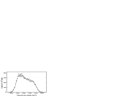
Figure 1: Peak corresponding to the 1332 keV ⁶⁰Co spectral line obtained by the p-type detector model for a neutron fluence of 10⁹ cm^-2. This model detector has the same dimensions and bias potential as the p-type detector studied by Pehl et al. [1].

As a check (since in fact the energy resolution is very sensitive to the value of $A_{h}$), the model gives the FWHM resolution of $64$ keV after a neutron fluence of 10¹⁰ cm^-2 (as shown in Fig. 2),

Figure 2: Peak corresponding to the 1332 keV ⁶⁰Co spectral line obtained by the p-type detector model for a neutron fluence of 10¹⁰ cm^-2. This model detector has the same dimensions and bias potential as the p-type detector studied by Pehl et al. [1].

to be compared with the experimental result of $70$ keV. Figures 3

Figure 3: Peak corresponding to the 1332 keV ⁶⁰Co spectral line obtained by the n-type detector model for a neutron fluence of 10⁹ cm^-2. This model detector has the same dimensions and bias potential as the n-type detector studied by Pehl et al. [1].

and 4

Figure 4: Peak corresponding to the 1332 keV ⁶⁰Co spectral line obtained by the n-type detector model for a neutron fluence of 10¹⁰ cm^-2. This model detector has the same dimensions and bias potential as the n-type detector studied by Pehl et al. [1].

show the corresponding model results for the n-type detector (model/experimental FWHM resolutions of $2.1/1.95$ keV and $2.7/2.7$ keV, respectively).

Figures 5

Figure 5: Peak corresponding to the 1332 keV ⁶⁰Co spectral line obtained by the p-type detector model for a neutron fluence of 10⁸ cm^-2. This model detector has the same dimensions and bias potential as the p-type detector studied by Pehl et al. [1].

and 6

Figure 6: Peak corresponding to the 1332 keV ⁶⁰Co spectral line obtained by the n-type detector model for a neutron fluence of 10⁸ cm^-2. This model detector has the same dimensions and bias potential as the n-type detector studied by Pehl et al. [1].

show the model results for the p-type and n-type detectors, respectively,  after a neutron fluence of 10⁸ cm^-2 (model/experimental FWHM resolutions of $1.85/2.1$ keV and $1.80/1.8$ keV, respectively). For this low fluence the model FWHM resolutions are nearly identical for the two detectors; instead the effect of hole trapping shows up in the magnitude of the shift of the peak centroid away from 1332 keV.

VI Application to the INL Micro-Detective

We exposed an ORTEC Micro-Detective (p-type) detector to a neutron fluence (from a ²⁵²Cf source) up to 10⁹ cm^-2. This exercise was intended to determine the neutron fluence at which the energy resolution of the Micro-Detective was too degraded to allow its use in place of our GMX (n-type) detector. Figure 7

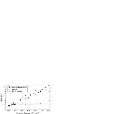
Figure 7: Measured FWHM resolution of the 1332 keV ⁶⁰Co peak obtained by the Micro-Detective and GMX detectors after various neutron fluences (where two values are shown for the same fluence, the higher/lower value was measured before/after a thermal cycle). The calculated values obtained by the Micro-Detective model are indicated by the open circles.

shows values of the FWHM resolution of the 1332 keV ⁶⁰Co peak obtained by the Micro-Detective and GMX detectors at various fluences (where two values are provided for the same fluence, the higher/lower value was measured before/after a thermal cycle). These results provide an opportunity to test the phenomenological model.

The input to the Micro-Detective model is the following: inner radius $R_{0}=4.5$ mm; outer radius $R_{1}=25$ mm; crystal length $L=30$ mm; bias potential $\phi\left(R_{1}\right)=3.0$ kV. As the dopant density is not provided, the typical value $\rho_{\text{A}}=10^{10}$ cm^-3 is used. The calculated values of the FWHM resolution, indicated by the open circles in Fig. 7, compare well with the trend of measured values. Note that the energy resolution of the Micro-Detective after a neutron fluence of 10⁹ cm^-2 is better than that of the p-type detector studied by Pehl et al. ($5.4$ keV versus $6$ keV) despite its significantly larger size (diameter $50$ mm versus $42$ mm), due to its larger bias potential ($3$ kV versus $1.6$ kV) which, by producing a stronger electric field across the crystal, reduces the hole trap cross-section.

The input to the GMX (n-type) detector model is the following: inner radius $R_{0}=5.6$ mm; outer radius $R_{1}=31.4$ mm; crystal length $L=70.3$ mm; bias potential $\phi\left(R_{0}\right)=5.0$ kV. As the dopant density is not provided, the typical value $\rho_{\text{D}}=10^{10}$ cm^-3 is used. The calculated FWHM resolutions of the 1332 keV peak at neutron fluences of 10⁸ cm^-2 and 10⁹ cm^-2 are $1.7$ keV and $2.0$ keV, respectively, in good agreement with the measured values in Fig. 7.

VII Concluding remarks

The main attributes of this model of neutron-damaged coaxial HPGe detectors are (i) the use of induced charge at the electrodes to determine the contribution of an electron-hole pair to the measured gamma-ray energy, and (ii) the use of stochastic methods to simulate what are, in fact, stochastic processes. The data of R. H. Pehl et al. [1] provided a value for the dimensionless parameter $A_{h}$, related to the probability for immediate trapping of a mobile hole, needed to complete the phenomenological model. As the model is, for the most part, one-dimensional, it is easy to implement in a computer code. However, by ignoring the detector “cap” (where the applied electric field is not purely radial), this model is not well suited for application to low-energy gamma-rays which may be substantially stopped in that volume.

Some observations: (i) The n-type detectors maintain good energy resolution to neutron fluences of at least 10⁹ cm^-2. The noticeable effect of neutron damage is to shift the peak centroid to a lower energy. (ii) The peak shapes after a high neutron fluence of 10¹⁰ cm^-2 are very different for p-type and n-type detectors. This is due not only to more hole trapping in a p-type detector, but also to the fact that an electron-hole pair with a trapped hole near the outer contact induces a smaller charge $\left|Q\right|$ at the two electrodes of a p-type detector than at the electrodes of a same-sized n-type detector (see section II for a more precise discussion of this effect). Thus those gamma-rays that interact closer to the outer contact (which is to say, most of the gamma-rays) are more likely to register as “counts” at the low/high end of the energy spectrum in the case of p-type/n-type coaxial detectors.

References

- [1] R. H. Pehl, N. W. Madden, J. H. Elliott, T. W. Raudorf, R. C. Trammell, and L. S. Darken, Jr., “Radiation damage resistance of reverse electrode Ge coaxial detectors,” IEEE Trans. Nucl. Sci., vol. NS-26, no. 1, pp. 321–323, Feb. 1979.
- [2] J. D. Jackson, Classical Electrodynamics. New York: Wiley, 1962.
- [3] G. F. Knoll, Radiation Detection and Measurement, 3rd ed. New York: Wiley, 2000.
- [4] G. E. P. Box and M. E. Muller, “A note on the generation of random normal deviates,” Ann. Math. Statist., vol. 29, no. 2, pp. 610–611, 1958.
- [5] L. S. Darken, Jr., R. C. Trammell, T. W. Raudorf, R. H. Pehl, and J. H. Elliott, “Mechanism for fast neutron damage of Ge(HP) detectors,” Nucl. Instrum. Methods, vol. 171, pp. 49–59, 1980.
- [6] T. W. Raudorf and R. H. Pehl, “Effect of charge carrier trapping on germanium coaxial detector line shapes,” Nucl. Instrum. Methods Phys. Res. A, vol. A255, pp. 538–551, 1987.
- [7] L. S. Darken, “Role of disordered regions in fast-neutron damage of HPGe detectors,” Nucl. Instrum. Methods Phys. Res., vol. B74, pp. 523–526, 1993.
- [8] L. S. Darken, Jr., R. C. Trammell, T. W. Raudorf, and R. H. Pehl, “Neutron damage in Ge(HP) coaxial detectors,” IEEE Trans. Nucl. Sci., vol. NS-28, no. 1, pp. 572–578, 1981.
- [9] Th. Kröll and D. Bazzacco, “Simulation and analysis of pulse shapes from highly segmented HPGe detectors for the -ray tracking array MARS,” Nucl. Instrum. Methods Phys. Res. A, vol. 463, pp. 227–249, 2001.