Star Clusters in M 31. IV. A Comparative Analysis of Absorption Line Indices in Old M 31 and Milky Way Clusters

Abstract

We present absorption line indices measured in the integrated spectra of globular clusters both from the Galaxy and from M 31. Our samples include 41 Galactic globular clusters, and more than 300 clusters in M 31. The conversion of instrumental equivalent widths into the Lick system is described, and zero-point uncertainties are provided. Comparison of line indices of old M 31 clusters and Galactic globular clusters suggests an absence of important differences in chemical composition between the two cluster systems. In particular, CN indices in the spectra of M 31 and Galactic clusters are essentially consistent with each other, in disagreement with several previous works. We reanalyze some of the previous data, and conclude that reported CN differences between M 31 and Galactic clusters were mostly due to data calibration uncertainties. Our data support the conclusion that the chemical compositions of Milky Way and M 31 globular clusters are not substantially different, and that there is no need to resort to enhanced nitrogen abundances to account for the optical spectra of M 31 globular clusters.

1 Introduction

The history of star formation and chemical enrichment of galaxies is encoded in the ages and chemical compositions of their stellar populations. In particular, powerful insights on the processes leading to the assembly of the Galactic halo are gained by studies of the chemical abundances of their constituent populations of field stars and globular clusters (GCs). It is only natural to extend such studies to the nearest giant spiral galaxy, M 31. While detailed abundances of individual stars in the Galactic halo, disk, and bulge, have been obtained and extensively analyzed in the past several decades, similar studies of comparable samples of M 31 halo stars await the advent of 20-30 m class telescopes, equipped with efficient high-resolution spectrographs. In the meantime, integrated light studies of M 31 GCs have historically provided valuable qualitative information about the chemical composition of the halo of M 31, leading to important clues on its formation history. As stellar population synthesis models and instruments both grow in sophistication, quantitative information on elemental abundances from integrated-light studies of M 31 GCs is also becoming available (e.g., Colucci et al., 2009; Caldwell et al., 2011).

The history of this field has been punctuated by heroic observational efforts, based on optical spectra painstakingly collected with, according to today’s standards, relatively small telescopes, rather inefficient spectrographs, and low-quantum efficiency (and often difficult to calibrate) detectors (e.g., Burstein et al., 1984; Brodie & Huchra, 1990). The main results emerging from these efforts are: 1) M 31 GCs are on average slightly more metal rich than their Galactic counterparts, while spanning roughly the same range of metallicities (Brodie & Huchra, 1991); 2) M 31 GCs are $\alpha$-enhanced, just like those in the MW (e.g., Puzia et al., 2005); 3) M 31 GCs are CN-enhanced compared to MW GCs (Burstein et al., 1984; Brodie & Huchra, 1990; Beasley et al., 2004; Puzia et al., 2005). In particular, Burstein et al. (1984) found that the CN band at $\lambda$ 4170 ${\rm\AA}$ is stronger by $\sim$ 0.05 mag in the spectra of moderately metal-poor M31 GCs than in those of their MW counterparts of same metallicity; and 4) M 31 GCs are possibly younger/older than those in the MW. Burstein et al. (1984) found that $H\beta$ is stronger in the spectra of M 31 GCs than in those of their MW counterparts by about 0.5 ${\rm\AA}$, indicating a younger age or differences in horizontal branch morphology. The latter two results are contradicted by the findings presented in this paper. While Caldwell et al. (2011) discuss the Balmer line strengths in the spectra of the two GC systems, comparing their ages, CN is the main focus of this paper.

Those significant conclusions may teach us about important aspects of the formation of the two galaxies. For instance, the comparable mean metallicities may be indicative of similar overall chemical enrichment, suggesting that the early star formation efficiency has been similar in the two systems—or perhaps in the sub-components that eventually assembled to form them. The similar $\alpha$-enhancement, assessed by measurements of Mg and Fe-sensitive absorption lines, suggests that either the time scale for star formation, the IMF, or a combination thereof, were similar in both galaxies. The difference in CN strength, which has been ascribed to a difference in nitrogen abundance, is difficult to interpret, owing mostly to uncertainties in the models for the nucleosynthesis of that element. The issue is further complicated by the fact that CNO elements are seen to present strong star-to-star variations in Galactic GCs (e.g., Gratton et al., 2004, and references therein), which may be associated with the presence of multiple stellar populations in those GCs (Conroy & Spergel, 2010; Piotto, 2009; Martell & Smith, 2009; Cannon et al., 1998, and references therein), and by inference, in their M 31 counterparts. Regardless, any scenario for the formation of the MW and M 31 haloes, and their GC systems, will be challenged by the large nitrogen abundance differences between systems that look otherwise very similar.

This is the fourth of a series of papers dedicated to analyzing the kinematics and chemistry of a large sample of M 31 GCs, based on high-quality integrated spectra for several hundred M 31 clusters, obtained with MMT/Hectospec. In Paper I (Caldwell et al., 2009) we characterized the population of young ($\mathrel{\hbox{\raise 2.15277pt\hbox{$<$}\hbox to0.0pt{\hss\lower 2.15277pt\hbox{$\sim$}}}}$ 2 Gyr) M 31 clusters in terms of their ages, metallicities, masses, and kinematics. In Paper II (Caldwell et al., 2011), the ages and metallicities of M 31 old GCs were studied. In particular, we found no differences between the ages of the two old GC systems, in disagreement with previous claims. Moreover, we found that the M 31 GC system does not have a bimodal metallicity distribution, in agreement with recent findings (Yoon et al., 2006). In Paper III (Morrison et al., 2010), we suggest that the old bulge GCs in M 31 are characterized by a bar-like kinematics.

In this paper, we present absorption line indices measured in integrated spectra of a large sample of M 31 and MW GCs. The data for M 31 GCs come from spectra described by Caldwell et al. (2009), and those for MW GCs are based on the integrated GC spectra from Schiavon et al. (2005). While the focus of this paper is on the comparison of CN strengths between the two GC systems, Schiavon et al. (2011) will present an analysis of abundance ratios, based on application of stellar population synthesis models to these index measurements. This paper is organized as follows: in Section 2, the measurement of Lick absorption line indices is described, and a comparison between CN indices in M 31 and MW GCs is presented in Section 3. Our conclusions are summarized in Section 4.

2 Data

A detailed description of our data, including sample selection, observation and reduction procedures, is presented in Schiavon et al. (2005) and Caldwell et al. (2009) for the MW and M 31 GCs, respectively. Various aspects that are relevant to this work are summarized below.

The M 31 GC spectra were obtained using the multi-fiber spectrograph Hectospec (Fabricant et al., 2005), attached to the 6.5 m Multiple Mirror Telescope (MMT). The projected diameter of a Hectospec fiber on the sky is 1$\arcsec$.5, and the spectral coverage of the resulting 1-D, wavelength-calibrated spectra, is 3650–9200 ${\rm\AA}$. Spectral dispersion, and resolution are 1.2 ${\rm\AA}$ pixel^-1 and 5${\rm\AA}$, respectively, and the median S/N of the spectra is 75 pixel^-1. The normal operating procedure with Hectospec, and other multi-fiber spectrographs, is to assign a number of fibers to blank sky areas in the focal plane, and then combine those in some fashion to allow sky subtraction of the target spectra. These methods are satisfactory for our outer M 31 fields, but not for the bulge areas where the local background is high relative to the cluster targets (and where the most metal-rich clusters reside, along with many metal-poor clusters). As described in Paper II, for the bulge clusters only sky spectra far from the bulge of M31 were used. A separate offset exposure for such fields, taken concurrently and about 5$\arcsec$ offset from the targets, was reduced in a similar way (so that contemporaneous sky subtraction was performed for on- and off-target exposures), and then these off-target local background spectra were subtracted from the on-target. Relative flux calibration, aimed at removing the signatures of instrumental and atmospheric transmission, was achieved using observations of flux standards.

The MW GC spectra were collected with the CTIO Blanco 4 m telescope, equipped with the Ritchey-Chrétien spectrograph, mounted at the telescope’s Cassegrain focus. Given the extended nature of Galactic GCs, observations were executed by drift scanning the targets with a 5$\arcmin$.5-long slit, over the range of $\pm$ one GC core radius, $r_{c}$, taken from Harris (1996). Additional exposures in areas surrounding the target GCs were obtained for background-subtraction purposes. One-dimensional spectra were extracted by coadding the columns contained within a $\pm\,\sim\,1\,r_{c}$ spatial window centered on the peak of each GC’s light profile. Therefore, for most GCs, the 1-D spectra sample a core radius-sized square spatial region (but see Schiavon et al., 2005, for exceptions). No significant variations in Lick index measurements were found between spectra that sample different spatial regions, for any of the 9 GCs for which such spectra were available. The spectra were wavelength-calibrated in the usual fashion. The resulting 1D wavelength-calibrated spectra cover the region between 3360 and 6430 ${\rm\AA}$, with a spectral dispersion of 1 ${\rm\AA}$ pixel^-1 and a resolution of $\sim$ 3.1 ${\rm\AA}$. Relative flux calibration was achieved in the usual fashion, using observations of spectrophotometric standards.

2.1 Absorption line indices

Even though the two sets of GC spectra were obtained with different instruments, and following rather different observational procedures, the measurement of line indices in the 1D spectra and their conversion from instrumental to standard system follows the same well established recipes that are only briefly described in this Section. All line indices discussed in this paper were measured with the lick_ew code, which is part of the EZ_Ages package (Graves & Schiavon, 2008). Cluster spectra were first smoothed from their original resolution to the resolution of the Lick index, system, given in Table 1 of Schiavon (2007) for each of the indices. The original resolution was 5${\rm\AA}$ in the case of the M 31 GCs, and that given in equation (1) of Schiavon et al. (2005). Instrumental index measurements are based on the definitions provided by Worthey et al. (1994) and Worthey & Ottaviani (1997). Conversion between instrumental and standard Lick indices was achieved in the usual fashion, through comparison with measurements taken in spectra of standard stars. Observation of Lick standards were obtained using the same instrumental setup used for GC observations, and the spectra reduced following the same procedures as adopted for GC spectra. Likewise, the spectra of Lick standards were smoothed to the Lick resolution, and instrumental indices measured adopting the same definitions as above. For the M 31 Hectospec data, the six standards were observed through single fibers, though each star was observed through a different fiber. No significant star-to-star variation is seen in the residuals shown in Figures 3 and 4, so we conclude that different fiber-to-fiber throughput variations contribute negligible uncertainties to our index measurements.

We note that the Tololo spectra are affected by a bad CCD column that runs across the spectra at a wavelength placed within the passband of the Lick CN indices. We measured the effect of that bad column on our index measurements and found them to be affected at the $\sim$ 0.015 mag level in the worst cases. Moreover, the effect varies in sign and intensity from GC to GC , and thus should not introduce any significant systematic effect in our measurements.

An important aspect of our conversion to the Lick system is the adoption of standard index values from Schiavon (2007), rather than those of Worthey et al. (1994). We proceeded this way because of the higher accuracy of the Schiavon (2007) indices. Because they are based on flux-calibrated CCD spectra, they are free from the uncertainties associated with difficulties in calibrating data obtained with the Lick Image Dissector Scanner, upon which the Worthey et al. (1994) indices are based. For more details, see discussion in Schiavon (2007), and particularly Figures 1 and 2 of that paper.

Figure 1: Calibration of instrumental pseudo-equivalent widths into the Lick system for the Tololo integrated spectra of Galactic GCs from Schiavon et al. (2005), using observations of Lick standards. Zero points were calculated by averaging the residuals for all indices, excluding very strong deviants. Standard Lick indices come from Schiavon (2007). Residuals are plotted as a function of instrumental index strength. Formal error bars based on photon noise, readout noise, and sky-subtraction errors are smaller than the symbol sizes and are not plotted. The few standard star observations yield somewhat uncertain zero points for some indices. See discussion in the text.

Figure 2: Figure 1 continued. Note that, except for a single very deviant measurement, residuals for CN indices are very small—in fact, much smaller than the $\sim$ 0.05 mag CN differences measured by Burstein et al. (1984) between MW and M 31 GCs. The very deviant point is due to star HD 78418, which is a spectroscopic binary. It is not clear why it is not very deviant in other indices as well. Comparison of the Tololo spectrum for this star with that from Jones (1999) suggests that there may be problems with flux calibration of the former, in the region of the CN indices.

Instrumental and standard Lick indices are compared in Figures 1 and 2 for the Tololo data, and in Figures  3 and 4 for the Hectospec data, where residuals are plotted as a function of index strength. Error bars were calculated based on propagation of photon noise, readout noise, and sky-subtraction errors into index measurements, following Cardiel et al. (1998). In the case of the Tololo data, they are smaller than the symbol sizes, and are thus not plotted. The IDs of the standard stars observed, as well as the instrumental measurements are provided in Tables 4 through 7. The standard values were taken from Schiavon (2007), for the indices modeled in that paper. The residuals are in general small, and so are the zero point corrections for all indices in both sets of observations, which is a result of the data being based on flux calibrated, high-S/N spectra, as discussed by Schiavon (2007). We note that, due mostly to unfavorable weather, we unfortunately were unable to collect data for a large number of Lick standards, particularly during the observing run in Cerro Tololo, where the Galactic GCs were observed. Therefore, as seen in those Figures, the conversion to the standard Lick system is sometimes based on a handful of data points, in most cases spanning an insufficient range of index strengths, resulting in somewhat uncertain, though small, zero point corrections. Most importantly, for the purposes of this paper, we note that the residuals of the CN indices in both data sets are very small—indeed, much smaller than the 0.05 mag CN difference found by Burstein et al. (1984) between the M 31 and MW GC systems.

For some indices, the data suggest the presence of a correlation of the residuals with index strength. That is the case of $C_{2}4668$ for the M 31 sample, and $H\delta_{A}$, $H\gamma_{A}$, $H\gamma_{F}$, and Fe4383, in the case of the MW sample. Despite the evidence for such trends, we adopt single zero-point conversions for such indices, because the range spanned by the residual variations is relatively small. For instance, according to the Schiavon (2007) models, the systematics introduced in [C/Fe] determinations by adopting a constant zero-point conversion to $C_{2}4668$ is smaller than $\sim$ 0.1 dex. By the same token, uncertainties in [Fe/H] due to zero point uncertainties in Fe4383 are smaller than 0.1 dex, and those in the Balmer lines translate into a mere $\sim$ 1 Gyr uncertainty in age, for old systems.

The final zero points are thus estimated as the mean residual, excluding strongly deviant points. The paucity of data points makes it difficult to estimate the zero point uncertainties, and to be as fair as possible, we define these as 1/2 of the dynamic range of the residuals, or:

$$\Delta Zero\,\,Point={Max(Residual)-Min(Residual)\over 2},$$ (1)

where strongly deviant points were removed from the statistics. This may be a fair representation of the uncertainties in indices that present a large scatter of the residuals (e.g., G4300) or showing an apparent trend of residuals with index strength ($H\delta_{A}$, $H\gamma_{A}$, $H\gamma_{F}$, and Fe4383), but it possibly underestimates the uncertainties for indices where little variation of the residuals is seen. However, the latter is presumably due to the indices being robust to instrumental effects, as is probably the case of $H\beta$ and redder indices—see discussion and plots in Schiavon et al. (2004a) and Schiavon (2007). The final zero point conversions to the Lick system from Schiavon (2007) and associated uncertainties are provided in Tables 1 and  2.

Finally, we decided to include, for completeness, indices that were not modeled by Schiavon (2007) , and for those they come from unpublished measurements taken on the spectra of the Indo-US library (Valdes et al., 2004), convolved to the Lick/IDS resolution (see details in Schiavon, 2007) . Conversion of the instrumental indices into the Indo-US system is provided in Tables 12 and 13 for MW and M 31 GCs, respectively. Conversion between Indo-US values and the standard Lick/IDS system of Worthey et al. (1994), based on $\sim$ 100 stars in common between the two spectral libraries, is provided in Table 14.

Figure 3: Calibration of instrumental pseudo-equivalent widths into the Lick system for the Hectospec integrated spectra of M 31 GCs, using observations of Lick standards. Zero points were calculated by averaging the residuals for all indices, excluding very strong deviants. Standard Lick indices come from Schiavon (2007). Residuals are plotted as a function of instrumental index strength. For all indices, the zero point shifts are relatively small, and fairly well determined.

Figure 4: Figure 3 continued. Note that, as in the case of the MW GCs, (Figure 2) the CN residuals are much smaller than the 0.05 mag difference between M 31 and MW GCs, found by Burstein et al. (1984).

3 MW vs M 31 globular clusters in index-index space

The two systems of GCs are compared in index-index space in Figures 5-7. We plot all indices against $\langle$Fe$\rangle$, which is the average of the two Lick indices Fe5270 and Fe5335. Schiavon (2007) showed that this combination of indices is a good indicator of [Fe/H], being only weakly sensitive to variations of other elemental abundances, and being only mildly sensitive to age and horizontal branch (HB) morphology. A relation between $\langle$Fe$\rangle$ and [Fe/H] was derived by Caldwell et al. (2011), on the basis of 31 Galactic GCs with [Fe/H] determinations from abundance analysis of high resolution spectra of individual GC member stars by Carretta et al. (2009), Kraft & Ivans (2003), and Carretta & Gratton (1997). Iron abundances in the two latter papers were converted to the Carretta et al. (2009) scale using the transformations provided in their Appendix. That relation is used to plot an approximate [Fe/H] scale on the top of the upper panels in Figures 5-7. Due to non-linearities in the $\langle$Fe$\rangle$–[Fe/H] relation, the [Fe/H] scale in those plots is only approximate, but is useful to guide the eye. For clarity and accuracy, M 31 GCs for which the error in $\langle$Fe$\rangle$ is greater than 0.15 ${\rm\AA}$ are excluded from the plots. This removes all young clusters from the M 31 sample, because the S/N of the spectra for these lower-mass, fainter clusters, is indeed on average lower than that of their older, more massive counterparts. Most importantly, the absence of young and intermediate-age GCs in the M 31 sample means that age effects are, to first order, negligible in metal-index vs. metal-index plots in Figures 5-7—though they may be detectable in plots involving Balmer lines. In this way, we can perform a reliable model-free assessment of differences (or lack thereof) between the old M 31 and MW GCs in metallicity and abundance-ratio spaces. Two sets of error bars are shown for each GC system in the upper/lower left corner of each panel. The upper set of error bars represents the average uncertainty in individual index measurements, as estimated by lick_ew, using the prescription from Cardiel et al. (1998). The lower set of error bars represents the zero point uncertainties determined as described in Section 2.1.

Before moving to the main focus of this paper, which is a comparison of the strengths of CN indices in M 31 and MW GCs, we briefly mention a few interesting features of Figures 5-7. The first obvious feature is the systematic difference between the two GC samples in C${}_{2}4668$, where M 31 GCs are systematically stronger by $\sim$ 0.5 ${\rm\AA}$. We note that the calibration of this index into the Lick system is relatively uncertain, as indicated by the error bars on the top left panel of Figure 7, whose size is in fact comparable to the shift between the two samples. If taken at face value, this discrepancy could indicate a higher [C/Fe] in M 31 GCs than in their MW counterparts. However, the data for the other carbon-sensitive index in this study, G4300, are not consistent with that interpretation (Figure 6). For [Fe/H] $\mathrel{\hbox{\raise 2.15277pt\hbox{$<$}\hbox to0.0pt{\hss\lower 2.15277pt\hbox{$\sim$}}}}$ –1.2, the two samples seem to have identical G4300 values, and for higher [Fe/H] MW GCs actually have stronger G4300 than their M 31 counterparts. The latter is most likely not associated with a difference in [C/Fe], but rather with differences in age indicators between metal-rich MW and M 31 GCs, which are not completely understood (see discussion in Section 3.2). We therefore conclude that the differences seen in C${}_{2}4668$ are probably a spurious effect due to uncertainties in the calibration of that index. This topic will be revisited in a forthcoming paper, where abundance ratios for both samples will be determined and analyzed.

We finally point out that systematic differences between M 31 and MW GCs with [Fe/H] $\mathrel{\hbox{\raise 2.15277pt\hbox{$>$}\hbox to0.0pt{\hss\lower 2.15277pt\hbox{$\sim$}}}}$ –1.2 can be seen in Figures 5 and 6 in the strengths of their $H\delta$ and $H\gamma$ indices. Interestingly, no such systematics are seen in $H\beta$. A comparative analysis of Balmer line strengths in the two GC samples is the topic of another forthcoming paper.

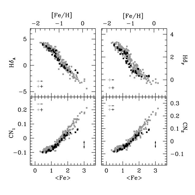
Figure 5: Lick indices for M 31 (gray) and MW (black) GCs. Only GCs for which the error in $\langle$Fe$\rangle$ is smaller than 0.15 ${\rm\AA}$ are plotted. Two sets of error bars are shown for each GC system in the upper/lower left corner of each panel. The upper set represents the average uncertainty in individual index measurements, as estimated by lick_ew, using the prescription from Cardiel et al. (1998). The lower set represents the zero point uncertainties determined as described in Section 2.1. The average $\langle$Fe$\rangle$ index is a good indicator of [Fe/H], and a $\langle$Fe$\rangle$–[Fe/H] relation derived by Caldwell et al. (2011) is used to establish the [Fe/H] scale at the top of the upper panels. That relation is strongly non-linear for [Fe/H]$\mathrel{\hbox{\raise 2.15277pt\hbox{$<$}\hbox to0.0pt{\hss\lower 2.15277pt\hbox{$\sim$}}}}-1.5$ and [Fe/H]$\mathrel{\hbox{\raise 2.15277pt\hbox{$>$}\hbox to0.0pt{\hss\lower 2.15277pt\hbox{$\sim$}}}}0.0$. Within the uncertainties, there is no systematic difference between the two GC systems in either $H\delta$ or CN indices—certainly nothing as high as 0.05 mag, as found by Burstein et al. (1984). The arrows in the lower right of the bottom panels indicate the size of the effect found by Burstein et al. (1984). The exceptions are the two most metal-rich MW GCs, NGC 6528 and 6553 (where the former is represented by the two highest $\langle$Fe$\rangle$ data points—see text). These GCs are systematically weaker in CN and stronger in H$\delta$, than M 31 GCs of the same [Fe/H]—see discussion in text.

Figure 6: Same as Figure 5 for another set of line indices. Again, no significant differences between the two GC systems in index-index space is found, again, with the exception of NGC 6528 and 6553, which are too strong in $H\gamma$ and too weak in G4300, compared to M 31 GCs of the same [Fe/H]. A few MW clusters seem to deviate from the trends established by the remaining Galactic objects—see discussion in text.

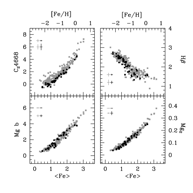
Figure 7: Same as Figure 5 for another set of line indices. No significant difference between the two GC systems is detected in $H\beta$ or Mg indices. There is a hint that $C_{2}4668$ may be stronger in M 31 GCs than in their MW counterparts of same [Fe/H], which would be indicative of a higher carbon abundance in M 31 GCs. However, the difference is not larger than the zero-point uncertainty for this index, which is particularly large for both data sets. Unlike in the case of the bluer Lick indices, the two metal-rich MW GCs do not differ from their M 31 counterparts in any of the indices displayed here.

3.1 Fe vs CN indices

We focus on the bottom panels of Figure 5, which compare the two GC samples in $\langle$Fe$\rangle$-CN space. Note that the two CN indices displayed in this Figure behave in exactly the same way. This is because these indices measure the same spectral feature, which is a combination of $\Delta v$ = 0 and –1 vibrational bands of the CN violet electronic transition ($B_{2}\Sigma-X^{2}\Sigma$), spreading roughly between 4100 and 4220 ${\rm\AA}$ (Wallace, 1962). The only difference between the two indices is in the blue pseudocontinuum, which in the case of the $CN_{2}$ index is slightly narrower. Because our results are independent of which of the two indices is used, we throughout this paper sometimes refer to CN indices as both $CN_{1}$ and $CN_{2}$ Lick indices.

In this section, we concentrate our attention on GCs more metal-poor than [Fe/H] $\sim$ –0.4, leaving the discussion of the more metal-rich GCs for Section 3.2. The most obvious feature in these plots is the slight difference between the two GC samples in CN strength. We find an average CN difference between M 31 and MW GCs of about 0.01 mag, which is the same size as the zero-point uncertainties in both sets of measurements. This difference is also 1/5 of what was found by Burstein et al. (1984) (indicated by arrows in the lower right of the bottom panels). In other words, spectra of MW and M 31 GCs of the same $\langle$Fe$\rangle$ (same [Fe/H]) seem to have essentially the same CN strength (we discuss the deviant, high-metallicity, MW GCs below). This is in disagreement with the results of Burstein et al. (1984), Beasley et al. (2004), and Puzia et al. (2005), who measured the same indices in smaller samples of lower S/N spectra, finding evidence for a difference between the two GC systems, in that M 31 GCs have stronger CN than their MW counterparts by about 0.05 mag. Similar CN differences between MW and M 31 GCs were also suggested by Brodie & Huchra (1990), who measured the strengths of the same CN bands studied in this paper, in a sample consisting of tens of M 31 and MW GCs. Similar differences were also found by Davidge (1990), who measured the strength of CN bands in NIR spectra of four M 31 GCs. Because no difference was found between the two GC systems in a carbon-sensitive index (the G band), the above authors suggested that the CN differences were probably due to M 31 GCs having higher nitrogen abundances than their MW counterparts. Just how much higher should the [N/Fe] values be in M 31 than in MW GCs was not known, as such an estimate required models that were then unavailable. Nevertheless, that suggestion was later bolstered by measurements of the near-UV NH band at 3360${\rm\AA}$ by Ponder et al. (1998), Li & Burstein (2003), and Burstein et al. (2004). In particular, Burstein et al. (2004) found NH3360 to be stronger in M 31 than in MW GCs by over $\sim$ 2 ${\rm\AA}$ (see discussion in Section 3.1.2).

Our result is then rather surprising, in view of the relatively large body of counter-evidence summarized above, which led to the (far-reaching) conclusion that M 31 and MW GCs have different nitrogen abundances. Considering the significance of the zero point uncertainties discussed in Section 2.1, we decided to take advantage of the high S/N of our data to inspect visually the spectra of M 31 and MW GCs. That required selecting GCs with the same [Fe/H] and same combination of age and HB morphology. We proceeded as follows. We first selected four MW GCs spanning a wide range of metallicities for the comparison: NGC 2298, NGC 1851, 47 Tuc, and NGC 6528, with [Fe/H] = -1.96, -1,18, -0.76, and +0.07 (Carretta et al., 2009). Next, we looked for M 31 GCs with similar parameters. The search is illustrated in Figure 8, where data for those four GCs are overplotted on top of M 31 GC measurements in the $\langle$Fe$\rangle\times\,H\beta$ plane. Schiavon et al. (2004b) and Schiavon (2007) showed that these indices are chiefly sensitive to [Fe/H], age, and HB morphology. Therefore, selecting M 31 GCs with similar $\langle$Fe$\rangle$ and $H\beta$, one should obtain a sample with [Fe/H] and age/HB-morphology that is similar to those of the four MW GCs of choice. The boxes surrounding the latter four data points illustrate our selection of four sub-samples of GCs which are the counterparts of NGC 2298, NGC 1851, 47 Tuc, and NGC 6528 in M 31, according to that (limited) set of stellar population parameters. Clusters with low S/N spectra or unusual-looking spectral shapes (indicative of uncertain flux-calibration) were removed from the sub-samples. The IDs of the GCs selected for each metallicity bin are listed in Table 3. Intercomparison of these spectra should reveal any CN differences that may be masked by zero-point uncertainties in our Lick index measurements. Very high S/N stacked spectra of M 31 GCs within each of the four metallicity groups were generated, which are compared with those of their MW counterparts in Figure 9. The latter spectra were smoothed to match the lower resolution of the M 31 GCs spectra. In all panels, the wavelengths of the pseudocontinuum and passband windows defining the Lick $CN_{1}$ index are indicated as horizontal bars, and $CN_{1}$ measurements taken on these spectra are shown in the lower-right corner of each panel. Another bar towards shorter wavelengths indicates the approximate span of the (stronger) violet CN bands, which go from roughly 3840 to 3890 ${\rm\AA}$ (Wallace, 1962)

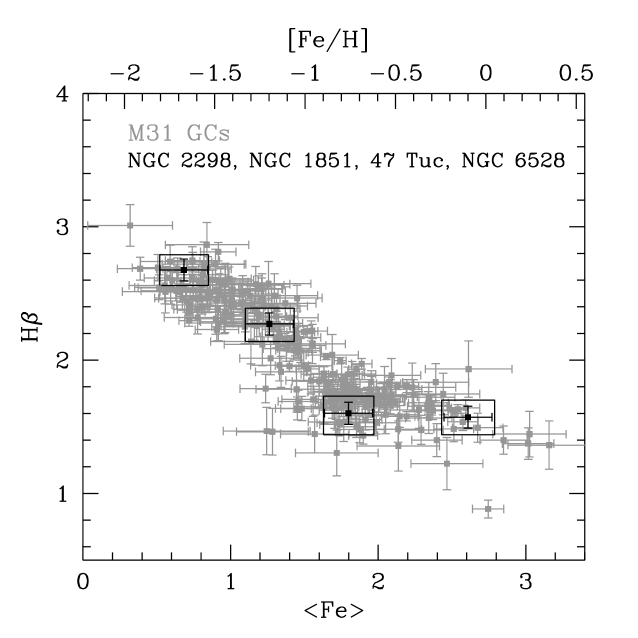
Figure 8: This figure illustrates our criteria to select MW and M 31 GCs for spectral comparison. Data in gray represent measurements in M 31 GC spectra. The black data points represent the measurements and error bars for four MW GCs, spanning a wide range of [Fe/H]. The boxes surrounding the MW GC data points represent the index bounds for the search of similar GCs in M 31. Those M 31 GCs that fall inside each search box are deemed similar to their MW counterparts in terms of [Fe/H] and a combination of age and HB morphology. The spectra of these M 31 GCs are stacked and compared with their MW counterparts, as shown in subsequent Figures.

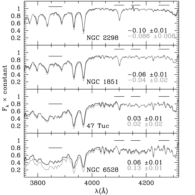
Figure 9: Comparison of MW and M 31 GCs spectra selected according to the criteria described in Figure 8. MW GCs are plotted in black, M 31 GCs in gray. Each spectrum was multiplied by a constant, so that the average flux within the red pseudocontinuum of the Lick CN index are approximately the same. MW GC spectra were smoothed in order to match the lower resolution of M 31 spectra. $CN_{1}$ indices measured in the MW spectra and the average index values for M 31 GCs are displayed at the lower right corner of each panel. Horizontal bars at upper right of each panel represent the pseudo-continuum windows and passband of the $CN_{1}$ index. The horizontal bar towards shorter wavelengths indicates the approximate span of the CN violet bands. Except for NGC 6528, there is no indication for a difference in CN-band strength between MW and M 31 GCs. See discussion in the text.

We first focus on the spectra of NGC 2298, NGC 1851, and 47 Tuc, leaving the discussion of NGC 6528 to Section 3.2. The spectra of these three clusters are remarkably similar to those of their M 31 counterparts, except for slight slope differences, which can be ascribed to uncertainties in flux calibration and reddening. There are also small differences in the strengths of Ca HK and higher order Balmer lines, which may be due to a combination of sky-subtraction uncertainties and genuine differences in the relative numbers of the hottest stars and their temperature distributions (a topic that is further discussed in a forthcoming paper). However, in confirmation of our conclusions from Figure 5, there are no differences in CN strengths between these two sets of spectra, either in the 4170 $CN_{1}$ band, or in the violet CN band. The latter is particularly important because the violet CN band is more sensitive than its blue counterpart to variations of CN concentration in stellar atmospheres, further reinforcing the notion that there are no differences in CN strengths between M 31 and MW GCs. For NGC 2298, NGC 1851, and their M 31 counterparts, the spectral shape and the strengths of the lines included in the bandpass of the $CN_{1}$ index suggest that blue CN lines are indeed very weak, if not altogether absent, from the spectrum. Therefore, we suggest that any differences between M 31 and MW spectra in this low metallicity regime cannot be ascribed to differences in CN strength (the 0.014 mag difference measured in $CN_{1}$ between NGC 2298 and its M 31 counterparts is mostly due to the blip in the spectrum of NGC 2298, which is associated with a bad CCD column, as discussed in Section 2.1). These comparisons also suggest that zero-point uncertainties in $CN_{1}$ measurements are negligible.

Having found no compelling reasons in our own data to conclude that there is any significant CN-strength difference between M 31 and MW GCs, we examine other data sets published in the literature, in an attempt to understand the contrast between our results and those from other studies. This is the topic of the next three sub-sections.

3.1.1 The Puzia et al. data

The result above is further confirmed by inspection of other data sets, such as those published by T. Puzia and collaborators. Puzia et al. (2002) obtained integrated spectra for Galactic GCs, with a resolution of 6.7 ${\rm\AA}$, using the Boller & Chivens spectrograph attached to the 1.52 m telescope at ESO/La Silla. The observational strategy followed by Puzia et al. (2002) differs from that of Schiavon et al. (2005) in two important aspects. The first concerns the sampling of the extended GC spatial distributions. While Schiavon et al. (2005) drift-scanned the target GCs within their core radii, Puzia et al. (2002) chose instead to take a number of exposures with the slit placed at different positions on the GCs. The second regards sky subtraction. Schiavon et al. (2005) scanned regions of sky around the GCs generating 1D background spectra which they subtracted from the GC extracted 1D spectra. Puzia et al. (2002) followed two different procedures. On one hand, like Schiavon et al. (2005), they subtracted 1D background spectra from their extracted cluster spectra (background “modeling”). On the other they used narrow windows at the slit ends to sample the sky background, subtracting it in the process of extracting the 1D spectrum (background “extraction”). They argue that background “modeling” yields unreliable results, because it is difficult to model the light around the clusters, mostly due to superposition of different stellar populations, and reddening variations at 1.5$\arcmin$ scales. The Puzia et al. (2005) M 31 GC data were obtained by Perrett et al. (2002) using the Wide Field Fibre Optic Spectrograph on the 4 m William Herschel Telescope at La Palma, Canary Islands. Those data resemble our own M 31 data in terms of spatial sampling, although their resolution and S/N is somewhat lower.

In Figure 10, we inter-compare data from Puzia et al. (2002) and Puzia et al. (2005) for MW and M 31 GCs, respectively. Index measurements are those in the Worthey et al. (1994) system. The mean index errors for M 31 GCs, taken from Puzia et al. (2005), are represented by error bars in each panel. The nominal measurement errors from Puzia et al. (2002) for MW GCs are comparable to symbol sizes, and are not shown. The left panels show the Lick $CN_{1}$ and $CN_{2}$ indices plotted against $\langle$Fe$\rangle$. On both panels, M 31 and MW GCs occupy approximately the same locus. There is no compelling evidence for M 31 GCs having stronger CN indices at fixed $\langle$Fe$\rangle$ (fixed [Fe/H]). The right panels show CN indices plotted against the [MgFe]’ index, which is defined as

$$[MgFe]^{\prime}=\sqrt{Mgb(0.72Fe5270+0.28Fe5335)}.$$ (2)

Again, no formal difference is found between the two GC systems in these diagrams. The MW GCs seem to occupy the lower envelope of the distribution of M 31 GCs in the [MgFe]’ vs. $CN_{2}$ plane. However, since there are no differences in the $\langle$Fe$\rangle$ vs. $CN_{2}$ plane, this mismatch is likely to be due to Mg $b$ differences between the two GC systems in the data by Puzia and collaborators, and not in their CN strengths. The latter suspicion is confirmed by Figure 11, where Mg $b$ and $\langle$Fe$\rangle$ from Puzia et al. (2002) and Puzia et al. (2005) are compared. The MW data are systematically stronger in Mg $b$ for fixed $\langle$Fe$\rangle$ than M 31 data, by about 0.5 ${\rm\AA}$. Following a suggestion by the anonymous referee, we generated plots similar to Figure 11, replacing $\langle$Fe$\rangle$ by other Fe indices, such as Fe4383, Fe4531, Fe5406, and Fe5709, and Mg $b$ by Mg₂, and the same result is obtained: MW clusters are systematically stronger than their M 31 counterparts in Mg indices at fixed Fe, which suggests that the difference is due to Mg $b$ being stronger, and not $\langle$Fe$\rangle$ being weaker, in MW clusters. We note that no such difference is found in our data between MW and M 31 (Figure 7), so we do not understand the origin of this discrepancy in the data by Puzia and collaborators. Comparing Mg $b$ for MW clusters in common between Puzia et al. (2002) and Schiavon (2007), we find that indeed the former are on average stronger by $\sim 0.13~{}{\rm\AA}$. On the other hand, comparing the Puzia et al. (2005) data for M 31 clusters with our own data for clusters in common, we find their Mg $b$ values to be on average $\sim 0.3~{}{\rm\AA}$ weaker and their $\langle$Fe$\rangle$ values to be $\sim 0.1~{}{\rm\AA}$ weaker. Incidentally, we also found the $CN_{1}$ and $CN_{2}$ values in Puzia et al. (2005) M 31 GC data to be systematically stronger than our own values by $\sim 0.02-0.03$ mag, which may also be partly responsible for their results. We note that the Perrett et al. (2002) and Puzia et al. (2005) M 31 GC data do not seem to have been flux calibrated, and moreover their line indices were not transformed to the Lick system through the comparison of observations of Lick standards with tabulated values. Therefore, we have reasons to suspect that the Puzia et al. (2005) index values may be subject to systematic effects, which may explain the discrepancies found in Figure 11.

In summary, we conclude that the data by Puzia et al. (2002) and Puzia et al. (2005) are probably consistent with no difference in CN strength between the M 31 and MW GCs.

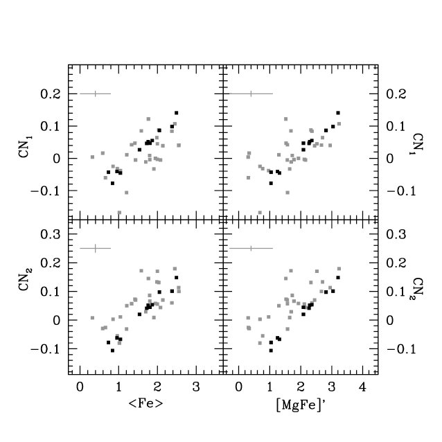
Figure 10: Data from Puzia et al. (2005) for M 31 GCs are compared with data from Puzia et al. (2002) for MW GCs. Taking error bars at face value, there is formally no difference between CN strengths in M 31 and MW GCs according to these data sets. The lower-right panel suggests a possible difference, with the M 31 GCs being stronger than MW GCs by an amount comparable to the 0.05 mag suggested by Burstein et al. (1984). We suggest that this is because of a difference in Mg $b$, rather than CN, as argued in Figure 11.

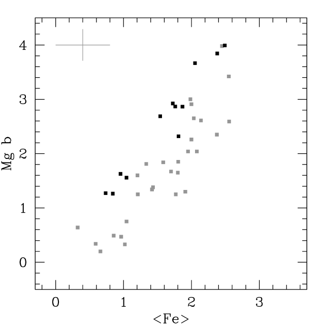
Figure 11: Data from Puzia et al. (2005) for M 31 GCs are compared with data from Puzia et al. (2002) for MW GCs. The latter have stronger Mg $b$ for given $\langle$Fe$\rangle$, suggesting that the differences between the two samples in the lower right panel of Figure 10 are in fact due to a discrepancy in Mg $b$, not in CN. We note that our data do not show any differences between M 31 and MW GCs in Mg indices, and ascribe this discrepancy in the data by Puzia and collaborators to possible calibration uncertainties.

3.1.2 The Burstein et al. (2004) data

Close inspection of other data sets also confirm our results. For instance, Burstein et al. (2004) claimed that the UV NH band at $\sim$ 3360 ${\rm\AA}$ is substantially stronger in the spectra of M 31 GCs than in their MW counterparts. Burstein et al. (2004) argue that this is further evidence for a difference in nitrogen abundance between M 31 and MW GCs—the claimed physical origin for the alleged CN differences between the two GC systems. Figure 12 shows the data from Burstein et al. (2004) for the NH 3360 and Mg₂ indices. The left panel is a reproduction of the top panel of their Figure 7, which suggests that the NH 3360 band is much stronger in M 31 GCs than in their MW counterparts. The mean indices for the bulk of the MW sample in Burstein et al. (2004) are Mg₂ $\sim$ 0.06 mag, and NH 3360 $\sim$ 3.5 ${\rm\AA}$ (excluding M 71, the GC with highest metallicity in that sample). Clusters in M 31 with comparable Mg₂ strength have NH 3360 $\sim$ 6 ${\rm\AA}$, which is almost a factor of 2 stronger than their MW counterparts.

We compared the Mg₂ measurements in Burstein et al. (2004) with our numbers for GCs in common in the two studies. From 14 M 31 GCs in common between this work and Burstein et al. (2004), we determine a mean Mg₂ difference of

$$Mg_{2}(This\,\,work)-Mg_{2}(B04)=0.052\pm 0.005\,\,mag$$ (3)

The anonymous referee pointed out to us that a systematic difference exists between the Burstein et al. (2004) Mg₂ data for M 31 GCs and those by Trager et al. (1998), which is consistent with these numbers.

For the MW sample, there are unfortunately only 3 GCs in common between the two studies: NGC 5904, 7078, and 7089, so zero point differences cannot be determined as robustly. Nevertheless, the differences between Mg₂ measurements from Burstein et al. (2004) and this work, in the same sense as above, for these three GCs, are: 0.0089, 0.0062, and 0.0038 mag, respectively. These are an order of magnitude smaller than the zero-point differences for the M 31 sample, and in fact are comparable to our zero point uncertainty from equation 1. We apply these zero point corrections to the Burstein et al. (2004) Mg₂ data, and redisplay them on the right panel of Figure 12. One can see from this Figure that most of the difference between the two samples disappears once the Burstein et al. (2004) Mg₂ indices are brought into consistency with our values. This analysis therefore suggests that most of the apparent discrepancy between NH 3360 measurements in M 31 and MW GCs is in fact due to uncertainties in the calibration of Mg₂ measurements to a common system, and not to a real difference in NH strengths.

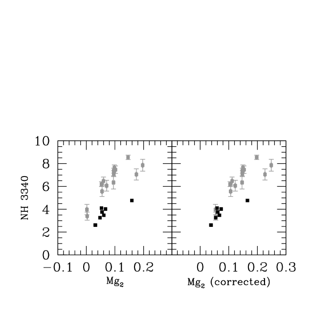
Figure 12: Left Panel: Data from Burstein et al. (2004) for M 31 (gray), and MW GCs (black). The data suggest that M 31 GCs have stronger NH bands than their MW counterparts with same Mg₂. Right Panel: Same data, but with Mg₂ indices zero-point corrected, to bring them to the same system as the data presented in this paper, using GCs in common with the two samples. Except for the most metal-rich GCs in the MW sample (M 71), MW GCs seem to have NH strengths that are consistent with those of their M 31 counterparts. This plot suggests that there may be problems with the zero-points of Mg₂ indices in Burstein et al. (2004) data, and when this effect is removed, they are in fact consistent with similar NH strengths in MW and M 31 GCs.

That there might be issues with the calibration of the Mg₂ index into the Lick system is not entirely implausible, since this index is measured on a wide baseline, being thus susceptible to uncertainties in flux calibration. However, a $\sim$ 0.05 mag difference seems too large to be explained by spectrophotometric errors alone. Burstein et al. (2004) indices for M 31 and MW GCs were measured on flux-calibrated spectra obtained, respectively, with the Blue Channel spectrograph, at MMT, and the Boller & Chivens spectrograph on the Cassegrain focus of the Bok telescope. Instrumental magnitudes were converted to the Lick system using observations of standard stars, in the usual way. We do not find any obvious way in which the calibration of Mg₂ measurements in Burstein et al. (2004) data may be faulty. By the same token, the calibration of our own measurements for that index into the Lick system seems to be quite robust (upper panel of Figure 4). However, an issue indeed seems to be present with the Burstein et al. (2004) Mg₂ indices for M 31 GCs. This is further illustrated by Figure 13, where Mg₂ measurements from different sources for M 31 and MW GCs are plotted against [Fe/H]. Iron abundances for the M 31 GCs were obtained by Caldwell et al. (2011) as described in Section 3. For MW GCs, [Fe/H] comes from Carretta et al. (2009), whereas Mg₂ comes from different sources: MW GCs from this work (gray error bars), MW GCs from Burstein et al. (2004) (solid squares), M 31 GCs from Burstein et al. (2004) (solid triangles), and M 31 GCs from Puzia et al. (2005) (open stars). Clusters in M 31 and the MW are expected to occupy the same locus in this diagram, provided they have similar [Mg/Fe], which is the case, as demonstrated by Colucci et al. (2009), Schiavon et al. (2011), and Figure 6. As can be seen, the data by Puzia et al. (2005) are in good agreement with our MW data, and so are the MW data by Burstein et al. (2004). However, the M 31 data by Burstein et al. (2004) clearly depart from the overall trend, towards lower Mg₂, suggesting a zero point offset of about 0.05 mag in that index.

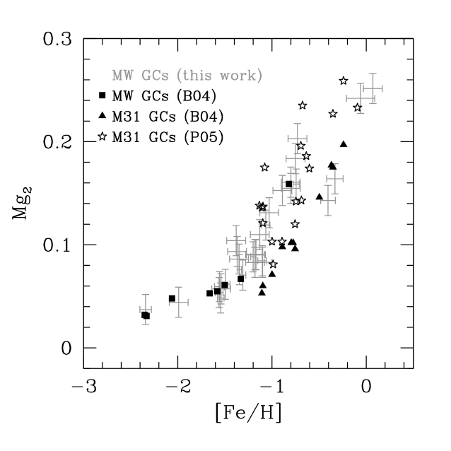
Figure 13: Run of Mg₂ with [Fe/H] for MW and M 31 GCs. Mg₂ comes from different sources: Gray error bars: MW GCs from Schiavon et al. (2005); solid squares: MW GCs from Burstein et al. (2004); solid triangles: Burstein et al. (2004) data for M 31 GCs; open stars Puzia et al. (2005) data for M 31 GCs. Iron abundances for M 31 GCs were determined using the Schiavon (2007) models, by Caldwell et al. (2011), and do not rely on Mg₂ measurements. For MW GCs, [Fe/H] comes from Carretta et al. (2009). All the data for both M 31 and MW GCs occupy the same locus in this plane, except for the Burstein et al. (2004) data for M 31 clusters, suggesting that there indeed is a zero-point offset for this index in Burstein et al. (2004) data.

We conclude that the NH 3360 feature has similar strength in the spectra of M 31 and MW GCs of the same metallicity. We suggest that the assertion that it may be stronger in the spectra of M 31 GCs derived from a zero point offset in Mg₂ measurements in Burstein et al. (2004). M 31 and MW GCs of different metallicities were compared in the NH vs Mg₂ plane, which led to a perception that NH features seemed (artificially) stronger in M 31 than in MW GCs. Therefore, we conclude that the data do not require M 31 GCs to have enhanced N abundances, relative to their MW counterparts of same metallicity. In retrospect, this is not surprising. Looking carefully at the original data by Burstein et al. (1984) and Brodie & Huchra (1990), one notices that the bulk of the difference between the two samples happens in the low metallicity regime. For instance, looking at Figure 5l in Burstein et al. (1984), one finds that CN differences between M 31 and MW GCs happen for GCs with Mg${}_{2}\,\mathrel{\hbox{\raise 2.15277pt\hbox{$<$}\hbox to0.0pt{\hss\lower 2.15277pt\hbox{$\sim$}}}}\,0.1$, which, according to Figure 13, corresponds to [Fe/H] $\mathrel{\hbox{\raise 2.15277pt\hbox{$<$}\hbox to0.0pt{\hss\lower 2.15277pt\hbox{$\sim$}}}}$ –1.0—the same actually applies to the Brodie & Huchra (1990) data. Recall that we concluded, in our discussion of GC blue spectra from Section 3.1 (Figure 9), that CN 4170 is hardly present in GCs with such low metallicities, suggesting that the measured differences may be associated with uncertainties in the calibration of the CN and/or Mg indices.

3.1.3 The Beasley et al. data

We also examine the claim by Beasley et al. (2004) that CN is enhanced in M 31 GCs. Beasley et al. (2004) obtained high S/N integrated spectra of $\sim$ 30 M 31 GCs with the LRIS spectrograph connected to the Keck I telescope. The spectra were reduced following standard procedures, and the authors report flux calibration uncertainties of the order of 10%. Indices were measured in M 31 GC spectra and converted to the Lick system using observations of standard stars. These indices were compared with measurements taken on Galactic spectra by Cohen et al. (1998) and Puzia et al. (2002).

Figure 3 of Beasley et al. (2004) shows very clearly that there are no differences in the Lick CN₂ index between M 31 and MW GCs of same metallicity. However, Beasley et al. (2004) claim that instead there are differences in the CNB index, defined by Brodie & Hanes (1986), which measures the strength of the violet CN 3883 ${\rm\AA}$ feature. Figure 4 of Beasley et al. (2004) suggests that this index is stronger in M 31 GCs than in their MW counterparts by as much as 0.1 mag. Because this result is in disagreement with their own measurements of the Lick CN indices, Beasley et al. (2004) provide a comparison between two well observed spectra from the M 31 and the Galaxy: those of 255-280 and NGC 6441, respectively. This comparison, in the form of a ratio spectrum, is shown in their Figure 5, where residuals are seen at the positions of the Lick CN₂ and CNB indices, as well as the Ca II H and K lines. The latter residual is particularly strong. However, closer inspection of that figure shows that the “feature” in the ratio spectrum below $\sim$ 4000 ${\rm\AA}$ is very broad with FWHM $\sim$ 200 ${\rm\AA}$, whereas the CN violet feature is certainly not broader than 100 ${\rm\AA}$ (see Figure 9). This suggests that the difference may be instead due to some systematic flux calibration effect, rather than to a real difference in CN strength.

This is further verified in Figure 14, where the same ratio spectrum obtained with our own data for NGC 6441 and 225-280 (gray lines) is compared with the ratio between the spectra of NGC 6441 and the average spectrum of M 31 GCs with similar [Fe/H] and age/HB-morphology as NGC 6441 (black line). Focusing first on the gray line, we note that our version of the ratio between the spectra of NGC 6441 and 225-280 is very different from that shown in Figure 5 of Beasley et al. (2004). The residual at the position of the CN violet band has a completely different shape than that shown in Figure 5 of Beasley et al. (2004). While in our case the residual keeps a strong resemblance to the shape of the CN violet band, in Beasley et al. (2004) it is indeed much broader and stronger, suggesting that it is very likely due to flux calibration and or sky-subtraction uncertainties. Such uncertainties are not unusual at the blue end of the spectrum, which is often characterized by low S/N, due to a combination of low detector quantum efficiency, high atmospheric extinction and sky background, and the overall redness of the GCs. Nevertheless, the fact remains that our ratio spectrum does show a strong residual at the position of both the violet and the Lick CN bands. This is explained, however, by the fact that 225-280 is more metal-rich than NGC 6441, as indicated by the presence of strong residuals for several other metal lines, such as Ca4227, G4300, Fe4383 (indicated in Figure 14), Mg $b$, Fe5270, Fe5335 (not shown) and many others. Running data for both GCs through EZ_Ages (Graves & Schiavon, 2008), we find that [Fe/H] is approximately 0.2 dex higher in 225-280 than in NGC 6441. Therefore, it would not be at all unexpected that CN bands are stronger in 225-280, even if the GC has the same abundance pattern than that of NGC 6441. When the spectrum of NGC 6441 is divided by the average spectrum of GCs that are more similar in metallicity, all residuals are considerably smaller (black line). Comparison of the spectrum of NGC 6441 to those of some M 31 GCs with similar metallicity, such as 073-134, 106-168, and 383-318, shows essentially no residuals at the positions of CN bands. We note that the average spectrum used to obtain the ratio displayed in Figure 14 includes GCs selected according to the following criteria: $H\delta_{F}=H\delta_{F\,6441}\pm 0.3{\rm\AA}$ and $\langle{\rm Fe}\rangle,=\,\langle{\rm Fe}\rangle_{6441}\pm 0.2{\rm\AA}$. The reason for using $H\delta_{F}$ instead of $H\beta$ has to do with the presence of blue horizontal-branch stars in NGC 6441. This is going to be discussed in a lot more detail in a forthcoming paper.

As a final note, we call attention to the fact that there is a very strong residual in the CaII H and K lines at 3968 and 3933 ${\rm\AA}$, respectively. We currently do not understand the origin of this substantial difference between M 31 and MW GCs. If real, this issue merits further scrutiny. See discussion in Section 3.2.

In summary, we conclude that the data by Beasley et al. (2004) are also consistent with our finding, that there is no substantial difference between Galactic and M 31 GCs in terms of their CN strengths. The conclusion by Beasley et al. (2004) that the violet CN band indicates such differences is possibly the by-product of a mismatch between the metallicities of the GCs analyzed, combined with flux calibration uncertainties in the violet part of the spectrum, where S/N is lower and the sensitivity function as a function of wavelength in CCD-based optical spectrographs is steep.

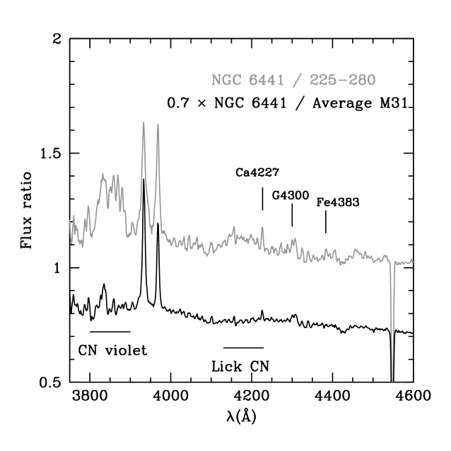
Figure 14: Ratio between the spectra of NGC 6441 and M 31 GCs. The gray line shows the ratio between NGC 6441 and 225-280 (Beasley et al., 2004) and the black line that between NGC 6441 and the average spectrum of M 31 GCs with same metallicity and age/HB-morphology. The gray line shows that, contrary to the suggestion by Beasley et al. (2004), 225-280 is more metal-rich, rather than CN-enhanced relative to NGC 6441. Residuals due to CN bands essentially vanish when NGC 6441 is compared with GCs of same metallicity. See text

3.2 The case of NGC 6528 and NGC 6553

Based on the previous section, one concludes that there is no significant difference in CN strength between M 31 and MW GCs with $[Fe/H]\mathrel{\hbox{\raise 2.15277pt\hbox{$<$}\hbox to0.0pt{\hss\lower 2.15277pt\hbox{$\sim$}}}}-0.4$. The same cannot be said about more metal-rich GCs, since the three data points at the high-metallicity end of the MW GC sample have substantially lower CN indices than their M 31 counterparts at the same [Fe/H]. Moreover, these three high-[Fe/H] MW points seem to depart significantly from the $\langle$Fe$\rangle$–$CN_{1}$ and $\langle$Fe$\rangle$–$CN_{2}$ trends established by the MW GCs alone, by being displaced towards low CN values. The two highest $\langle$Fe$\rangle$ points are from two spectra of NGC 6528, obtained with different spatial extraction windows during data reduction (see Schiavon et al., 2005, for details), whereas the third point comes from the spectrum of NGC 6553 (a third metal-rich GC, NGC 5927, also seems to be marginally too weak in CN). Visual confirmation of this result is offered at the bottom panel of Figure 9 where the spectrum of NGC 6528 is compared to the average spectrum of its M 31 counterparts. CN bands seem to be stronger in the average M 31 GC spectrum than in that of NGC 6528. Moreover, all features bluer than 4000 ${\rm\AA}$, and particularly the CaII H and K lines, are weaker in NGC 6528.

The GCs NGC 6553 and 6528 are also the two most metal-rich in the Puzia et al. (2002) sample, and no such difference between these GCs and their M 31 counterparts is seen in their data (Figure 10). According to Puzia et al. (2002), the $CN_{1}$ index is stronger in the spectra of NGC 6528 and 6553 by 0.035 and 0.096 mag than in Schiavon et al. (2005). One therefore is left wondering whether these differences may be due to different treatments of sky subtraction and spatial sampling adopted by Puzia et al. (2002) and Schiavon et al. (2005). Let us recall that NGC 6528 and 6553 are located towards the Galactic bulge, in a region of the sky that is affected by strong background and foreground contamination, rendering the task of sky subtraction rather tricky and prone to large uncertainties. Moreover, these GCs, and NGC 6553 in particular, are fairly sparse, making a fair representation of all stellar types contributing relevantly to the integrated light rather difficult, particularly for giant stars (regardless of the strengths of CN bands in their spectra).

A ratio between the spectra of NGC 6528 and its M 31 counterparts from Table 3, displayed in Figure 15 (gray line), shows the apparent signature of excess absorption in the regions of the violet and Lick CN bands in spectra of M 31 GCs. In order to check whether sky subtraction errors can be responsible for the differences found, we generated a new NGC 6528 spectrum, where the sky subtraction was changed by multiplying the sky level by 20. The ratio between NGC 6528 and that over-sky-subtracted spectrum is shown as a solid line. One can see that the spectra look somewhat similar, suggesting that sky-subtraction errors may be partly responsible for the discrepancies between metal-rich M 31 GCs and NGC 6528. However, that would correspond to a huge error in sky subtraction at $\lambda$ $\sim$ 4000 ${\rm\AA}$, which is probably higher than the expected sky-background uncertainties. We note that, even in that case, the CN violet band in the ratio spectrum is poorly matched by the simulated ratio, leading to the conclusion that an even higher, and less likely, error in the sky subtraction is required to explain the CN differences between NGC 6528 and its M 31 counterparts. Moreover, the Ca HK line residuals in Figure 15 are very discrepant, suggesting that the difference in these lines cannot be explained by sky subtraction errors alone.

In addition to differences in sky-subtraction procedures, the Puzia et al. (2002) spectra differ from those discussed in this work in the way that the GC stars are sampled (Section 3.1.1). While Schiavon et al. (2005) drift-scanned a long slit within the GC core radii, Puzia et al. (2002) took a few spectra at fixed slit positions at varying radial distance from the GC center. Therefore, differences in the way the two spectra sample the brightest GC stars can also lead to measurable differences, particularly in line indices that tend to be stronger in the spectra of giant stars. The problem with this explanation is that the stars that are subject to this kind of stochastic effect contribute little light in the blue part of the spectrum.

Finally, NGC 6528 and 6553 may possess an unusually high population of blue stars, particularly blue stragglers. We find this very unlikely, since the residuals between these GC spectra and their M 31 counterparts show no strong evidence for contamination by A star light. This result also argues against the presence of any important contamination by foreground A stars.

If nevertheless background subtraction errors, and stochastic effects, and hot stars in the foreground or in the GC are not to blame, and indeed the GCs differ in their chemical composition, it is not entirely clear whether the differences between Galactic metal-rich clusters and their M 31 counterparts can be ascribed to CN-enhancement of the latter. The ratio spectrum suggests that there may be a slight metallicity difference between NGC 6528 and its M 31 counterparts selected on the basis of $H\beta$ and $\langle$Fe$\rangle$ strengths, since residuals in other metal lines are also visible in Figure 15, which may suggest the presence of differences between the two GC samples in abundance ratios other than [C/Fe] and [N/Fe].

Before concluding this section, we would like to comment on the differences between the strengths of CaII HK in M 31 and MWGC spectra. One can clearly see in comparisons of spectra in Figure 9 and in the ratio spectra showed in Figures 14 and 15, that CaII H and K lines are stronger in M 31 GC spectra than in those in the MW sample. The differences are more significant on the high metallicity end. The hypothesis that CN differences between NGC 6528 and 6553 and their counterparts in M 31 are due to sky-subtraction errors could possibly also account for these CaII H and K differences. Because they are so strong, the signal in the core of the line is fairly weak, and so these lines are particularly sensitive to errors in background subtraction. However, we note that a similar difference in CaII HK strength is seen between the spectra of NGC 6441 and its M 31 counterparts by Beasley et al. (2004), on the basis of different datasets. We compared CaII HK strengths measured in the Hectospec spectra with those measured in spectra obtained with Keck/LRIS by (Strader, 2010, priv. comm.) and found them to be consistent with each other, after accounting for the different instrumental resolutions. Therefore, we conclude that the Hectospec spectra are free of important systematic effects due to background subtraction. Regarding the MW data, the similarity in the strengths of the residuals in the Ca H and K lines in the ratio spectra of Figure 15 suggests that there indeed may be a background subtraction problem with the spectra of these two metal-rich MW GCs, but that cannot be the whole story, as the size of the sky-subtraction error required to explain the data is too large—and even in that case, it cannot explain differences in the Ca H and K lines. Independent data would help solving this puzzle.

To summarize, we are not entirely convinced that NGC 6528 and 6553 indeed differ from their M 31 counterparts in terms of their carbon and nitrogen relative abundances, in spite of the fact that CN bands seem to be weaker in their spectra than in M 31 metal-rich GCs. It is possible that the differences are partly due to sky-subtraction uncertainties, but this requires errors that seem unreasonably high. The best way to approach this problem is through a study of CN strengths in statistically significant samples of resolved stars in those two bulge Milky Way GCs. Martell & Smith (2009) have recently collected medium-resolution spectra of roughly a dozen individual stars in NGC 6528 and found a few of them to be CN-strong. Whether that would translate into a CN-strong integrated spectrum or not, is a question that can only be answered on the basis of spectra of a much larger sample of GC members.

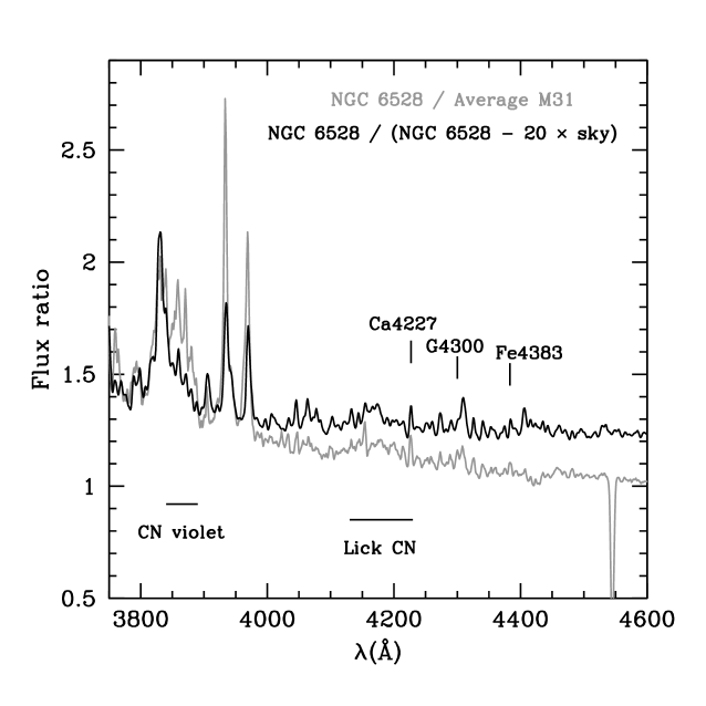
Figure 15: Ratio between the spectra of NGC 6528 and M 31 GCs (gray line), compared to a simulation of the effect of an error in the sky subtraction (black line). The latter is achieved by dividing the spectrum of NGC 6528 by that same spectrum, subtracted of a sky spectrum that is artificially boosted by a factor of 20. The two ratio spectra look somewhat similar, suggesting that the difference between NGC 6528 and 6553 and their M 31 metal-rich counterparts may be partly due to sky-subtraction uncertainties. However, the sky-subtraction error required to match the data is exceedingly high (see text), and it nevertheless cannot match the residuals in the Ca H and K lines.

4 Summary

We present absorption line index measurements taken in integrated spectra of a large number of M 31 and MW GCs, from Caldwell et al. (2009) and Schiavon et al. (2005), respectively. We discuss the conversion of instrumental measurements to a common equivalent system (defined in Schiavon, 2007), as well as the uncertainties in the zero points of these systems.

By comparing measurements of CN indices in old GCs belonging to both data sets, we conclude that, in disagreement with previous work by Burstein et al. (1984), Brodie & Huchra (1990), Davidge (1990), Burstein et al. (2004), Beasley et al. (2004), and Puzia et al. (2005), among others, M 31 and MW GCs of the same [Fe/H] generally have similar CN-band strengths. Because this result disagrees with conclusions by many different groups, we have reanalyzed the data by some of these different authors and suggest that in most cases their conclusions were a result of calibration problems. In particular, the blue Lick CN indices are relatively weak and are very sensitive to flux calibration uncertainties.

We also find that the two MW GCs with [Fe/H] $\mathrel{\hbox{\raise 2.15277pt\hbox{$>$}\hbox to0.0pt{\hss\lower 2.15277pt\hbox{$\sim$}}}}-0.4$, NGC 6528 and 6553, have weaker CN bands than their M 31 counterparts at the same [Fe/H]. It is not entirely clear whether this latter difference is real or a by-product of sky-subtraction errors, or of issues with the sampling of the GCs’ brightest stars. Other data sets (e.g., Puzia et al., 2005) do not show similar CN discrepancies between these GCs and their M 31 metal-rich counterparts. Even if our results are correct, and these two GCs indeed have weaker CN indices than metal-rich M 31 GCs, the fact that they seem to depart significantly from a $\langle$Fe$\rangle$–$CN_{1}$ trend that is present in both samples suggests that NGC 6528 and 6553 are the exception rather than the rule.

The result by Burstein et al. (1984) that M 31 GCs have stronger CN bands than their MW counterparts of same metallicity, even though confirmed by several later studies, has always been difficult to understand because it is very hard to explain how nitrogen abundances could differ substantially between otherwise very similar systems. Li & Burstein (2003) proposed a scenario where GCs were formed from zero-metallicity material, pre-enriched by hypernovae explosions in the center of $\sim 10^{6}M_{\odot}$ gas clouds. Nitrogen abundance differences between the two GC systems was the one piece of evidence that could not be explained in that scenario. We hope that the task of devising a mechanism for the formation of the haloes of the Milky Way and Andromeda galaxies is made easier by the findings presented in this paper. In a forthcoming paper, we contrast measurements of the abundance patterns of M 31 and Galactic GCs, and discuss their implications to our understanding of the formation of the two galaxy haloes.

Table 1: Zero-point conversions between the equivalent width system of the Tololo spectra of MW globular clusters and the Lick indices from Schiavon (2007)

Index	$H\delta_{A}$	$H\delta_{F}$	CN1	CN2	Ca4227	G4300	$H\gamma_{A}$	$H\gamma_{F}$	Fe4383	C24668	$H\beta$	Mg2	Mg $b$	Fe5270	Fe5335
Zero point1 (${\rm\AA}$)	+0.08	–0.03	–0.0088	–0.0065	–0.03	–0.28	+0.45	+0.10	–0.09	+0.28	–0.04	–0.019	–0.14	–0.07	–0.09
r.m.s. (${\rm\AA}$)	0.25	0.12	0.011	0.0081	0.04	0.20	0.46	0.22	0.27	0.13	0.08	0.015	0.15	0.14	0.08

Table 2: Zero-point conversions between the equivalent width system of the Hectospec spectra of M 31 clusters and the Lick indices from Schiavon (2007)

Index	$H\delta_{A}$	$H\delta_{F}$	CN1	CN2	Ca4227	G4300	$H\gamma_{A}$	$H\gamma_{F}$	Fe4383	C24668	$H\beta$	Fe5015	Mg2	Mg $b$	Fe5270	Fe5335
Zero point1 (${\rm\AA}$)	–0.25	–0.06	+0.0054	+0.0054	+0.01	–0.01	+0.01	–0.01	+0.12	–0.04	+0.04	–0.03	–0.0086	–0.07	+0.04	–0.04
r.m.s. (${\rm\AA}$)	0.26	0.10	0.008	0.011	0.10	0.13	0.18	0.09	0.24	0.41	0.14	0.17	0.005	0.15	0.13	0.11

Table 3: M 31 clusters used in the calculation of mean spectra for comparison with MW globular clusters

NGC 2298	NGC 1851	47 Tuc	NGC 6441	NGC 6528
B003-G045	B011-G063	B001-G039	B001-G039	B055-G116
B010-G062	B027-G087	B005-G052	B004-G050	B056-G117
B022-G074	B058-G119	B016-G066	B005-G052	B143-G198
B085-G147	B076-G138	B024-G082	B008-G060	B144-G000
B165-G218	B083-G146	B034-G096	B013-G065	B147-G199
B176-G227	B148-G200	B036-G000	B016-G066	B163-G217
B188-G239	B159-G000	B037-G000	B019-G072	B193-G244
B237-G299	B161-G215	B039-G101	B034-G096
B317-G041	B178-G229	B045-G108	B035-G000
B366-G291	B201-G250	B048-G110	B044-G107
B396-G335	B206-G257	B051-G114	B091D-D058
B399-G342	B221-G276	B077-G139	B103D-G245
	B291-G009	B098-G000	B123-G182
	B312-G035	B106-G168	B124-G000
	B338-G076	B116-G178	B127-G185
	B372-G304	B152-G207	B128-G187
	B397-G336	B158-G213	B151-G205
		B170-G221	B152-G207
		B185-G235	B170-G221
		B203-G252	B204-G254
		B213-G264	B225-G280
		B228-G281	B228-G281
		B234-G290	B234-G290
		B238-G301	B238-G301
		B246-G000	B348-G153
		B283-G296	B384-G319
		B301-G022
		B348-G153
		B383-G318
		B384-G319
		B461-G131

Table 4: Lick indices and uncertainties for standard stars observed with MMT/Hectospec

ID	$H\delta_{A}$	$H\delta_{F}$	$CN_{1}$	$CN_{2}$	Ca4227	G4300	$H\gamma_{A}$	$H\gamma_{F}$	Fe4383	Ca4455	Fe4531	$C_{2}4668$	$H\beta$
HD 41597	-4.49	-1.13	0.136	0.165	0.58	6.96	-8.39	-2.93	4.50	1.29	3.37	4.23	1.38
	0.06	0.04	0.001	0.002	0.03	0.04	0.05	0.03	0.06	0.03	0.04	0.06	0.02
HD 41597	-4.57	-1.19	0.136	0.167	0.58	6.92	-8.31	-2.87	4.44	1.27	3.38	4.34	1.36
	0.05	0.04	0.001	0.002	0.03	0.04	0.05	0.03	0.05	0.03	0.04	0.06	0.02
HD 41597	-4.54	-1.05	0.140	0.170	0.56	6.85	-8.33	-2.89	4.46	1.26	3.44	4.47	1.36
	0.06	0.04	0.001	0.002	0.03	0.04	0.05	0.03	0.06	0.03	0.04	0.06	0.02
HD 43380	-6.23	-1.49	0.264	0.305	1.03	6.54	-9.33	-3.20	6.12	1.72	3.65	8.45	1.50
	0.10	0.07	0.003	0.003	0.05	0.07	0.08	0.05	0.09	0.05	0.07	0.09	0.04
HD 43380	-6.13	-1.45	0.261	0.300	0.97	6.56	-9.49	-3.22	6.36	1.76	3.64	8.65	1.41
	0.09	0.06	0.002	0.003	0.04	0.06	0.07	0.04	0.08	0.04	0.06	0.08	0.03
HD 43380	-5.97	-1.34	0.258	0.296	0.98	6.63	-9.48	-3.20	6.33	1.77	3.77	8.48	1.35
	0.08	0.05	0.002	0.002	0.04	0.05	0.06	0.04	0.07	0.04	0.05	0.07	0.03
HD 50420	8.47	5.88	-0.172	-0.140	0.22	-0.73	7.52	6.22	0.04	0.24	1.62	0.09	6.49
	0.03	0.02	0.001	0.001	0.02	0.04	0.03	0.02	0.05	0.03	0.04	0.06	0.02
HD 50420	8.47	5.88	-0.171	-0.139	0.18	-0.73	7.54	6.24	0.13	0.22	1.64	0.14	6.53
	0.03	0.02	0.001	0.001	0.02	0.03	0.03	0.02	0.05	0.03	0.04	0.06	0.02
HD 50420	8.47	5.84	-0.172	-0.140	0.21	-0.78	7.54	6.24	0.10	0.26	1.65	0.19	6.48
	0.03	0.02	0.001	0.001	0.02	0.03	0.03	0.02	0.05	0.02	0.04	0.06	0.02
HD204642	-6.30	-1.44	0.209	0.245	1.17	6.37	-9.68	-3.18	6.87	1.71	3.84	7.62	1.38
	0.13	0.08	0.003	0.004	0.06	0.08	0.10	0.06	0.11	0.06	0.08	0.12	0.05
HD204642	-6.43	-1.44	0.211	0.246	1.23	6.43	-9.48	-3.08	6.88	1.69	3.77	7.59	1.37
	0.13	0.08	0.003	0.004	0.06	0.08	0.10	0.06	0.11	0.06	0.09	0.12	0.05
HD204642	-6.18	-1.33	0.205	0.239	1.16	6.37	-9.69	-3.11	7.10	1.75	3.87	7.51	1.50
	0.13	0.09	0.003	0.004	0.06	0.09	0.11	0.07	0.12	0.06	0.09	0.12	0.05
HD210855	2.97	2.50	-0.081	-0.058	0.47	3.28	0.50	2.27	1.61	0.61	2.33	2.15	3.85
	0.03	0.02	0.001	0.001	0.02	0.03	0.03	0.02	0.04	0.02	0.03	0.04	0.02
HD210855	2.98	2.54	-0.080	-0.058	0.46	3.23	0.51	2.33	1.71	0.60	2.31	2.08	3.84
	0.04	0.03	0.001	0.001	0.02	0.04	0.04	0.02	0.06	0.03	0.04	0.07	0.02
HD210855	2.91	2.50	-0.077	-0.055	0.49	3.27	0.52	2.30	1.70	0.63	2.27	2.09	3.82
	0.03	0.02	0.001	0.001	0.02	0.03	0.03	0.02	0.05	0.03	0.04	0.06	0.02
HD218470	4.46	3.42	-0.099	-0.072	0.36	1.56	3.11	3.56	0.76	0.40	1.93	0.82	4.33
	0.02	0.02	0.001	0.001	0.02	0.03	0.02	0.01	0.04	0.02	0.03	0.05	0.02
HD218470	4.40	3.41	-0.098	-0.073	0.37	1.66	2.98	3.52	0.78	0.42	2.04	0.81	4.32
	0.07	0.05	0.002	0.003	0.04	0.07	0.07	0.04	0.11	0.06	0.08	0.13	0.05
HD218470	4.46	3.40	-0.097	-0.069	0.37	1.60	3.03	3.52	0.73	0.41	1.89	0.78	4.33
	0.03	0.02	0.001	0.001	0.02	0.03	0.03	0.02	0.05	0.03	0.04	0.06	0.02
HD218470	4.44	3.41	-0.096	-0.068	0.37	1.61	3.04	3.53	0.79	0.46	1.94	0.80	4.31
	0.03	0.02	0.001	0.001	0.02	0.04	0.03	0.02	0.05	0.03	0.04	0.07	0.02

Table 5: Lick indices and uncertainties for standard stars observed with MMT/Hectospec, continued

ID	Fe5015	Mg1	Mg2	Mg $b$	Fe5270	Fe5335	Fe5406	Fe5709	Fe5782	$Na_{D}$	$TiO_{1}$	$TiO_{2}$
HD41597	5.11	0.0699	0.1441	2.19	2.78	2.28	1.51	1.02	0.68	1.58	0.0093	0.0181
	0.05	0.0005	0.0006	0.02	0.02	0.03	0.02	0.01	0.01	0.02	0.0004	0.0004
HD41597	5.10	0.0706	0.1430	2.18	2.80	2.22	1.52	1.03	0.68	1.58	0.0091	0.0174
	0.04	0.0005	0.0005	0.02	0.02	0.03	0.02	0.01	0.01	0.02	0.0004	0.0003
HD41597	5.10	0.0717	0.1442	2.19	2.76	2.26	1.51	0.99	0.67	1.56	0.0097	0.0185
	0.05	0.0005	0.0006	0.02	0.02	0.03	0.02	0.02	0.01	0.02	0.0004	0.0004
HD43380	6.08	0.1393	0.2583	3.83	3.57	3.08	2.13	1.31	1.10	2.61	0.0109	0.0309
	0.07	0.0008	0.0009	0.04	0.04	0.04	0.03	0.02	0.02	0.03	0.0007	0.0006
HD43380	6.15	0.1398	0.2607	3.86	3.60	3.11	2.12	1.33	1.05	2.56	0.0118	0.0310
	0.06	0.0007	0.0008	0.03	0.03	0.04	0.03	0.02	0.02	0.02	0.0006	0.0005
HD43380	6.19	0.1399	0.2584	3.81	3.58	3.18	2.15	1.34	1.08	2.56	0.0105	0.0308
	0.06	0.0006	0.0008	0.03	0.03	0.03	0.03	0.02	0.02	0.02	0.0005	0.0005
HD50420	2.55	0.0081	0.0358	0.48	1.20	0.80	0.29	0.19	0.16	1.06	0.0047	0.0042
	0.05	0.0005	0.0006	0.03	0.03	0.03	0.03	0.02	0.02	0.03	0.0006	0.0005
HD50420	2.57	0.0073	0.0370	0.51	1.15	0.81	0.28	0.17	0.19	1.04	0.0061	0.0042
	0.05	0.0005	0.0006	0.02	0.03	0.03	0.03	0.02	0.02	0.02	0.0006	0.0005
HD50420	2.41	0.0088	0.0351	0.51	1.11	0.78	0.25	0.16	0.15	1.02	0.0057	0.0044
	0.05	0.0005	0.0006	0.02	0.03	0.03	0.02	0.02	0.02	0.02	0.0005	0.0005
HD204642	5.95	0.1131	0.2420	3.83	3.70	3.10	2.23	1.32	0.96	2.86	0.0152	0.0227
	0.10	0.0011	0.0013	0.05	0.05	0.06	0.04	0.03	0.03	0.04	0.0009	0.0008
HD204642	5.70	0.1107	0.2429	3.82	3.60	3.14	2.15	1.27	1.03	2.92	0.0152	0.0216
	0.10	0.0011	0.0013	0.05	0.05	0.06	0.05	0.03	0.03	0.04	0.0010	0.0008
HD204642	5.82	0.1119	0.2431	3.85	3.83	3.19	2.10	1.36	1.02	2.80	0.0142	0.0225
	0.10	0.0011	0.0013	0.05	0.05	0.06	0.05	0.03	0.03	0.04	0.0010	0.0008
HD210855	3.93	0.0180	0.0645	1.18	1.63	1.26	0.66	0.55	0.26	0.93	0.0079	0.0048
	0.04	0.0004	0.0004	0.02	0.02	0.02	0.02	0.01	0.01	0.02	0.0004	0.0003
HD210855	3.92	0.0175	0.0648	1.19	1.60	1.33	0.63	0.53	0.30	0.96	0.0082	0.0031
	0.05	0.0006	0.0007	0.03	0.03	0.04	0.03	0.02	0.02	0.03	0.0006	0.0005
HD210855	3.85	0.0182	0.0656	1.18	1.68	1.32	0.70	0.54	0.30	0.93	0.0075	0.0044
	0.05	0.0005	0.0006	0.02	0.03	0.03	0.02	0.02	0.02	0.02	0.0005	0.0005
HD218470	2.76	0.0144	0.0472	0.89	1.20	0.99	0.41	0.32	0.11	0.58	0.0040	0.0036
	0.04	0.0004	0.0005	0.02	0.02	0.03	0.02	0.01	0.01	0.02	0.0004	0.0004
HD218470	2.92	0.0158	0.0482	0.94	1.23	0.94	0.49	0.27	0.13	0.65	0.0042	0.0034
	0.11	0.0011	0.0013	0.05	0.06	0.07	0.05	0.04	0.04	0.05	0.0012	0.0010
HD218470	2.78	0.0140	0.0482	0.92	1.17	1.03	0.45	0.28	0.14	0.59	0.0055	0.0035
	0.05	0.0005	0.0006	0.02	0.03	0.03	0.02	0.02	0.02	0.02	0.0005	0.0005
HD218470	2.72	0.0137	0.0481	0.86	1.18	0.96	0.45	0.32	0.11	0.64	0.0049	0.0036
	0.06	0.0006	0.0007	0.03	0.03	0.04	0.03	0.02	0.02	0.03	0.0006	0.0006

Table 6: Lick indices for standard stars observed at CTIO

ID	$H\delta_{A}$	$H\delta_{F}$	$CN_{1}$	$CN_{2}$	Ca4227	G4300	$H\gamma_{A}$	$H\gamma_{F}$	Fe4383	Ca4455	Fe4531	$C_{2}4668$	$H\beta$
HD 76151	-0.77	0.82	-0.030	-0.016	0.77	4.85	-3.85	-0.33	3.52	0.84	6.54	3.89	2.67
HD 76924	-4.59	-1.31	0.196	0.224	0.40	6.28	-7.64	-2.20	4.80	1.30	7.16	5.51	1.58
HD 78558	-0.50	0.92	-0.035	-0.022	0.63	5.01	-3.88	-0.37	3.36	0.76	6.37	3.62	2.55
HD102574	1.79	1.92	-0.068	-0.051	0.59	3.95	-1.24	1.27	2.35	0.78	6.52	3.30	3.34
HD157881	-2.45	-0.02	-0.088	-0.053	4.24	3.74	-7.76	-2.71	5.80	1.67	9.66	0.47	-0.82
HD 76151	-0.68	0.91	-0.033	-0.017	0.73	4.78	-3.89	-0.35	3.58	0.82	6.83	3.79	2.67
HD157881	-2.51	-0.05	-0.088	-0.053	4.25	4.01	-8.01	-2.93	5.63	1.66	10.16	0.58	-0.91

Table 7: Lick indices for standard stars observed at CTIO. The Fe5015 index could not be measured in the CTIO sample, because of the presence of a group of bad CCD columns crossing the spectra within the index passband.

ID	Mg1	Mg2	Mg $b$	Fe5270	Fe5335	Fe5406	Fe5709	Fe5782	$Na_{D}$	$TiO_{1}$	$TiO_{2}$
HD 76151	0.0191	0.1303	3.00	2.27	1.86	1.07	0.76	0.44	1.77	-0.0429	-0.0411
HD 76924	0.0374	0.1246	2.09	2.90	2.34	1.62	1.11	0.75	1.96	-0.0405	-0.0122
HD 78558	0.0209	0.1156	2.70	2.31	1.76	0.97	0.70	0.45	1.73	-0.0465	-0.0286
HD102574	0.0074	0.0779	1.70	1.91	1.58	0.80	0.67	0.36	1.09	-0.0461	-0.0184
HD157881	0.3540	0.4627	4.34	4.50	4.43	3.10	0.70	0.95	10.34	-0.0164	0.0916
HD 76151	0.0156	0.1271	3.05	2.25	1.86	1.00	0.73	0.42	1.63	-0.0472	0.0082
HD157881	0.3521	0.4670	4.41	4.56	4.46	3.10	0.74	0.98	10.35	-0.0210	0.1036

Table 8: Lick indices and uncertainties for Galactic globular clusters from Schiavon et al. (2005)

ID	$H\delta_{A}$	$H\delta_{F}$	$CN_{1}$	$CN_{2}$	Ca4227	G4300	$H\gamma_{A}$	$H\gamma_{F}$	Fe4383	Ca4455	$C_{2}4668$	$H\beta$
NGC104	-0.48	0.68	0.025	0.050	0.56	4.66	-4.27	-0.66	2.49	0.67	1.68	1.60
	0.02	0.02	0.001	0.001	0.01	0.02	0.02	0.01	0.03	0.02	0.03	0.01
NGC1851	2.23	2.06	-0.056	-0.031	0.34	2.79	-0.60	1.23	1.28	0.43	0.57	2.27
	0.04	0.02	0.001	0.001	0.02	0.04	0.03	0.02	0.05	0.03	0.06	0.02
NGC1904	3.17	2.61	-0.085	-0.062	0.21	1.89	0.87	1.88	0.70	0.23	-0.07	2.48
	0.06	0.04	0.002	0.002	0.04	0.06	0.06	0.04	0.09	0.05	0.11	0.04
NGC2298	3.70	2.87	-0.102	-0.079	0.24	1.66	1.45	2.13	0.65	0.15	0.17	2.68
	0.09	0.07	0.003	0.004	0.06	0.10	0.09	0.06	0.14	0.07	0.16	0.06
NGC2808	1.57	1.65	-0.047	-0.024	0.42	2.88	-1.28	0.83	1.56	0.42	0.57	2.03
	0.14	0.10	0.004	0.005	0.08	0.14	0.13	0.08	0.20	0.10	0.22	0.08
NGC3201	2.77	2.27	-0.087	-0.063	0.36	2.30	-0.04	1.41	1.35	0.39	-0.44	2.49
	0.13	0.09	0.004	0.005	0.08	0.40	0.29	0.12	0.19	0.10	0.21	0.08
NGC5286	3.27	2.57	-0.086	-0.064	0.23	2.08	0.65	1.75	0.76	0.23	0.03	2.44
	0.07	0.05	0.002	0.003	0.04	0.07	0.07	0.04	0.11	0.06	0.12	0.05
NGC5904	2.97	2.51	-0.079	-0.055	0.34	2.26	0.28	1.60	0.99	0.33	0.29	2.43
	0.05	0.03	0.001	0.002	0.03	0.04	0.04	0.03	0.07	0.03	0.07	0.03
NGC5927	-1.22	0.27	0.039	0.066	0.74	4.79	-5.18	-1.10	3.61	0.93	2.65	1.41
	0.18	0.13	0.005	0.006	0.09	0.15	0.16	0.10	0.21	0.11	0.22	0.08
NGC5946	3.29	2.58	-0.088	-0.067	0.22	2.24	0.42	1.70	0.97	0.15	-0.37	2.44
	0.10	0.07	0.003	0.004	0.06	0.39	0.28	0.10	0.13	0.07	0.14	0.05
NGC5986	3.25	2.66	-0.085	-0.062	0.27	1.81	0.80	1.88	0.90	0.19	0.01	2.50
	0.04	0.03	0.001	0.001	0.02	0.04	0.04	0.02	0.06	0.03	0.06	0.02
NGC6121	2.85	2.34	-0.071	-0.049	0.32	2.50	0.00	1.40	1.27	0.33	0.32	2.28
	0.06	0.04	0.002	0.002	0.04	0.06	0.06	0.04	0.09	0.05	0.10	0.04
NGC6171	1.35	1.41	-0.049	-0.022	0.43	3.80	-2.28	0.36	2.00	0.51	1.01	2.08
	0.14	0.10	0.004	0.005	0.08	0.12	0.13	0.08	0.17	0.09	0.18	0.07
NGC6218	3.18	2.64	-0.090	-0.067	0.31	2.30	0.45	1.65	0.78	0.23	-0.11	2.45
	0.03	0.02	0.001	0.001	0.02	0.03	0.03	0.02	0.04	0.02	0.05	0.02
NGC6235	2.83	2.35	-0.060	-0.035	0.34	2.76	-0.77	1.17	1.58	0.37	0.90	2.26
	0.02	0.01	0.001	0.001	0.01	0.02	0.02	0.01	0.03	0.02	0.04	0.01
NGC6254	2.78	2.26	-0.080	-0.058	0.27	2.34	-0.05	1.40	1.03	0.24	-0.20	2.23
	0.11	0.07	0.003	0.004	0.05	0.09	0.09	0.06	0.12	0.06	0.12	0.05
NGC6266	1.88	1.88	-0.044	-0.021	0.37	2.95	-0.96	1.00	1.55	0.38	0.56	2.12
	0.12	0.09	0.003	0.004	0.06	0.10	0.11	0.07	0.13	0.07	0.14	0.05
NGC62841	2.60	2.36	-0.062	-0.038	0.35	2.53	-0.15	1.45	1.34	0.37	0.41	2.35
	0.11	0.08	0.003	0.004	0.06	0.09	0.10	0.06	0.12	0.06	0.12	0.05
NGC62842	2.44	2.26	-0.058	-0.033	0.36	2.60	-0.39	1.31	1.41	0.39	0.54	2.25
	0.13	0.09	0.004	0.005	0.07	0.12	0.12	0.07	0.17	0.09	0.19	0.07
NGC6304	-0.91	0.34	0.037	0.063	0.70	4.84	-5.08	-1.05	3.38	0.83	2.35	1.49
	0.05	0.03	0.001	0.002	0.03	0.05	0.04	0.03	0.07	0.04	0.08	0.03
NGC6316	0.10	0.80	-0.015	0.007	0.61	4.48	-3.97	-0.57	2.69	0.66	1.16	1.50
	0.11	0.08	0.003	0.004	0.06	0.10	0.10	0.06	0.14	0.07	0.15	0.06
NGC6333	3.57	2.78	-0.093	-0.070	0.22	1.59	1.15	1.99	0.68	0.19	-0.10	2.56
	0.14	0.10	0.004	0.005	0.08	0.12	0.13	0.08	0.17	0.09	0.18	0.07
NGC63421	0.29	0.85	-0.020	-0.002	0.50	4.29	-3.37	-0.34	2.65	0.66	1.40	2.04
	0.14	0.10	0.004	0.005	0.07	0.12	0.12	0.08	0.17	0.09	0.17	0.07
NGC63422	-0.11	0.73	-0.004	0.019	0.56	4.51	-3.88	-0.53	2.82	0.73	1.56	1.86
	0.06	0.04	0.002	0.002	0.04	0.06	0.06	0.04	0.09	0.05	0.10	0.04
NGC6352	-0.15	0.78	0.002	0.027	0.70	5.73	-5.38	-1.25	3.28	0.73	2.17	1.33
	0.19	0.14	0.006	0.007	0.11	0.18	0.18	0.11	0.25	0.13	0.26	0.10
NGC6356	-0.54	0.56	0.017	0.042	0.64	4.72	-4.39	-0.72	2.86	0.75	1.73	1.60
	0.05	0.04	0.002	0.002	0.03	0.05	0.05	0.03	0.07	0.04	0.08	0.03
NGC6362	1.74	1.64	-0.067	-0.042	0.48	3.45	-1.64	0.58	1.56	0.41	0.39	1.97
	0.03	0.02	0.001	0.001	0.02	0.03	0.03	0.02	0.04	0.02	0.04	0.02
NGC6388	0.15	0.98	0.019	0.045	0.51	4.01	-3.34	-0.05	2.95	0.73	1.90	1.87
	0.06	0.04	0.002	0.002	0.04	0.06	0.06	0.04	0.09	0.05	0.10	0.04
NGC64411	0.17	0.98	0.023	0.049	0.58	4.02	-3.50	-0.12	3.06	0.77	1.92	1.81
	0.05	0.04	0.002	0.002	0.03	0.05	0.05	0.03	0.08	0.04	0.08	0.03
NGC64412	0.15	0.93	0.020	0.047	0.58	4.00	-3.54	-0.15	3.05	0.77	1.91	1.80
	0.10	0.07	0.003	0.003	0.05	0.08	0.09	0.05	0.11	0.06	0.11	0.04
NGC6522	2.79	2.39	-0.061	-0.036	0.29	2.62	-0.37	1.33	1.39	0.36	0.47	2.21
	0.12	0.09	0.003	0.004	0.07	0.11	0.11	0.07	0.15	0.08	0.15	0.06
NGC65281	-1.36	0.37	0.059	0.088	0.88	4.81	-5.75	-1.27	4.58	1.16	4.41	1.59
	0.21	0.15	0.006	0.007	0.11	0.17	0.19	0.11	0.23	0.12	0.24	0.09
NGC65282	-1.45	0.30	0.063	0.093	0.89	4.82	-5.79	-1.31	4.67	1.17	4.51	1.57
	0.17	0.12	0.005	0.006	0.09	0.14	0.15	0.09	0.19	0.10	0.19	0.08
NGC6544	1.85	1.49	-0.056	-0.038	0.34	2.90	-1.48	0.53	1.47	0.40	0.33	1.60
	0.19	0.13	0.005	0.006	0.10	0.16	0.17	0.11	0.24	0.12	0.26	0.10
NGC6553	-0.91	0.33	0.042	0.071	0.69	4.68	-5.11	-1.03	3.87	0.92	3.95	1.56
	0.16	0.11	0.004	0.005	0.08	0.13	0.14	0.09	0.19	0.10	0.20	0.07
NGC6569	0.95	1.12	-0.044	-0.020	0.51	3.81	-2.60	0.10	1.91	0.48	0.99	1.74
	0.06	0.04	0.002	0.002	0.03	0.05	0.06	0.04	0.08	0.04	0.10	0.04
NGC66241	-0.33	0.71	0.017	0.043	0.55	4.54	-4.11	-0.50	2.89	0.75	1.77	1.68
	0.06	0.04	0.002	0.002	0.03	0.05	0.06	0.04	0.08	0.04	0.08	0.03
NGC66242	-0.42	0.64	0.022	0.048	0.57	4.63	-4.18	-0.55	2.95	0.80	1.78	1.62
	0.08	0.06	0.002	0.003	0.05	0.08	0.08	0.05	0.12	0.06	0.12	0.05
NGC6626	2.88	2.48	-0.068	-0.044	0.30	2.41	-0.02	1.48	1.24	0.36	0.47	2.37
	0.03	0.02	0.001	0.001	0.02	0.03	0.03	0.02	0.04	0.02	0.05	0.02
NGC6637	-0.12	0.70	-0.009	0.014	0.60	4.76	-4.07	-0.64	2.41	0.69	1.65	1.56
	0.04	0.03	0.001	0.001	0.02	0.04	0.04	0.02	0.05	0.03	0.06	0.02
NGC6638	1.03	1.25	-0.026	-0.001	0.51	4.09	-2.80	0.06	2.06	0.47	1.28	1.77
	0.04	0.03	0.001	0.001	0.02	0.03	0.03	0.02	0.05	0.02	0.05	0.02
NGC6652	1.10	1.37	-0.040	-0.017	0.43	4.34	-2.70	0.05	1.97	0.48	1.06	2.03
	0.08	0.06	0.003	0.003	0.05	0.08	0.08	0.05	0.12	0.06	0.13	0.05
NGC6723	2.02	1.88	-0.057	-0.033	0.30	3.06	-0.96	0.97	1.29	0.32	0.34	2.14
	0.13	0.09	0.004	0.004	0.06	0.10	0.11	0.07	0.14	0.07	0.14	0.05
NGC6752	3.22	2.69	-0.085	-0.061	0.20	1.99	0.91	1.93	0.66	0.22	0.08	2.59
	0.14	0.09	0.004	0.004	0.07	0.11	0.12	0.07	0.15	0.08	0.15	0.06
NGC70781	4.07	3.12	-0.100	-0.083	0.11	0.58	2.34	2.54	0.17	0.09	-0.52	2.75
	0.13	0.09	0.004	0.004	0.06	0.10	0.11	0.07	0.13	0.07	0.14	0.05
NGC70782	3.91	3.01	-0.096	-0.080	0.12	0.70	2.12	2.38	0.18	0.12	-0.43	2.67
	0.12	0.08	0.003	0.004	0.06	0.09	0.10	0.06	0.12	0.06	0.12	0.05
NGC7089	3.29	2.67	-0.086	-0.062	0.25	2.00	0.82	1.88	0.69	0.25	0.04	2.54
	0.12	0.08	0.003	0.004	0.06	0.09	0.10	0.06	0.13	0.07	0.13	0.05

Table 9: Lick indices and uncertainties for Galactic globular clusters from Schiavon et al. (2005), continued.

ID	Mg1	Mg2	Mg $b$	Fe5270	Fe5335	Fe5406	Fe5709	Fe5782	$Na_{D}$	$TiO_{1}$	$TiO_{2}$
NGC 104	0.0569	0.1589	2.69	1.91	1.68	1.06	0.64	0.46	1.57	0.0203	0.0581
	0.0003	0.0004	0.01	0.02	0.02	0.01	0.01	0.01	0.01	0.0003	0.0003
NGC1851	0.0251	0.0829	1.35	1.40	1.12	0.67	0.46	0.22	1.21	-0.0169	0.0046
	0.0005	0.0006	0.02	0.03	0.03	0.02	0.02	0.02	0.02	0.0005	0.0005
NGC1904	0.0103	0.0485	0.83	0.93	0.78	0.34	0.22	0.12	0.90	-0.0111	-0.0003
	0.0009	0.0011	0.05	0.05	0.06	0.04	0.04	0.03	0.05	0.0010	0.0009
NGC2298	0.0070	0.0442	0.79	0.74	0.63	0.24	0.18	0.18	1.96	-0.0122	0.0005
	0.0013	0.0016	0.07	0.07	0.08	0.06	0.05	0.05	0.07	0.0014	0.0013
NGC2808	0.0231	0.0844	1.33	1.41	1.16	0.70	0.51	0.35	1.46	0.0098	0.0224
	0.0018	0.0021	0.09	0.10	0.11	0.08	0.07	0.07	0.10	0.0020	0.0017
NGC3201	0.0079	0.0617	1.14	1.09	0.89	0.58	0.32	0.03	3.89	-0.0037	-0.0217
	0.0017	0.0019	0.08	0.09	0.10	0.07	0.06	0.06	0.08	0.0017	0.0015
NGC5286	0.0149	0.0585	0.96	0.92	0.80	0.38	0.30	0.23	1.73	-0.0052	0.0077
	0.0010	0.0012	0.05	0.05	0.06	0.05	0.04	0.03	0.05	0.0010	0.0009
NGC5904	0.0212	0.0759	1.25	1.20	1.01	0.56	0.41	0.20	0.82	0.0039	0.0150
	0.0006	0.0007	0.03	0.03	0.04	0.03	0.02	0.02	0.03	0.0006	0.0006
NGC5927	0.0759	0.2029	3.42	2.33	1.98	1.25	0.87	0.85	4.45	0.0233	0.0648
	0.0017	0.0021	0.08	0.09	0.10	0.07	0.06	0.05	0.08	0.0016	0.0014
NGC5946	0.0243	0.0649	0.89	0.97	0.64	0.37	0.42	0.32	3.00	-0.0109	-0.0098
	0.0011	0.0013	0.05	0.06	0.07	0.05	0.04	0.04	0.05	0.0011	0.0009
NGC5986	0.0129	0.0572	0.92	0.89	0.72	0.39	0.32	0.21	2.59	0.0008	-0.0016
	0.0005	0.0006	0.02	0.03	0.03	0.02	0.02	0.02	0.02	0.0005	0.0005
NGC6121	0.0245	0.0883	1.58	1.21	0.98	0.57	0.47	0.35	1.79	0.0211	0.0103
	0.0008	0.0010	0.04	0.05	0.05	0.04	0.03	0.03	0.04	0.0009	0.0008
NGC6171	0.0396	0.1191	2.05	1.57	1.24	0.71	0.51	0.48	1.66	0.0130	0.0136
	0.0014	0.0016	0.06	0.07	0.08	0.06	0.04	0.04	0.06	0.0012	0.0011
NGC6218	0.0162	0.0706	1.29	1.04	0.81	0.41	0.33	0.33	0.66	-0.0045	0.0034
	0.0004	0.0005	0.02	0.02	0.02	0.02	0.01	0.01	0.02	0.0004	0.0004
NGC6235	0.0244	0.0862	1.16	1.41	1.18	0.66	0.65	0.42	3.38	-0.0113	0.0140
	0.0003	0.0004	0.01	0.02	0.02	0.01	0.01	0.01	0.01	0.0003	0.0003
NGC6254	0.0135	0.0594	0.90	0.95	0.76	0.36	0.35	0.26	1.32	0.0073	0.0126
	0.0009	0.0011	0.04	0.05	0.05	0.04	0.03	0.03	0.04	0.0008	0.0007
NGC6266	0.0240	0.0902	1.54	1.34	1.12	0.64	0.51	0.49	2.35	0.0023	0.0139
	0.0011	0.0013	0.05	0.05	0.06	0.04	0.03	0.03	0.04	0.0009	0.0008
NGC62841	0.0258	0.0916	1.50	1.26	1.03	0.61	0.45	0.39	2.03	-0.0101	0.0111
	0.0010	0.0012	0.04	0.05	0.05	0.04	0.03	0.03	0.04	0.0009	0.0008
NGC62842	0.0305	0.0966	1.52	1.32	1.07	0.66	0.50	0.42	2.12	-0.0082	0.0081
	0.0014	0.0016	0.06	0.07	0.08	0.06	0.04	0.04	0.05	0.0012	0.0010
NGC6304	0.0664	0.1835	3.17	2.15	1.82	1.13	0.82	0.81	3.74	0.0149	0.0276
	0.0006	0.0007	0.03	0.03	0.04	0.03	0.02	0.02	0.03	0.0006	0.0006
NGC6316	0.0544	0.1547	2.54	1.83	1.44	0.96	0.78	0.71	4.63	0.0051	0.0392
	0.0011	0.0013	0.05	0.06	0.07	0.05	0.04	0.03	0.05	0.0010	0.0009
NGC6333	0.0149	0.0500	0.78	0.78	0.60	0.33	0.22	0.04	1.89	0.0003	-0.0207
	0.0013	0.0016	0.06	0.07	0.08	0.06	0.04	0.04	0.06	0.0012	0.0010
NGC63421	0.0274	0.1213	2.47	1.57	1.45	0.72	0.56	0.41	2.68	-0.0068	0.0097
	0.0013	0.0015	0.06	0.07	0.08	0.06	0.04	0.04	0.06	0.0012	0.0010
NGC63422	0.0406	0.1387	2.55	1.76	1.52	0.87	0.63	0.54	2.85	-0.0059	0.0114
	0.0008	0.0010	0.04	0.04	0.05	0.04	0.03	0.03	0.05	0.0009	0.0008
NGC6352	0.0548	0.1607	2.92	1.85	1.71	1.17	0.72	0.65	3.22	-0.0044	0.0142
	0.0020	0.0024	0.10	0.11	0.12	0.09	0.07	0.07	0.11	0.0020	0.0017
NGC6356	0.0640	0.1726	2.87	1.99	1.70	1.09	0.70	0.62	3.53	0.0132	0.0311
	0.0006	0.0007	0.03	0.03	0.04	0.03	0.02	0.02	0.03	0.0006	0.0006
NGC6362	0.0322	0.1098	1.94	1.37	1.03	0.68	0.49	0.33	8.80	0.0256	0.0539
	0.0003	0.0004	0.02	0.02	0.02	0.01	0.01	0.01	0.01	0.0003	0.0003
NGC6388	0.0489	0.1430	2.20	2.09	1.75	1.16	0.77	0.69	3.65	0.0151	0.0372
	0.0008	0.0010	0.04	0.04	0.05	0.04	0.03	0.03	0.04	0.0008	0.0007
NGC64411	0.0601	0.1640	2.64	2.13	1.79	1.15	0.81	0.79	3.97	0.0046	0.0305
	0.0007	0.0008	0.03	0.04	0.04	0.03	0.02	0.02	0.03	0.0007	0.0006
NGC64412	0.0602	0.1651	2.65	2.13	1.78	1.15	0.81	0.78	3.97	0.0173	0.0349
	0.0009	0.0011	0.04	0.04	0.05	0.04	0.03	0.03	0.03	0.0008	0.0007
NGC6522	0.0394	0.1040	1.48	1.41	1.11	0.68	0.60	0.60	2.89	0.0038	0.0130
	0.0012	0.0014	0.05	0.06	0.07	0.05	0.03	0.03	0.04	0.0010	0.0008
NGC65281	0.1041	0.2515	3.80	2.77	2.42	1.67	1.03	0.80	4.96	0.0313	0.1118
	0.0019	0.0023	0.09	0.09	0.10	0.08	0.06	0.06	0.07	0.0016	0.0015
NGC65282	0.1025	0.2489	3.76	2.80	2.42	1.69	1.01	0.80	5.00	0.0324	0.1087
	0.0015	0.0019	0.07	0.08	0.09	0.06	0.05	0.05	0.06	0.0014	0.0012
NGC6544	0.0413	0.0934	1.00	1.37	1.07	0.65	0.55	0.63	2.14	-0.0079	-0.0053
	0.0020	0.0024	0.09	0.10	0.12	0.09	0.07	0.06	0.08	0.0018	0.0016
NGC6553	0.0944	0.2420	3.82	2.74	2.20	1.68	1.01	1.13	3.59	0.0231	0.0900
	0.0015	0.0018	0.07	0.08	0.09	0.06	0.05	0.05	0.06	0.0014	0.0012
NGC6569	0.0454	0.1341	2.14	1.50	1.30	0.81	0.56	0.55	3.71	0.0083	0.0579
	0.0008	0.0010	0.04	0.04	0.05	0.04	0.03	0.03	0.03	0.0008	0.0007
NGC66241	0.0540	0.1546	2.58	1.94	1.62	1.05	0.72	0.61	2.22	-0.0017	0.0421
	0.0007	0.0008	0.03	0.04	0.04	0.03	0.02	0.02	0.03	0.0006	0.0006
NGC66242	0.0522	0.1537	2.56	1.96	1.61	1.04	0.75	0.63	2.23	-0.0031	0.0369
	0.0010	0.0012	0.05	0.06	0.07	0.05	0.04	0.04	0.07	0.0012	0.0011
NGC6626	0.0229	0.0906	1.49	1.15	1.05	0.57	0.47	0.40	1.79	0.0147	0.0393
	0.0004	0.0004	0.02	0.02	0.02	0.02	0.01	0.01	0.01	0.0004	0.0003
NGC6637	0.0498	0.1526	2.51	1.76	1.47	0.97	0.59	0.43	2.97	0.0201	0.0656
	0.0005	0.0005	0.02	0.02	0.03	0.02	0.01	0.01	0.02	0.0004	0.0004
NGC6638	0.0429	0.1311	2.03	1.64	1.34	0.89	0.60	0.61	2.76	0.0070	0.0536
	0.0004	0.0005	0.02	0.02	0.02	0.02	0.01	0.01	0.01	0.0004	0.0003
NGC6652	0.0253	0.1080	2.06	1.50	1.27	0.68	0.53	0.41	1.97	-0.0175	0.0031
	0.0011	0.0013	0.05	0.06	0.07	0.05	0.04	0.04	0.05	0.0011	0.0010
NGC6723	0.0188	0.0830	1.46	1.17	0.91	0.53	0.41	0.24	4.32	-0.0118	0.0027
	0.0011	0.0013	0.05	0.05	0.06	0.04	0.03	0.03	0.04	0.0009	0.0008
NGC6752	0.0109	0.0535	0.94	0.87	0.74	0.32	0.24	0.15	0.76	-0.0049	0.0167
	0.0012	0.0014	0.06	0.06	0.07	0.05	0.04	0.04	0.05	0.0010	0.0009
NGC70781	0.0089	0.0372	0.56	0.48	0.46	0.10	0.05	0.14	1.57	0.0036	-0.0129
	0.0011	0.0014	0.05	0.05	0.06	0.04	0.03	0.03	0.04	0.0009	0.0009
NGC70782	0.0085	0.0369	0.59	0.50	0.45	0.14	0.08	0.12	1.58	-0.0027	-0.0203
	0.0010	0.0012	0.04	0.05	0.05	0.04	0.03	0.03	0.03	0.0008	0.0007
NGC7089	0.0138	0.0568	0.95	0.95	0.80	0.42	0.25	0.15	0.98	-0.0068	-0.0008
	0.0010	0.0012	0.05	0.05	0.06	0.04	0.03	0.03	0.04	0.0009	0.0008

Table 10: Lick indices for M 31 Globular clusters. Sample only. The full table is available in the electronic version.

ID	$CN_{1}$	$CN_{2}$	Ca4227	G4300	Fe4383	Ca4455	Fe4531	$C_{2}4668$	$H\beta$	Fe5015	Mg1
B001-G039	0.003	0.024	0.65	4.92	2.95	0.80	2.48	2.06	1.68	3.48	0.0522
	0.008	0.010	0.15	0.23	0.34	0.16	0.23	0.32	0.12	0.24	0.0023
B002-G043	-0.089	-0.073	0.05	0.82	0.13	0.07	0.66	0.18	2.55	0.53	0.0099
	0.004	0.006	0.09	0.15	0.24	0.11	0.17	0.24	0.09	0.20	0.0020
B003-G045	-0.075	-0.057	0.25	1.74	0.71	0.19	1.31	0.30	2.68	1.33	0.0161
	0.005	0.007	0.10	0.17	0.29	0.13	0.19	0.28	0.11	0.23	0.0023
B004-G050	0.014	0.035	0.56	4.14	2.55	0.76	2.63	2.45	1.78	3.47	0.0478
	0.005	0.006	0.09	0.14	0.22	0.11	0.15	0.22	0.09	0.18	0.0018
B005-G052	0.042	0.066	0.65	4.47	2.43	0.51	2.51	2.10	1.48	3.69	0.0561
	0.005	0.006	0.10	0.15	0.23	0.12	0.17	0.25	0.10	0.21	0.0021

Table 11: Lick indices for M 31 Globular Clusters. Sample only. The full table is available in the electronic version.

ID	Mg2	Mg $b$	Fe5270	Fe5335	Fe5406	Fe5709	Fe5782	$Na_{D}$	$TiO_{1}$	$TiO_{2}$
B001-G039	0.1604	2.63	2.02	1.68	1.21	0.69	0.65	3.31	0.0262	0.0509
	0.0027	0.11	0.12	0.13	0.10	0.07	0.07	0.09	0.0020	0.0016
B002-G043	0.0410	0.62	0.44	0.59	0.37	0.08	0.14	1.02	0.0094	-0.0029
	0.0023	0.10	0.11	0.13	0.09	0.08	0.08	0.12	0.0022	0.0018
B003-G045	0.0588	0.91	0.87	0.77	0.52	0.41	0.24	1.49	0.0106	-0.0038
	0.0026	0.11	0.12	0.14	0.10	0.09	0.08	0.13	0.0025	0.0020
B004-G050	0.1480	2.27	2.04	1.66	1.13	0.67	0.41	2.06	0.0232	0.0372
	0.0021	0.08	0.09	0.11	0.08	0.06	0.06	0.09	0.0018	0.0015
B005-G052	0.1590	2.51	2.11	1.64	1.11	0.70	0.54	2.94	0.0237	0.0374
	0.0025	0.10	0.11	0.12	0.09	0.07	0.07	0.09	0.0020	0.0017

Table 12: Conversion between Tololo and Indo-US Lick/IDS index systems, for indices not modeled by Schiavon (2007), with associated uncertainties.

Index	Ca4455	Mg1	Fe5406	Fe5709	Fe5782	NaD	$TiO_{1}$	$TiO_{2}$
Conversion1	-0.05	-0.01	-0.02	-0.02	-0.029	0.10	-0.006	-0.02
r.m.s.	0.03	0.02	0.04	0.02	0.008	0.07	0.004	0.03

Table 13: Conversion between Hectospec and Indo-US Lick/IDS index systems, for indices not modeled by Schiavon (2007), with associated uncertainties.

Index	Ca4455	Fe4531	Mg1	Fe5406	Fe5709	Fe5782	NaD	$TiO_{1}$	$TiO_{2}$
Conversion1	0.03	-0.11	0.02	-0.06	-0.03	-0.004	-0.03	-0.002	-0.002
r.m.s.	0.07	0.21	0.01	0.09	0.07	0.036	0.13	0.005	0.005

Table 14: Conversion between Indo-US and standard Lick/IDS index systems, for indices not modeled by Schiavon (2007), with associated uncertainties.

Index	Ca4455	Fe4531	Mg1	Fe5406	Fe5709	Fe5782	NaD	$TiO_{1}$	$TiO_{2}$
Conversion1	-0.28	-0.05	-0.009	0.08	-0.03	-0.03	-0.08	-0.0015	0.003
r.m.s.	0.25	0.31	0.022	0.35	0.17	0.13	0.25	0.0084	0.012

References

- Barmby et al. (2000) Barmby, P., Huchra, J., Brodie, J., Forbes, D¿, Schroder, L. & Grillmair, C. 2000, AJ, 119, 727
- Beasley et al. (2004) Beasley, M.A., Brodie, J.P., Strader, J., Forbes, D.A., Proctor, R.N., Barmby, P. & Huchra, J.P. 2004, AJ, 128, 1623
- Brodie & Hanes (1986) Brodie, J.P. & Hanes, D. 1986, ApJ, 300, 258
- Brodie & Huchra (1990) Brodie, J.P. & Huchra, J.P. 1990, ApJ, 362, 503
- Brodie & Huchra (1991) Brodie, J.P. & Huchra, J.P. 1991, ApJ, 379, 157
- Burstein et al. (1984) Burstein, D., Faber, S.M., Gaskell, C.M., & Krumm, N. 1984, ApJ, 287, 586
- Burstein et al. (2004) Burstein, D., Li, Y., Freeman, K.C. et al.2004, ApJ, 614, 158
- Caldwell et al. (2009) Caldwell, N., Harding, P., Morrison, H., Rose, J.A., Schiavon, R. & Kriessler, J. 2009a, AJ, 137, 94
- Caldwell et al. (2011) Caldwell, N., Schiavon, R.P., Morrison, H., Rose, J.A. & Harding, P. AJ, 141, 61
- Cannon et al. (1998) Cannon, R.D., Croke, B.F.W., Bell, R.A., Hesser, J.E. & Stathakis, R.A. 1998, MNRAS, 298, 601
- Cardiel et al. (1998) Cardiel, N., Gorgas, J., Cenarro, J. & González, J.J. 1998, A&AS, 127, 597
- Carretta & Gratton (1997) Carretta, E. & Gratton, R. 1997, A&AS, 121, 95
- Carretta et al. (2009) Carretta, E., Bragaglia, A., Gratton, R., D’Orazi, V. & Lucatello, S. 2009, A&A, 508, 695
- Catelan (2009) Catelan, M. 2009, Ap&SS, 320, 261
- Cohen et al. (1998) Cohen, J.G., Blakeslee, J.P. & Ryzhov, A. 1998, ApJ, 496, 808
- Colucci et al. (2009) Colucci, J.E., Bernstein, R.A., Cameron, S., McWilliam, A. & Cohen, J.G. 2009, ApJ, 704, 385
- Conroy & Spergel (2010) Conroy, C. & Spergel, D.N. 2010, ApJ, submitted, arXiv: 1005.4934v1
- Davidge (1990) Davidge, T.J. 1990, ApJ, 351, L37
- Dorman (1992) Dorman, B. 1992, ApJS, 81, 221
- Fabricant et al. (2005) Fabricant, D. et al.2005, PASP, 117, 1411
- Fan et al. (2008) Fan, Z., Ma, J., de Grijs, R. & Zhou, X. 2008, MNRAS, 385, 1973
- Freitas Pacheco & Barbuy (1995) Freitas Pacheco, J.A. & Barbuy, B. 1995, A&A, 302, 718
- Gratton et al. (2004) Gratton, R., Snedden, C. & Carretta, E. 2004, ARA&A, 42, 385
- Graves & Schiavon (2008) Graves, G.J. & Schiavon, R.P. 2008, ApJS, 177, 446.
- Gray (2008) Gray, D.F. 2008, The Observation and Analysis of Stellar Photospheres (3rd ed; Cambridge: Cambridge Univ. Press)
- Jones (1999) Jones, L.A. 1999, Ph.D. Thesis, Univ. North Carolina
- Harris (1996) Harris, W.E. 1996, AJ, 112, 1487
- Kraft & Ivans (2003) Kraft, R.P. & Ivans, I.I. 2003, PASP, 115, 143
- Lee et al. (2000) Lee, H.-C., Yoon, S.-J. & Lee, Y.-W. 2000, AJ, 120, 998
- Li & Burstein (2003) Li, Y & Burstein, D. 2003, ApJ, 614, L29
- Martell & Smith (2009) Martell, S.L. & Smith, G.H. 2009, PASP, 121, 577
- Morrison et al. (2010) Morrison, H., Caldwell, N.C., Schiavon, R.P., Athanassoula, L., Harding, P. & Rose, J.A. 2010, ApJ, submitted.
- Ocvirk (2010) Ocvirk, P. 2010, ApJ, 709, 88
- Perrett et al. (2002) Perrett, K.M., Bridges, T.J., Hanes, D.A., et al.2002, AJ, 123, 2490
- Piotto (2009) Piotto, B. 2009, IAUS, 258, 233
- Piotto et al. (2002) Piotto, G. et al. 2002, A&A 391, 945
- Ponder et al. (1998) Ponder, J.M., Burstein, D., O’Connell, R.W., et al.1998, AJ, 116, 2297
- Poole et al. (2010) Poole, V., Worthey, G., Lee, H.-L. & Serven, J. 2010, AJ, 139, 809
- Prochaska et al. (2007) Prochaska, L.C., Rose, J.A., Caldwell, N., Castilho, B.V., Concannon, K., Harding, P., Morrison, H. & Schiavon, R.P. 2007, AJ, 134, 231
- Puzia et al. (2002) Puzia, T.H., Saglia, R.P., Kissler-Patig, M., Maraston, C., Greggio, L., Renzini, A. & Ortolani, S. 2002, A&A, 395, 45
- Puzia et al. (2005) Puzia, T.H., Perrett, K.M. & Bridges, T.J. 2005, A&A, 434, 909
- Rey et al. (2007) Rey, S.C. et al.2007, apjs, 173, 643
- Rich et al. (1997) Rich, R.M., Sosin, C., Djorgovski, S.G., Piotto, G., King, I.R., Renzini, A., Phinney, E.S., Dorman, B., Liebert, J. & Meylan, G. 1997, ApJ, 484, L25
- Rose (1994) Rose, J.A. 1994, AJ, 107, 206
- Salasnich et al. (2000) Salasnich, B., Girardi, L., Weiss, A. & Chiosi, C. 2000, A&A, 361, 1023
- Sánchez-Blázquez et al. (2003) Sánchez-Blázquez, P., Gorgas, J., Cardiel, N., Cenarro, J., González, J.J. 2003, ApJ, 590, L91
- Sandage & Wallerstein (1960) Sandage, A. & Wallerstein, G. 1960, ApJ, 131, 598
- Schiavon (2007) Schiavon, R.P. 2007, ApJS, 171, 146
- Schiavon et al. (2002) Schiavon, R.P., Faber, S.M., Castilho, B.V. & Rose, J.A. 2002, ApJ, 580, 850
- Schiavon et al. (2004a) Schiavon, R.P., Caldwell, N. & Rose, J.A. 2004, AJ, 127, 1513.
- Schiavon et al. (2004b) Schiavon, R.P., Rose, J.A., Courteau, S. & MacArthur, L.A. 2004b, ApJ, 608, L33
- Schiavon et al. (2005) Schiavon, R.P., Rose, J.A., Courteau, S. & MacArthur, L.A. 2005, ApJS, 160, 163
- Schiavon et al. (2011) Schiavon, R.P. et al.2011, AJ, in preparation.
- Strader (2010, priv. comm.) Strader, J. 2010, private communication.
- Trager et al. (1998) Trager, S.C., Worthey, G., Faber, S.M., Burstein, D. & González, J.J. 1998, ApJS, 116, 1
- Trager et al. (2005) Trager, S.C., Worthey, G., Faber, S.M. & Dressler, A. 2005, MNRAS, 362, 2
- Valdes et al. (2004) Valdes, F., Gupta, R., Rose, J.A., Singh, H.P. & Bell, D.J. 2004, ApJS, 152, 251
- Wallace (1962) Wallace, L. 1962, ApJS, 7, 165
- Worthey et al. (1994) Worthey, G., Faber, S.M., González, J.J. & Burstein, D. 1994, ApJS, 94, 687
- Worthey & Ottaviani (1997) Worthey, G. & Ottaviani, D.L. 1997, ApJS, 111, 377
- Yoon et al. (2006) Yoon, S.-J, Yi, S.K. & Lee, Y.-W. 2006, Science, 311, 1129