Relativistic recoil corrections to the electron-vacuum-polarization contribution
in light muonic atoms

Abstract

The relativistic recoil contributions to the Uehling corrections are revisited. We consider a controversy in recent calculations, which are based on different approaches including Breit-type and Grotch-type calculations.

We have found that calculations of those authors were in fact done in different gauges and in some of those gauges contributions to retardation and two-photon-exchange effects were missed. We have evaluated such effects and obtained a consistent result.

We present a correct expression for the Grotch-type approach which produces a correct gauge-invariant result.

We also consider a finite-nuclear-size correction for the Uehling term.

The results are presented for muonic hydrogen and deuterium atoms and for muonic helium-3 and helium-4 ions.

I Introduction

A recent experiment performed at PSI on muonic-hydrogen Lamb shift nature has reported a high-precision result on the proton charge radius. This result is in a strong contradiction with a recent electron-proton scattering result from MAMI mainz and the CODATA-2006 value codata , which basically originates from the hydrogen and deuterium spectroscopy and involves large amount of experimental data and theoretical calculations.

The discrepancy is at the level of 0.3 meV in terms of the muonic-hydrogen Lamb shift. Meanwhile the theoretical uncertainty is equal to 0.004 meV and that from experiment is 0.003 meV. It is highly unlikely that the problem lies in either theory or experiment on muonic hydrogen. Nevertheless, it is important to clarify the theory of the muonic-hydrogen Lamb shift.

We expect that the controversy will be resolved and the muonic-hydrogen Lamb shift will become the most accurate way to determine a value of the proton charge radius. For this reason it is important to have a reliable theoretical expression at the level of 0.003 meV nature .

The theoretical expression consists of quantum-electrodynamics contributions and finite-nuclear-size corrections.

After a calculation of all the light-by-light contributions in order $\alpha^{5}m_{\mu}$ LbL ; LbL2 the quantum electrodynamics theory at this level of uncertainty is complete in a sense that all corrections have been calculated by at least one author or one group.

However, verification is required and we consider certain corrections as not well established. That in particular includes a contribution of the recoil effects in order $\alpha(Z\alpha)^{4}m_{\mu}$ due to electronic-vacuum-polarization effects.

The electronic-vacuum-polarization (eVP) effects form one of the most important features of a muonic atom which distinguish it from an ordinary atom. The leading eVP effect is due to a so-called Uehling potential and it produces the leading contribution to the Lamb shift in light muonic atoms. The correction is of order $\alpha(Z\alpha)^{2}m_{\mu}$. Since that is the largest contribution, it is important to calculate the eVP terms including various higher-order effects.

Another important feature is that the ratio of the mass $m$ of the orbiting particle, a muon, is smaller than the nuclear mass $M$, but not so small as in an conventional atom and, in particular, $m/M\simeq 1/2000$ in ordinary hydrogen, while $m/M\simeq 1/9$ in muonic hydrogen. That is why we need to find recoil corrections for most contributions of interest.

The purpose of this work is to obtain an $\alpha(Z\alpha)^{4}m_{\mu}$ contribution in all orders of $m/M$ in light muonic atoms ($Z=1,2$). The most straightforward way is to derive a non-relativistic expansion for both particles within a Breit-type equation breit ; breit1 . However, for comparison we also use a Grotch-type technique grotch . The latter produces a non-recoil term and the $m/M$ leading recoil correction, while the $(m/M)^{2}$ term is to be calculated separately. Both methods are considered in detail in this paper.

These two methods are quite different. The Breit-type evaluation involves a non-relativistic expansion and the related perturbation theory includes terms of first and second order. Most of the first-order terms appear naturally in momentum space, which is more challenging for a high-accuracy calculation.

The Grotch-type approach involves non-trivial analytic transformations and as a result the expression for most of the energy contributions is obtained analytically in terms of a solution of the ordinary Dirac equation with a static potential. The only additional correction is expressed as a first-order perturbation, which for our purposes may be calculated using non-relativistic Coulomb wave functions.

The results originally published for the relativistic recoil contribution within these different approaches pachucki1 ; borie ; jentschura are not consistent. The size of discrepancy is comparable to the experimental uncertainty nature .

Here, we find that in fact calculations in different approaches are inconsistent because different gauges were used and in one of the calculations certain additional terms should appear. Those terms originate from retardation effects and from essential two-photon contributions and after proper corrections we find that the two approaches are consistent and produce the same result for the $\alpha(Z\alpha)^{4}m(m/M)$ terms.

Comparing different approaches and comparing our results with the results of other authors we basically focus our attention on muonic hydrogen. In addition, in summary sections we also discuss other $Z=1,2$ two-body muonic atoms. Units in which $\hbar=c=1$ are adopted throughout the paper.

The paper is organized as follows. We first consider the non-relativistic leading eVP contribution and the leading relativistic term in order $\alpha(Z\alpha)^{4}m$. Then we discuss different gauges to take into account eVP effects. The two gauges we choose are closely related to static potentials applied in pachucki1 ; jentschura ; borie . Both gauges are defined as a certain modification of the Coulomb gauge.

We apply the Breit-type and Grotch-type approaches to calculate relativistic recoil contributions in the gauges and obtain consistent results in order $\alpha(Z\alpha)^{4}m(m/M)$. We find additional contributions due to a one-photon retardation contribution and due to two-photon exchange effects in one of those gauges. We demonstrate that the effective potentials generated by those additional terms agree with the difference in static potentials in the two gauges.

We consider the term of order $\alpha(Z\alpha)^{4}m(m/M)^{2}$ only in the Breit-type approach. Since the value of this contribution depends on the definition of the nuclear radius, which may ‘absorb’ part of the correction, we recalculate a nuclear-finite-size term and obtain a semi-analytic result for it.

II The leading non-relativistic and relativistic eVP terms and the relativistic recoil effects

The non-relativistic (NR) Uehling term can be easily calculated both analytically uehl_cl ; uehl_an and numerically (see, e.g., uehl_num ) for an arbitrary hydrogenic state (with the reduced-mass corrections included). In particular, the results for the low states in light muonic atoms are uehl_cl

$$E^{(\rm NR)}_{\rm VP}(nl) = \frac{\alpha}{\pi}\frac{(Z\alpha)^{2}m_{R}}{n^{2}}\,F_{nl}(\kappa/n)\;,$$ (1)

$$F_{1s}(z) = -\frac{1}{3}\biggl{\{}-\frac{4+z^{2}-2\,z^{4}}{z^{3}}\cdot A(z)$$

$$+\frac{4+3\,z^{2}}{z^{3}}\cdot\frac{\pi}{2}-\frac{12+11\,z^{2}}{3\,z^{2}}\biggr{\}}\;,$$

$$F_{2s}(z) = -\frac{2}{3}\biggl{\{}-\frac{16}{3}-\frac{14}{z^{2}}+\pi\left(\frac{3}{2z}+\frac{7}{z^{3}}\right)$$

$$+\frac{3}{4}\frac{z^{2}}{z^{2}-1}+\frac{9}{4}\frac{z^{4}}{(z^{2}-1)^{2}}$$

$$+zA(z)\left[\frac{13}{4}+\frac{4}{z^{2}}-\frac{14}{z^{4}}-\frac{9}{4}\frac{z^{4}}{(z^{2}-1)^{2}}\right]\biggr{\}}\;,$$

$$F_{2p}(z) = -\frac{2}{3}\biggl{\{}-\frac{14}{3}-\frac{10}{z^{2}}+\pi\left(\frac{3}{2z}+\frac{5}{z^{3}}\right)$$

$$+\frac{5}{4}\frac{z^{2}}{z^{2}-1}+\frac{3}{4}\frac{z^{4}}{(z^{2}-1)^{2}}+zA(z)$$

$$\times\left[\frac{11}{4}+\frac{2}{z^{2}}-\frac{10}{z^{4}}-\frac{z^{2}}{z^{2}-1}-\frac{3}{4}\frac{z^{4}}{(z^{2}-1)^{2}}\right]\biggr{\}}\;,$$

where

$$A(z)=\frac{\arccos(z)}{\sqrt{1-z^{2}}}=\frac{\ln\left(z+\sqrt{z^{2}-1}\right)}{\sqrt{z^{2}-1}}\,,\\$$ (2)

$$\kappa=Z\alpha m_{R}/m_{e}\;,$$ (3)

$m_{R}$ is the reduced mass

$$m_{R}=\frac{mM}{M+m}\;,$$

$m$ and $M$ are masses of the muon and nucleus respectively. We remind that in muonic hydrogen $\kappa\simeq 1.5$ and a characteristic value for the $2s$ and $2p$ states is $\kappa/2\simeq 0.75$. In muonic helium ion this value is $\kappa/2\simeq 1.5$.

It is convenient to present the relativistic eVP correction in order $\alpha(Z\alpha)^{4}m$ as an expansion in powers of $m/M$

$$E_{\rm VP}^{\rm(rel)} = E_{\rm VP}^{(0)}+E_{\rm VP}^{(1)}+E_{\rm VP}^{\rm(2)}+\dots$$ (4)

$$= \frac{\alpha}{\pi}\,(Z\alpha)^{4}m_{R}\biggl{[}C_{0}(\kappa)+C_{1}(\kappa)\,\frac{m}{M}$$

$$+C_{2}(\kappa)\,\left(\frac{m}{M}\right)^{2}+\dots\biggr{]}$$

In this notation $E_{\rm VP}^{(0)}$ and $C_{0}(\kappa)$ are related to the leading relativistic correction, which, e.g., may be obtained from the Dirac equation including the Coulomb and Uehling potentials for a muon with the reduced mass. Such relativistic non-recoil contributions can be found through the Dirac-Uehling equation both semi-analytically rel1 ; rel2 and numerically uehl_num ; pachucki2 ; borie for various states.

In particular, for the $n=1,2$ states in muonic hydrogen ($\kappa=1.356146\dots$) we find from rel2

$$C_{0}(1s) = -0.24488\dots\;.$$

$$C_{0}(2s) = -0.042224\dots\;.$$

$$C_{0}(2p_{1/2}) = -0.0089077\dots\;.$$

$$C_{0}(2p_{3/2}) = -0.00089011\dots\;,$$ (5)

which indeed agree with the results from uehl_num ; pachucki2 ; borie ; jentschura .

The next coefficient, $C_{1}$, can be obtained in quite different approaches (cf. pachucki1 ; borie ; jentschura ) and one has to be careful while classifying contributions by counting photon exchanges. A rigorous consideration could start with a Bethe-Salpeter equation and, through rearranging its kernel, arrive at an effective one-particle or two-particle equation. When we refer here to one-photon exchange, we mean that the kernel of such an equation contains only a one-photon part.

Any solution of an unperturbed problem is a summation over an infinite number of such one-photon exchanges. But all those many-photon exchange diagrams are reducible.

The approach based on a Grotch-type equation (see, e.g., borie ) immediately produces an appropriate summation for the pure Coulomb exchange for the $(Z\alpha)^{4}m$ and $(Z\alpha)^{4}m^{2}/M$ terms. Meanwhile to take into account the eVP contribution one must use a perturbation theory, but only in its leading order.

When the same physical contributions are treated non-relativistically, e.g., by applying the Breit-type approach (see pachucki1 ; jentschura ), one has to use a certain effective $(v/c)^{2}$ expansion. A perturbation theory is to be introduced already for a pure Coulomb problem to reach $(Z\alpha)^{4}m$ (both for the leading non-recoil term and for recoil corrections). As a result, a part of the relativistic one-photon contributions for $\alpha(Z\alpha)^{4}m$ turns into reducible two-photon exchange contributions.

One should distinguish between such reducible two-photon contributions and irreducible two-photon diagrams which appear while calculating $(Z\alpha)^{4}m^{2}/M$ in, e.g., covariant gauges. It happens that neglecting such irreducible contributions in one of the former calculations, namely in borie , produces a result which is incomplete and must be corrected as considered below.

The leading relativistic-recoil correction beyond the Dirac-Uehling term is of order $\alpha(Z\alpha)^{4}m^{2}/M$ and may be calculated, as we mentioned, via various effective two-body techniques.

The $\alpha(Z\alpha)^{4}m$ term including various recoil corrections was calculated previously by a number of authors. Their results for $E_{\rm VP}^{\rm(rel)}(2p-2s)$ are 0.0169 meV pachucki1 , 0.0169 meV borie and 0.018759 meV jentschura and look consistent at first glance.

However, as we note, the Dirac term

$$E_{\rm VP}^{(0)}(2p_{1/2}-2s_{1/2})=0.020843\dots\,{\rm meV}$$ (6)

has never been a problem and had been known from calculation of various authors for a while before the results mentioned above were achieved (see, e.g. pachucki2 ; uehl_num ). Once we subtract the Dirac term the results become strongly contradicting and the discrepancy is compatible with the uncertainty of 0.003 meV nature .

In particular, for a value of $E_{\rm VP}^{\rm(rel)}-E_{\rm VP}^{(0)}$ in the $2p_{1/2}-2s_{1/2}$ splitting, the original results of the papers mentioned read $-0.0041$ meV in pachucki1 , $-0.0041$ meV in borie and $-0.002084$ meV in jentschura .

The results obviously strongly disagree. We note that in principle the quoted calculations treated the $(Z\alpha)^{4}m(m/M)^{2}$ term differently. However, the later is smaller by a factor of $m/M\sim 0.1$ and cannot be responsible for such a large difference by factor of two for $E_{\rm VP}^{\rm(rel)}-E_{\rm VP}^{(0)}$.

Once we consider two-body diagrams, we have to realize that in principle there may be one-photon and two-photon contributions and in principle the one-photon term (see. Fig. 1) includes a static part (found at $k_{0}=0$) and a retardation part (proportional to $k_{0}$ or $k_{0}^{2}$).

Figure 1: One-photon exchange diagram: for the pure photon exchange (a) and for the eVP contributions (b).

The partial results, such as the non-recoil one-photon contribution, are not gauge invariant and only the sum of static one-photon, retardation one-photon and two-photon contributions is gauge invariant.

The dominant part in any reasonable gauge is due to static one-photon exchange in order $\alpha(Z\alpha)^{4}m$. (In principle, one can choose a ridiculous gauge with, e.g., a longitudinal part with a parameter $\gg 1$. That would allow to obtain a ‘large’ contribution beyond the mentioned above terms, but that does not have much physical sense.) The static one-photon exchange easily allows an efficient evaluation both within the Breit-type and Grotch-type approaches.

However, those terms have already been covered by a consideration of the Dirac equation with the reduced mass. The purpose of this paper (as well as of pachucki1 ; borie ; jentschura ) is to calculate recoil corrections in order $\alpha(Z\alpha)^{4}m^{2}/M$ and $\alpha(Z\alpha)^{4}m^{3}/M^{2}$ and we need to go beyond the leading terms.

There is no ‘objective’ separation between static one-photon, retardation one-photon and two-photon contributions. E.g., considering the $(Z\alpha)^{4}m$ contribution (in all orders in $m/M$) in different gauges, we have a kind of interplay of such terms.

Using the Coulomb gauge we find that for $(Z\alpha)^{4}m$ there is neither a retardation correction nor a two-photon correction in order of interest and thus the complete result in the $(Z\alpha)^{4}m$ contribution may be achieved through an application of either the Breit equation (in all orders in $m/M$) or the Grotch equation for the leading $m/M$ correction by applying the static one-photon kernel.

Now we return to the results from pachucki1 ; borie ; jentschura cited above. All of them are obtained by calculating the static one-photon contributions. However, we demonstrate below that different gauges were in fact applied and only in one of them the retardation and two-photon contributions vanish while in the other they do not.

Figure 2: Two-photon exchange diagram: for the pure photon exchange (a) and for the eVP contributions (b).

We also note that the physical derivation of the Breit-type and Grotch-type equations should actually start from a two-body Bethe-Salpeter equation, next the latter should be reduced to an effective one-body Dirac or two-body Schrödinger equation and afterwards contributions of retardation and two-photon effects should be estimated. The crucial part is to reduce the contribution of interest to an one-photon contribution to the kernel of the effective equation (see, e.g., ede ). A further mathematical transformation of the static one-photon contribution is rather a technical issue.

A naive two-photon contribution, free of eVP, (see Fig. 2a) has infrared divergencies/singularities which indicate that it includes in fact a correction of lower order, namely the Coulomb correction $(Z\alpha)^{2}m$. (A divergence appears once we neglect the atomic energy and momentum and consider the related diagrams as free scattering diagrams, otherwise we should speak about singularities.)

The derivation through various effective approaches generates subtracted two-photon graphs (see, e.g., ede ). That is not a trivial issue.

For example, if we choose the external-field approach for the first approximation, then we should somehow ‘upgrade’ $(Z\alpha)^{2}m$ up to $(Z\alpha)^{2}m_{R}$. The missing $(Z\alpha)^{2}m^{2}/M$ term comes from a two-photon contribution. This example shows that a rearrangement of the diagrams applying a proper subtraction is crucially important.

The $(Z\alpha)^{2}m^{2}/M$ correction is a result of the calculation of the nuclear-pole contribution of the two-photon box diagram. The effective-Dirac-equation approach suggests a complete subtraction of the pole of the heavy particle ede (see Fig. 3 for the pole structure of unsubtracted two-photon diagrams of Fig 2a; the pole of interest is denoted as $N_{-}$).

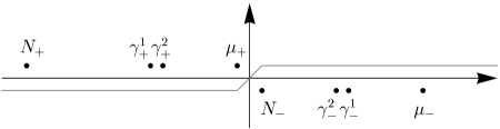
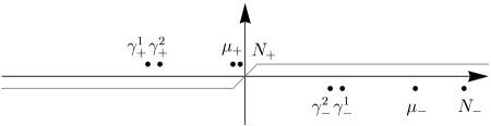
Figure 3: Poles for the unsubtracted two-photon exchange diagrams (see Fig. 2). The upper plot is for the ladder diagrams (right graphs in Fig. 2), while the lower one is for the cross diagrams (left graphs). For muonic hydrogen with $\kappa\sim 1$ the pole structure for free diagrams and for eVP contributions (see Fig. 2 a and b, respectively) is similar. Here, $N$ stands for nuclear poles, $\gamma$ is for photonic poles and $\mu$ is for muonic poles.

Once such a pole is subtracted, we see that the one-photon contribution is the only contribution for $(Z\alpha)^{2}m$ terms in all orders of $m/M$ as well as the non-recoil part of the $(Z\alpha)^{4}m$ contribution. However, a recoil part of the $(Z\alpha)^{4}m$ term arises in different gauges in different ways. The situation for the eVP (see Fig 2b) is quite similar and the pole structure is also similar.

Because of this similarity we briefly recall the situation with the $(Z\alpha)^{4}m$ terms (in all orders in $m/M$) in different gauges.

The electromagnetic interaction of two particles in different gauges is determined by the shape of the photon propagator $D_{\mu\nu}(k)$. The term $(Z\alpha)^{2}m$ originates from the $D_{00}(k)$ component, while $(Z\alpha)^{4}m$ corrections come from all components of $D_{\mu\nu}(k)$.

One can immediately see that in any covariant gauge (in contrast to the Coulomb gauge) the $D_{00}$ component depends on the energy transfer $k_{0}$ and the retardation one-photon exchange produces a correction of order $(Z\alpha)^{4}m(m/M)^{2}$. In the case of non-zero values for the $D_{i0}$ components certain terms of order $(Z\alpha)^{4}(m^{2}/M)$ can also appear from related one-photon contributions.

The static one-photon contribution obviously differs in different gauges and, after taking into account the retardation terms, the one-photon contributions still differ. One should take into account the two-photon diagrams to obtain complete $(Z\alpha)^{4}(m^{2}/M)$ and $(Z\alpha)^{4}m(m/M)^{2}$ contributions, which are indeed gauge invariant.

It is easy to estimate a ‘nominal’ order of a two-photon diagram suggesting that it converges if we neglect all the atomic effects. The order is $(Z\alpha)^{5}m^{2}/M$. To obtain a lower order in $Z\alpha$, such as $(Z\alpha)^{4}m^{2}/M$, we have to find terms divergent at low momentum.

After the heavy-pole contribution is subtracted completely, the only potentially divergent contributions are due to photon poles, if we close the contour in the lower half-plane (see Fig. 3).

The two-photon contribution in the Coulomb gauge has only a logarithmic divergence, which cannot change the fact that two-photon effects contribute in order $(Z\alpha)^{5}m^{2}/M$.

If we consider another gauge, such as the Feynman or Landau gauge, the $(Z\alpha)^{4}m^{2}/M$ terms do appear from the photonic pole contributions. We can see that such poles are important only in diagrams with $D_{00}$ components for both photons, or with $D_{i0}(q)$ contributions.

In the Coulomb gauge $D_{i0}=0$ and the $D_{00}$ component of the photon propagator does not produce a pole and technically that is why the two-photon exchange in the Coulomb gauge does not produce any $(Z\alpha)^{4}(m^{2}/M)$ and $(Z\alpha)^{4}m(m/M)^{2}$ contributions.

Once the heavy-particle pole is subtracted, the one-photon contribution is the only contribution for the $(Z\alpha)^{4}m$ terms in all orders of $m/M$ in the Coulomb gauge.

III eVP-corrected photon propagator in various gauges

Taking into account the transverse structure of the photon self-energy caused by the vacuum polarization tensor

$${\cal P}_{\mu\nu}(k)=\left(g_{\mu\nu}-\frac{k_{\mu}k_{\nu}}{k^{2}}\right)\,{\cal P}(k^{2})\;,$$ (7)

one can derive in the Landau gauge

$$D_{\mu\nu}^{\rm LeVP}(k)=\frac{1}{k^{2}}\left[g_{\mu\nu}-\frac{k_{\mu}k_{\nu}}{k^{2}}\right]\left[1+\frac{{\cal P}(k^{2})}{k^{2}}\right]\;,$$ (8)

or

$$D_{\mu\nu}^{\rm eVP}(k)=\frac{g_{\mu\nu}}{k^{2}}\left[1+\frac{{\cal P}(k^{2})}{k^{2}}\right]\;,$$ (9)

which differs only by longitudinal terms resulting from an obvious gauge transformation.

Here, for the eVP we apply Schwinger’s parametrization

$${\cal P}(k^{2})=\frac{\alpha}{\pi}\,\int_{0}^{1}{dv}\rho_{e}(v)\frac{k^{4}}{k^{2}-\lambda^{2}}\;,$$ (10)

where

$$\rho_{e}(v) = \frac{v^{2}(1-v^{2}/3)}{1-v^{2}}$$ (11)

$$\lambda^{2} = \frac{4m_{e}^{2}}{1-v^{2}}\;.$$ (12)

Indeed, neither the Landau nor Feynman gauge is well-suited for the bound-state calculations and it is helpful first to perform a gauge transformation on the photon propagator (9) to reach a more suitable gauge.

The photon propagator with an eVP correction in an arbitrary gauge can be presented in the form

$$D_{\mu\nu}(k)=D_{\mu\nu}^{\rm eVP}(k)+\chi_{\mu}k_{\nu}+k_{\mu}\chi_{\nu},$$ (13)

where $\chi=\chi(k)$ is an arbitrary function of $k$.

We expect that in recent calculations pachucki1 ; borie ; jentschura of the relativistic recoil corrections to eVP different gauges were used. In this paper we consider two choices of the gauge function $\chi(k)$ and two gauges.

The gauge function can be presented as an expansion in powers of $\alpha$

$$\chi=\chi^{(0)}+\frac{\alpha}{\pi}\chi^{(1)}\;.$$ (14)

For the $\chi^{(0)}$ we chose the transformation which is to produce the Coulomb gauge (for the free propagator), while for $\chi^{(1)}$ we consider two options, which are presented below.

The first choice is

$$\chi^{(1)}_{0} = -\int_{0}^{1}{dv}\rho_{e}\frac{k_{0}}{2(k^{2}-\lambda^{2})({\bf k}^{2}+\lambda^{2})}\;,$$

$$\chi^{(1)}_{i} = \int_{0}^{1}{dv}\rho_{e}\frac{k_{i}}{2(k^{2}-\lambda^{2})({\bf k}^{2}+\lambda^{2})}\;,$$

$$D_{00} = -\frac{\alpha}{\pi}\int_{0}^{1}{dv}\rho_{e}\frac{1}{{\bf k}^{2}+\lambda^{2}}\;,$$

$$D_{i0} = 0\;,$$

$$D_{ij} = -\frac{\alpha}{\pi}\,\int_{0}^{1}{dv}\rho_{e}\frac{1}{k^{2}-\lambda^{2}}$$ (15)

$$\times\left(\delta_{ij}-\frac{k_{i}k_{j}}{({\bf k}^{2}+\lambda^{2})}\right)\;.$$

Let us refer to it as the C1eVP gauge.

A second possibility we consider here is

$$\chi^{(1)}_{0} = -\int_{0}^{1}{dv}\rho_{e}\frac{k_{0}}{2(k^{2}-\lambda^{2}){\bf k^{2}}}\;,$$

$$\chi^{(1)}_{i} = \int_{0}^{1}{dv}\rho_{e}\frac{k_{i}}{2(k^{2}-\lambda^{2}){\bf k^{2}}}\;,$$

$$D_{00} = -\frac{\alpha}{\pi}\,\int_{0}^{1}{dv}\rho_{e}\frac{1}{k^{2}-\lambda^{2}}\,\frac{k^{2}}{{\bf k^{2}}}\;,$$

$$D_{i0} = 0\;,$$

$$D_{ij} = -\frac{\alpha}{\pi}\,\int_{0}^{1}{dv}\rho_{e}\frac{1}{k^{2}-\lambda^{2}}$$ (16)

$$\times\left(\delta_{ij}-\frac{k_{i}k_{j}}{{\bf k^{2}}}\right)\;.$$

We refer to it as the C2eVP gauge.

In the static regime (i.e., $k_{0}=0$) the choice in Eqs. (III) reproduces the potential applied in pachucki1 ; jentschura , while the choice in Eqs. (III) leads to a potential considered in borie .

We note that the gauge (III) is similar to the Coulomb gauge in a sense that the $D_{00}$ has no dependence on $k_{0}$ and there is no $D_{i0}$ component. That means that the static one-photon contribution should produce a complete result. There are two contradictory results for the $2p-2s$ Lamb splitting in literature pachucki1 ; jentschura and we confirm the latter result. Our result for muonic hydrogen is

$$\Delta E_{\rm eVP}(2p_{1/2}-2s_{1/2})=0.0187589\ {\rm meV}\,.$$ (17)

Considering the gauge (III) we note that, while $D_{i0}=0$, the $D_{00}$ component of the propagator depends on $k_{0}$ through the eVP tensor in Eq. (10) and one not only has to check the static one-photon term, but also calculate the one-photon retardation part and examine the photonic pole contributions for the two-photon diagrams (see Fig. 2b).

To check the consistency of the result obtained and to compare with other existing calculations, we perform below four separate calculations applying either a C1eVP gauge or C2eVP gauge within either the Breit-type or Grotch-type approach.

IV Calculation in the C1eVP gauge (III)

Now, let us perform the calculations in the C1eVP gauge (III), which because of lack of retardation and two-photon contributions in order $\alpha(Z\alpha)^{4}m$ (in all orders in $(Z\alpha)$) should produce a correct result in an easier way.

IV.1 Breit-type calculation

We start with a Breit-type calculations.

First, we note that as it is well known (see, e.g., breit1 ) the energy of hydrogenic levels without eVP can be found by considering a non-relativistic Schrödinger-type equation with a Hamiltonian

$$H = H_{0}+H_{1}\;,$$

$$H_{0} = \frac{{\bf p}^{2}}{2m_{R}}+V_{C}=\frac{{\bf p}^{2}}{2m_{R}}-\frac{Z\alpha}{r}\;,$$

$$H_{1} = -\frac{{\bf p}^{4}}{8}\left(\frac{1}{m^{3}}+\frac{1}{M^{3}}\right)+\frac{Z\alpha\pi}{2}\left(\frac{1}{m^{2}}+\frac{1}{M^{2}}\right)\delta^{3}(r)$$ (18)

$$- \frac{Z\alpha}{2mM\,r}\left({\bf p}^{2}+\frac{({\bf r}\cdot({\bf r}\cdot{\bf p}){\bf p})}{r^{2}}\right)$$

$$+ \frac{Z\alpha}{r^{3}}\left(\frac{1}{4m^{2}}+\frac{1}{2mM}\right)(\mbox{\boldmath$\sigma$}\cdot[{\bf r}\times{\bf p}])\;.$$

Here and in further considerations we ignore the nuclear spin terms, assuming that the results are for the center of gravity of the related hyperfine multiplet.

The result is obtained in the Coulomb gauge which is consistent with both C1eVP and C2eVP gauge we are to consider. Here the first term is responsible for the $(Z\alpha)^{2}m$ terms and the second produces $(Z\alpha)^{4}m$ contributions (in all orders in $m/M$). To find the former one has to solve the related Schrödinger equation (let us denote the energy and wave functions as $E_{0}$ and $\Psi_{0}$) and to find the latter one has to find a matrix element of $H_{1}$ over the Schrödinger-equation wave functions $\Psi_{0}$.

Applying the C1eVP gauge we find the additional terms in momentum space which are necessary to take into account eVP effects

$$H^{\rm eVP} = H_{0}^{\rm eVP}+H_{1}^{\rm eVP}\;,$$

$$H^{\rm eVP}_{0} = V_{U}({\bf k})=-4\alpha(Z\alpha)\int\limits_{0}^{1}dv\,\rho_{e}\frac{1}{{\bf k}^{2}+\lambda^{2}}\;,$$

$$H_{1}^{\rm eVP} = -4\alpha(Z\alpha)\int\limits_{0}^{1}dv\,\rho_{e}\frac{1}{{\bf k}^{2}+\lambda^{2}}$$ (19)

$$\times \Biggl{\{}\left(-\frac{{\bf k}^{2}}{2}+i\mbox{\boldmath$\sigma$}\cdot[{\bf p}_{i}\times{\bf p}_{f}]\right)\left(\frac{1}{4m^{2}}+\frac{1}{4M^{2}}\right)$$

$$+ \frac{1}{4Mm}\Biggl{(}({\bf p}_{i}+{\bf p}_{f})\cdot\left(i[\mbox{\boldmath$\sigma$}\times{\bf k}]+{\bf p}_{i}+{\bf k}_{f}\right)$$

$$\qquad\qquad\qquad\qquad-\frac{\left({\bf p}_{i}^{2}-{\bf p}_{f}^{2}\right)^{2}}{({\bf k}^{2}+\lambda^{2})}\Biggr{)}\Biggr{\}}\;.$$

The related expressions in coordinate space are

$$H^{\rm eVP}_{0} = V_{U}(r)=-\frac{\alpha}{\pi}(Z\alpha)\int\limits_{0}^{1}dv\,\rho_{e}\frac{e^{-rs_{e}}}{r}\;,$$

$$H^{\rm eVP}_{1} = \left(\frac{1}{8m^{2}}+\frac{1}{8M^{2}}\right)\nabla^{2}V_{U}$$ (20)

$$+ \left(\frac{1}{4m^{2}}+\frac{1}{2mM}\right)\frac{V_{U}^{\prime}}{r}{\bf L}\cdot{\mbox{\boldmath$\sigma$}}$$

$$+ \frac{1}{2mM}\nabla^{2}\left[V_{U}-\frac{1}{4}(rV_{U})^{\prime}\right]$$

$$+ \frac{1}{2mM}\biggl{[}\frac{V_{U}^{\prime}}{r}L^{2}+\frac{{\bf p}^{2}}{2}(V_{U}-rV_{U}^{\prime})$$

$$\phantom{\frac{1}{2mM}\biggl{[}}+(V_{U}-rV_{U}^{\prime})\frac{{\bf p}^{2}}{2}\biggr{]}\;.$$

The Hamiltonian $H^{\rm eVP}$ completely agrees with the one appearing in pachucki1 .

Again, the first term is responsible for the $\alpha(Z\alpha)^{2}m$ terms and the second one produces $\alpha(Z\alpha)^{4}m$ contributions (in all orders in $m/M$). However, now the procedure is somewhat different. We are interested only in the first order in $\alpha$ results and thus we can consider both $H^{\rm eVP}_{0}$ and $H^{\rm eVP}_{1}$ as perturbations.

To find the leading non-relativistic terms (see (1)), we have to calculate $\langle\Psi_{0}|H^{\rm eVP}_{0}|\Psi_{0}\rangle$, however, a similar contribution of higher order, $\langle\Psi_{0}|H^{\rm eVP}_{1}|\Psi_{0}\rangle$, gives only a part of the $\alpha(Z\alpha)^{4}m$ result. The other part results from second-order perturbation theory on the Schrödinger equation and it is of the form (see, e.g., pachucki1 )

$$2\langle\Psi_{0}|H^{\rm eVP}_{0}\frac{1}{\left(E-H_{0}\right)^{\prime}}H_{1}|\Psi_{0}\rangle\;,$$ (21)

where the reduced Green function $\frac{1}{\left(E-H_{0}\right)^{\prime}}$ is applied. In our calculations for the non-relativistic reduced Coulomb Green function we used its presentation in terms of smaller and larger radii (cf. pachucki2 ).

The wave function $\Psi_{0}$ is expressed in terms of the reduced mass $m_{R}$ while the dependence on $m$ and $M$ is due to apparent factors in Eqs. (18) and (IV.1) which allows to express results of our calculation of various matrix elements in terms of $C_{0}$, $C_{1}$ and $C_{2}$ as defined in Eq. (4). That is helpful for further comparison with other calculations.

Indeed, the $C_{0}$ results reproduce the values (II), as they should, while for other coefficients we find

$$C_{1}(1s) = 0.18153\dots\;,$$

$$C_{1}(2s) = 0.038089\dots\;,$$

$$C_{1}(2p_{1/2}) = 0.00090127\dots\;,$$

$$C_{1}(2p_{3/2}) = 0.00090127\dots$$ (22)

and

$$C_{2}(1s) = -0.3631\dots\;,$$

$$C_{2}(2s) = -0.07618\dots\;,$$

$$C_{2}(2p_{1/2}) = 0.003542\dots\;,$$

$$C_{2}(2p_{3/2}) = -0.004475\dots\;.$$ (23)

As we mentioned, the result for $\Delta E_{\rm eVP}(2p_{1/2}-2s_{1/2})$ is consistent with the result of jentschura .

IV.2 Grotch-type calculation

The Grotch type of approach includes a few operations (see grotch for more detail). First, we have to present the two-body wave function as a product of a free-spinor for the nucleus and a four-component muon wave function. The potential is averaged over the nuclear spinor.

The approach allows to reproduce the Dirac equation (with the reduced mass) and obtain the leading recoil correction in order $m/M$. After we neglect terms of higher order in $m/M$, we arrive at an equation

$$K\psi_{0}=E\psi_{0}\,,$$ (24)

where

$$K = \mbox{\boldmath$\alpha$}\cdot{\mathbf{p}}+\beta m+\frac{\mathbf{p}^{2}}{2M}+V$$

$$+\frac{1}{2M}\left\{\mbox{\boldmath$\alpha$}\cdot{\mathbf{p}},V\right\}+\frac{1}{4M}\left[\mbox{\boldmath$\alpha$}\cdot{\mathbf{p}},[\mathbf{p}^{2},W]\right]\,,$$

and

$$W({\bf q})=-\frac{2V({\bf q})}{{\bf q}^{2}}\;.$$

To find a solution it is helpful, following grotch , to introduce an auxiliary Hamiltonian

$$K_{1}=\mbox{\boldmath$\alpha$}\cdot{\mathbf{p}}+\beta m+V\frac{1-\beta m/M}{1-(m/M)^{2}}\,.$$ (26)

we note that

$$K=K_{0}+\Delta K+{\cal O}\left(\frac{m^{3}}{M^{2}}(Z\alpha)^{4}\right)\,,$$ (27)

where

$$K_{0}=K_{1}+\frac{K_{1}^{2}-m^{2}}{2M}+\frac{1}{4M}[K_{1},[\mathbf{p}^{2},W]]\,,$$ (28)

and

$$\Delta K=-\frac{V^{2}}{2M}-\frac{1}{4M}[V,[\mathbf{p}^{2},W]]\;.$$ (29)

As it is known grotch for the case of pure Coulomb potential, $\Delta K=0$. Let us for the moment neglect $\Delta K$ for an arbitrary potential and look for a wave function of the form

$$\psi_{0}=N\,\left(1-\frac{1}{4M}[\mathbf{p}^{2},W]\right)(1+\beta\mu)\widetilde{\psi}\,.$$ (30)

Since the Grotch-type approach does not control the $(m/M)^{2}$ terms, below we expand in $m/M$ and neglect higher-order terms everywhere where it is possible. The results of such an expansion are denoted with ‘$\simeq$’.

In particular, we find for the normalization constant $N$

$$N=\frac{1}{\sqrt{1+2\mu\,\widetilde{E}/\widetilde{m}+\mu^{2}}}\simeq 1-\frac{\widetilde{E}}{2M}\,,$$

where the involved parameters are defined below.

The final Grotch-type equation takes the form of an effective Dirac equation

$$\left(\mbox{\boldmath$\alpha$}\cdot{\mathbf{p}}+\beta\widetilde{m}+\widetilde{V}\right)\widetilde{\psi}\simeq\widetilde{E}\widetilde{\psi}\,,$$ (31)

$$\widetilde{V}=\frac{V}{\sqrt{1-\frac{m^{2}}{M^{2}}}}\simeq V\,.$$ (32)

Solutions of the Dirac equation (31), $\widetilde{\psi}$ and $\widetilde{E}$, can be found, since the final equation takes form of a Dirac equation with potential $V$ and various effective parameters. The identities for $\widetilde{\psi}$ and $\widetilde{E}$ are of the same functional form as for a solution of a Dirac equation, but they express the wave functions and energy in terms of effective parameters defined as

$$\mu = \frac{M}{m}\left(1-\sqrt{1-\frac{m^{2}}{M^{2}}}\right)\simeq\frac{m}{2M}\,,$$

$$E_{0} = E_{1}+\frac{E_{1}^{2}-m^{2}}{2M}\,,$$

$$\widetilde{E} = \frac{E_{1}-m^{2}/M}{\sqrt{1-m^{2}/M^{2}}}\simeq E_{1}-m^{2}/M\,,$$

$$\widetilde{m} = \frac{m\left(1-\frac{E_{1}}{M}\right)}{\sqrt{1-\frac{m^{2}}{M^{2}}}}\simeq m\left(1-\frac{E_{1}}{M}\right)\,,$$ (33)

One can solve the equation (31) as far as the solution of the conventional Dirac equation is known for a potential $V$ with an appropriate accuracy.

The final energy has a correction due to $\Delta K$, which was neglected in order to obtain a solvable equation. The final result for the energy is

$$E\simeq E_{0}+\langle\psi_{0}|\Delta K|\psi_{0}\rangle\,.$$ (34)

We remind that $\Delta K\propto m/M$ and here we neglect all $(m/M)^{2}$ corrections.

Now, one can introduce the potential. In the C2eVP gauge, because the photon propagator is proportional to the free propagator in the Coulomb gauge, the equation would take the same form as for the Coulomb potential, but now with potential.

$$V=V_{C}+V_{U}\,.$$ (35)

However, in the case of the C1eVP gauge, we have to introduce a certain correction, namely by redefining $W$,

$$V = V_{C}+V_{U}\,,$$

$$W = W_{C}+W_{U}\,,$$

$$W_{C} = -\frac{2V_{C}(q)}{q^{2}}\,,$$

$$W_{U} = 8\alpha(Z\alpha)\int_{0}^{1}dv\,\frac{\rho_{e}(v)}{(q^{2}+\lambda^{2})^{2}}\;.$$ (36)

In both cases, we have to solve an effective Dirac equation (IV.2) with a potential (35). The energy levels for such a Dirac equation (with a reduced mass for the particle) with $V=V_{C}$ are well known

$$E_{\rm Coul}(nlj)=m+E^{\rm(NR)}_{\rm Coul}+E_{\rm Coul}^{(0)}$$

$$\approx m-\frac{(Z\alpha)^{2}m_{R}}{2n^{2}}+\frac{(Z\alpha)^{4}m_{R}}{2n^{3}}\left(\frac{3}{4n}-\frac{1}{j+1/2}\right)$$ (37)

and the linear in $\alpha$ correction due to eVP was calculated for the Dirac wave functions as explained in Sect. II (see for details Eqs. (1), (4) and (II))

$$E_{\rm VP}=E^{(\rm NR)}_{\rm VP}+E^{(0)}_{\rm VP}\;.$$ (38)

Solving the above equations, one can arrive at (see elsewhere for details)

$$E_{0} \simeq E_{\rm Coul}(nlj)+E_{\rm VP}$$ (39)

$$- \frac{E^{\rm(NR)}_{\rm Coul}}{M}\left[E_{\rm VP}^{\rm(NR)}+\kappa\frac{\partial}{\partial\kappa}E_{\rm VP}^{\rm(NR)}\right]\,.$$

We can now return to the $\Delta K$ term. The related correction in the first order in eVP is a matrix element of

$$\Delta K \simeq -\frac{1}{2M}\biggl{(}2V_{U}V_{C}+\frac{1}{2}[V_{C},[\mathbf{p}^{2},W_{U}]]$$ (40)

$$+\frac{1}{2}[V_{U},[\mathbf{p}^{2},W_{C}]]\biggr{)}\,.$$

After a simple estimation of the operator, we find that it is sufficient to calculate the matrix element using Schrödinger-Coulomb wave functions, which are indeed well known.

More detail on the application of the Grotch-type approach to the eVP contribution will be published elsewhere elsewhere .

Finally, we obtain the results

$$C_{1}(1s) = 0.18153\dots\;,$$

$$C_{1}(2s) = 0.038087\dots\;,$$

$$C_{1}(2p_{1/2}) = 0.00090127\dots\;,$$

$$C_{1}(2p_{3/2}) = 0.00090127\dots\;,$$ (41)

which completely agree with the results (IV.1) of the Breit-type calculation.

V Calculation in the C2eVP gauge (III)

For the C2eVP gauge (III) we note that we have to calculate a static one-photon exchange, retardation one-photon contribution and two-photon contribution. Here, we first calculate the static one-photon contribution applying the Breit-type and Grotch-type techniques and afterwards we find the retardation one-photon contribution and two-photon contribution as a perturbation.

V.1 Static one-photon exchange

V.1.1 Breit-type calculation

The Breit-type Hamiltonian is somewhat different from Eq. (IV.1) and the addition is

$$\frac{\alpha(Z\alpha)}{Mm}\int\limits_{0}^{1}dv\,\rho_{e}\frac{\lambda^{2}\left({\bf p}_{i}^{2}-{\bf p}_{f}^{2}\right)^{2}}{{\bf k}^{2}({\bf k}^{2}+\lambda^{2})^{2}}$$ (42)

which shifts the results for the static contribution.

We find for the static one-photon contribution

$$C_{1}(1s) = 0.3981\dots\;,$$

$$C_{1}(2s) = 0.06357\dots\;,$$

$$C_{1}(2p_{1/2}) = 0.002845\dots\;,$$

$$C_{1}(2p_{3/2}) = 0.002845\dots\;,$$ (43)

and

$$C_{2}(1s) = -0.7961\dots\;,$$

$$C_{2}(2s) = -0.1271\dots\;,$$

$$C_{2}(2p_{1/2}) = -0.0003444\dots\;,$$

$$C_{2}(2p_{3/2}) = -0.008362\dots\;,$$ (44)

which indeed does not coincide with Eqs. (IV.1) and (IV.1), because such a contribution is not gauge invariant.

V.1.2 Grotch-type calculation

A similar correction should be introduced into the Grotch-type approach. As we already mentioned, since the C2eVP gauge is proportional to the Coulomb gauge, we can use the same kind of equation as for the Coulomb gauge with a potential

$$V=V_{C}+V_{U}$$

and the $W$ function defined within the same functional relation as for the Coulomb potential, namely as

$$W(q)=-\frac{2V(q)}{q^{2}}\;.$$

The effective Dirac equation, which does not involve $W$, is indeed the same as in C1eVP gauge, while the $\Delta K$ correction proportional to $W$ is different.

Proceeding similarly to described in Sect. IV.2 we arrive at

$$C_{1}(1s) = 0.39818\dots\;,$$

$$C_{1}(2s) = 0.063585\dots\;,$$

$$C_{1}(2p_{1/2}) = 0.0028496\dots\;,$$

$$C_{1}(2p_{3/2}) = 0.0028496\dots\;,$$ (45)

which is consistent with Eq. (V.1.1) and somewhat disagrees with borie .

In particular, our result for $E_{\rm VP}^{\rm(rel)}-E_{\rm VP}^{(0)}$ for the $2p-2s$ splitting for the static contribution is $-0.0042785$ meV which is to be compared with $-0.0041$ meV in borie .

The relativistic recoil eVP correction in light muonic atoms was calculated by Borie in borie in a way somewhat different from, but consistent with our treatment here of the Grotch-type approach in the gauge C2eVP.

In the recent paper borie some minor corrections to the earlier papers borie82 and borie05 were introduced. Still, we failed to reproduce exactly the numerical results borie for the correction neither by expressions given in borie nor by those presented in borie82 , where further details of the calculation were given. Apparently, expressions of borie still contain misprints.

What is more important, the results we obtained in this section also disagree with the result borie . The departure grows systematically between muonic hydrogen, deuterium and helium. (The results for the latter are presented in Sect. VII of our paper.)

Meanwhile, we have discovered that our expression for the energy correction agrees with one presented in borie82 (see Eq. (116); it is also reproduced in Appendix A of borie ). Our numerical results can be reproduced if we modify the erroneous expression for the term $\left\langle\frac{Z\alpha}{3r^{4}}Q_{4}\right\rangle$ presented in Appendix A of borie .

Thus, we conclude that the result borie for the relativistic recoil correction in light muonic atoms is unfortunately both incomplete because of lack of two-photon contributions and incorrect (because even the partial calculation contains a numerical error).

V.2 Retardation one-photon exchange

The retardation one-photon contribution and an essential two-photon contribution can be calculated directly as a perturbation, since they are already related to effective potentials which are smaller by a factor $(Z\alpha)^{2}$ than the non-relativistic contributions. It is also important that the second order perturbation term (see (21)) is the same as in C1eVP gauge. That is because the free term of eVP propagator is the same for both gauges (which determines $H_{1}$) and the static limit of the eVP term of the propagator also does not change (which determines $H_{0}^{\rm eVP}$). That says that only first-order perturbation theory terms are essential, otherwise the second-order terms similar to (21) would appear.

One can immediately find a related effective addition to the Hamiltonian due to retardation

$$\frac{\alpha(Z\alpha)}{M^{2}}\int\limits_{0}^{1}dv\,\rho_{e}\frac{\lambda^{2}\left({\bf p}_{i}^{2}-{\bf p}_{f}^{2}\right)^{2}}{{\bf k}^{2}({\bf k}^{2}+\lambda^{2})^{2}}$$ (46)

or in coordinate space

$$H_{\rm retard} = \frac{\alpha(Z\alpha)}{4\pi\,M^{2}}\int_{0}^{1}dv\rho(v)$$

$$\times \left[\left\{{\bf p}^{4},Q(r)\right\}-2{\bf p}^{2}Q(r)\,{\bf p}^{2}\right]\,,$$

where

$$Q(r)=\frac{1}{\lambda^{2}r}-(2+rs_{e})\frac{e^{-rs_{e}}}{2\lambda^{2}r}\,.$$ (48)

The results of direct calculations of $C_{1}$ and $C_{2}$ in muonic hydrogen are compiled in Tables 1 and 2, respectively. The retardation effects under consideration are of order $\alpha(Z\alpha)^{4}m(m/M)^{2}$ and contribute only to $C_{2}$.

Contribution	$C_{1}(1s)$	$C_{1}(2s)$	$C_{1}(2p_{1/2})$	$C_{1}(2p_{3/2})$
Static	$\phantom{-}0.39818$	$\phantom{-}0.063585$	$\phantom{-}0.0028496$	$\phantom{-}0.0028496$
Retardation	$\phantom{-}0\phantom{.00000}$	$\phantom{-}0\phantom{.000000}$	$\phantom{-}0\phantom{.0000000}$	$\phantom{-}0\phantom{.0000000}$
Two-photon	$-0.21654$	$-0.025483$	$-0.0019484$	$-0.0019484$
Total	$\phantom{-}0.18164$	$\phantom{-}0.038102$	$\phantom{-}0.0009012$	$\phantom{-}0.0009012$

Table 1: $C_{1}$ coefficients in the C2eVP gauge.

Contribution	$C_{2}(1s)$	$C_{2}(2s)$	$C_{2}(2p_{1/2})$	$C_{2}(2p_{3/2})$
Static	$-0.7961$	$-0.1271\phantom{0}$	$-0.0003444$	$-0.008362$
Retardation	$\phantom{-}0.2165$	$\phantom{-}0.02548$	$\phantom{-}0.001948\phantom{0}$	$\phantom{-}0.001948$
Two-photon	$\phantom{-}0.2165$	$\phantom{-}0.02548$	$\phantom{-}0.001948\phantom{0}$	$\phantom{-}0.001948$
Total	$-0.3631$	$-0.07618$	$\phantom{-}0.003552\phantom{0}$	$-0.004465$

Table 2: $C_{2}$ coefficients in the C2eVP gauge.

V.3 Two-photon exchange

For the two-photon exchange we have performed a calculation of the photon pole contributions. One has to carefully consider splitting of the contributions. We are interested in those which are singular at low momentum. Actually the photon-pole contribution is divergent in a formal sense at high momentum, but such a divergence is in order $\alpha(Z\alpha)^{5}m^{2}/M$ and thus is of a higher order. One has to separate properly the low-momentum and high-momentum contributions, and after that only the low-momentum one is of interest. The results are summarized in Tables 1 and 2, respectively.

We note that the sum of the results in the C2eVP gauge produces a result consistent with those in the C1eVP gauge. We may also find an effective potential induced by a low-momentum contribution of the two-photon kernel. It is of the form

$$- \frac{\alpha(Z\alpha)^{2}}{2\pi M}\int\frac{d^{3}{\bf q}}{(2\pi)^{3}}\int\limits_{0}^{1}dv\,\rho_{e}\frac{\lambda^{2}}{({\bf q}^{2}+\lambda^{2})^{2}}$$ (49)

$$\times \frac{4\pi}{{\bf q}^{2}}\frac{4\pi}{({\bf k}-{\bf q})^{2}}\left({\bf q}^{2}-{\bf k}\cdot{\bf q}\right)\,.$$

For the diagonal matrix elements we can replace the expression (49) by an effective potential of the form

$$-\frac{\alpha(Z\alpha)}{Mm_{R}}\int\limits_{0}^{1}dv\,\rho_{e}\lambda^{2}\frac{\left({\bf p}_{i}^{2}-{\bf p}_{f}^{2}\right)^{2}}{{\bf k}^{2}({\bf k}^{2}+\lambda^{2})^{2}}\,.$$ (50)

We see that at the end of the day the final effective Hamiltonians in both gauges are the same. The addition in the C2eVP gauge (42) for the static term is eventually cancelled out by the retardation (46) and two-photon (50) terms:

$$0 = \alpha(Z\alpha)\int\limits_{0}^{1}dv\,\rho_{e}\frac{\lambda^{2}\left({\bf p}_{i}^{2}-{\bf p}_{f}^{2}\right)^{2}}{{\bf k}^{2}({\bf k}^{2}+\lambda^{2})^{2}}$$ (51)

$$\times \left(\frac{1}{Mm}+\frac{1}{M^{2}}-\frac{1}{Mm_{R}}\right)\,.$$

VI Finite-nuclear-size corrections

As we mentioned in the introduction, the definition of the nuclear radius for different spin values can produce additional corrections in order $(Z\alpha)^{4}m(m/M)^{2}$ and $\alpha(Z\alpha)^{4}m(m/M)^{2}$. For this reason we consider in this paper the finite-nuclear-size (FNS) corrections. While the relation between the eVP recoil contributions and such corrections is considered in the next section, here we revisit the FNS contributions with inclusion of eVP.

Such contributions are known for a while friarNS ; pachucki2 ; EGS , basically numerically borie05 . Here we present semi-analytic results.

We treat the FNS effects non-relativistically. In this case the FNS correction is of the form

$$\Delta E_{\rm FNS} = \frac{R^{2}_{N}}{6}\langle\Psi|\nabla^{2}(V_{C}+V_{U})|\Psi\rangle$$ (52)

$$= \Delta E_{\rm FNS}^{(0)}+\Delta E_{\rm FNS}^{(1)}+\Delta E_{\rm FNS}^{(1)}\;,$$

where the wave function is the result of the Schrödinger equation with the reduced mass and potential $V_{C}+V_{U}$ and $R_{N}$ is the rms nuclear charge radius. The result is not vanishing only for the $s$ states.

The leading term for the splitting

$$\Delta E_{\rm FNS}^{(0)}(2s)=\frac{(Z\alpha)^{4}}{12}\,(R_{N}^{2}m_{R}^{2})m_{R}$$ (53)

is applied for a determination of the nuclear size radius from the experimental Lamb shift value and it is important to calculate corrections to it.

The two corrections can be obtained in a way similar to a non-relativistic calculation of the leading eVP correction to the hyperfine structure (cf. pachucki2 ; martynenko05 ; muhfs ). The first term is

$$\Delta E_{\rm FNS}^{(1)}=\frac{2\pi Z\alpha}{3}R^{2}_{N}\left(|\Psi(0)|^{2}-|\Psi_{C}(0)|^{2}\right)\;.$$ (54)

It is convenient to present the eVP correction in the form

$$\Delta E_{\rm FNS}^{(1)}=\Delta E_{\rm FNS}^{(0)}\;\frac{|\Psi(0)|^{2}-|\Psi_{C}(0)|^{2}}{|\Psi_{C}(0)|^{2}}\;,$$ (55)

where we express the correction in terms of the leading term and the eVP correction to the wave function at the origin. The latter was studied in pi_1s ; muhfs ; soto ; vp32 .

The other term is

$$\Delta E_{\rm FNS}^{(2)}=\frac{R^{2}_{N}}{6}\langle\Psi_{C}|\nabla^{2}{V_{U}}|\Psi_{C}\rangle.$$ (56)

It was also found in pi_1s :

$$\Delta E_{\rm FNS}^{(2)}(2s)=\frac{\alpha}{\pi}\,G_{2s}(\kappa/2)\,\Delta E_{\rm FNS}^{(0)}(2s)\;,$$ (57)

where

$$G_{2s}(z) = -\frac{\pi}{3z^{3}}+\frac{24-44z^{2}-29z^{4}+22z^{6}}{36z^{2}(1-z^{2})^{2}}$$

$$+ \frac{8-20z^{2}+33z^{4}-20z^{6}+8z^{8}}{12z^{3}(1-z^{2})^{2}}\,A(z)\,,$$

where $A(z)$ is defined by Eq. (2).

The numerical results on the finite-nuclear-size corrections for the $2s$ state in light muonic atoms are summarized in Table 3. Note that for the Lamb shift the signs of the corrections are opposite. The results are slightly different but rather consistent with ones presented in borie .

Atom	$\Delta E_{\rm FNS}^{(0)}$	$\Delta E_{\rm FNS}^{(1)}$	$\Delta E_{\rm FNS}^{(2)}$	$\Delta E_{\rm FNS}$
$\mu$H	5.1975	0.0170	0.0110	5.2254
$\mu$D	6.0732	0.0205	0.0132	6.1069
$\mu^{3}$He	102.52	0.5200	0.3230	103.37
$\mu^{4}$He	105.32	0.5360	0.3330	106.19

Table 3: The non-relativistic finite-nuclear-size corrections for the $2s$ state in light muonic atoms (in meV$\cdot\,(R_{N}/{\rm fm})^{2}$). Here, $\mu$He stands for muonic helium ions.

VII Results for the Lamb shift in light muonic atoms

To conclude a calculation of the relativistic recoil corrections, we have to fix the definition of the nuclear charge radius, which varies in literature. That is important for the relativistic recoil corrections because with different definitions of the nuclear charge radius a certain part of the $(Z\alpha)^{4}(m/M)^{2}m$ and $\alpha(Z\alpha)^{4}(m/M)^{2}m$ terms may be incorporated in the nuclear-finite-size term.

The nuclear spin takes different values for light muonic atoms, namely, $I=1/2$ for a muonic hydrogen and muonic helium-3 ion, $I=0$ for a muonic helium-4 ion and $I=1$ for muonic deuterium. The different nuclear spin values are related to different effective two-body Breit-type equations for structureless particles (see, e.g., scalar ; vector ).

To be consistent with the experimental determination, we use the same definitions of the nuclear charge radius as applied in scalar ; vector ; vector1 ; friar ; codata ; nature .

In this convention the Zitterbewegung term is present for half-integer spin nuclei, and not present for the integer case.

The related calculation produces the results summarized in Table 4.

Atom	$\Delta E_{\rm eVP}(2p_{1/2}-2s_{1/2})$	$\Delta E_{\rm eVP}(2p_{3/2}-2p_{1/2})$
$\mu$H	0.018759	0.0049638
$\mu$D	0.021781	0.0057361
$\mu^{3}$He	0.509340	0.2692000
$\mu^{4}$He	0.521100	0.2750200

Table 4: Relativistic recoil corrections to the Lamb shift and fine structure in light muonic atoms (in meV).

Our results for the Lamb shift in light muonic atoms agree with the results of jentschura and disagree with the results of borie and martynenko07 .

For the fine structure, the results are also presented in Table 4.

The result has been obtained in the C1eVP gauge within Breit-type calculations and to control them we also performed a Grotch-type calculation in the same gauge. They are in perfect agreement with each other.

VIII Summary

Concluding, relativistic recoil contributions in orders $\alpha(Z\alpha)^{4}m(m/M)$ and $\alpha(Z\alpha)^{4}m(m/M)^{2}$ to the Lamb shift in muonic hydrogen were revisited. The results published previously by various authors and obtained by different methods are inconsistent. In particular, result of the Breit-type calculation in jentschura is twice smaller than the related result from the Grotch-type evaluation in borie . The value of discrepancy, 0.002 meV, is comparable with the experimental uncertainty of 0.003 meV nature .

We perform here an evaluation in both approaches and find that the discrepancy between jentschura and borie is caused by the fact that both calculated the same value, namely the static one-photon exchange, which is not gauge invariant. They applied different gauges. The gauge invariant value is a sum of the static term and two other contributions, which are the retardation correction and two-photon contribution. While they are absent for the calculation of the $\alpha(Z\alpha)^{4}m(m/M)$ term in one gauge, they are not vanishing in the other.

Once such contributions are taken into account and a relatively small numerical error in calculation borie is fixed, we find perfect agreement between two approaches. Our results agree with those of jentschura .

We also consider other light atoms and perform calculations for the Lamb shift muonic deuterium and two isotopes of muonic helium. For a muonic helium-4 ion we agree with jentschura and disagree with martynenko07 .

For control purposes we have also performed calculations of the fine structure in order $\alpha(Z\alpha)^{4}m(m/M)$ and $\alpha(Z\alpha)^{4}m(m/M)^{2}$. The result for the latter can be completely restored from the result from Dirac equation (see, e.g., rel2 ). Our result for muonic hydrogen is in agreement with fs_martynenko .

References

- (1) R. Pohl, A. Antognini, F. Nez, Fernando D. Amaro, F. Biraben, J. M. R. Cardoso, D. S. Covita, A. Dax, S. Dhawan, L. M. P. Fernandes, A. Giesen, T. Graf, T. W. Hänsch, P. Indelicato, L. Julien, Cheng-Yang Kao, P. Knowles, E.-O. Le Bigot, Yi-Wei Liu, J. A. M. Lopes, L. Ludhova, C. M. B. Monteiro, F. Mulhauser, T. Nebel, P. Rabinowitz, J. M. F. dos Santos, L. A. Schaller, K. Schuhmann, C. Schwob, D. Taqqu, J. F. C. A. Veloso and F. Kottmann, Nature (London) 466, 213 (2010).
-
(2)
J. C. Bernauer, P. Achenbach, C. Ayerbe Gayoso, R. Böhm,
D. Bosnar, L. Debenjak, M. O. Distler, L. Doria, A. Esser,
H. Fonvieille, J. M. Friedrich, J. Friedrich, M. Gómez Rodríguez
de la Paz, M. Makek, H. Merkel, D. G. Middleton, U. Müller,
L. Nungesser, J. Pochodzalla, M. Potokar, S. Sńchez Majos,
B. S. Schlimme, S. Širca, Th. Walcher, and M. Weinriefer,
Phys. Rev. Lett. 105, 242001 (2010);
Phys. Rev. Lett. 107, 119102 (2011). - (3) P. J. Mohr, B. N. Taylor, and D. B. Newell, Rev. Mod. Phys. 80, 633 (2008).
- (4) S. G. Karshenboim, V. G. Ivanov, E. Yu. Korzinin, and V. A. Shelyuto, Phys. Rev. A 81, 060501 (2010),
- (5) S. G. Karshenboim, E. Yu. Korzinin, V. G. Ivanov and V. A. Shelyuto, Pis’ma v ZhETF 92, 9 (2010) [in Russian]; JETP Letters 92, 8 (2010).
- (6) W. A. Barker and F. N. Glover, Phys. Rev. 99, 317 (1955).
- (7) V. B. Berestetskii, E. M. Lifshitz, and L. P. Pitaevskii, Quantum electrodynamics, Pergamon, Oxford (1982).
- (8) H. Grotch and D. R. Yennie, Z. Phys. 202, 425 (1967).
- (9) A. Veitia and K. Pachucki, Phys. Rev. A 69, 042501 (2004).
- (10) E. Borie, arxiv 1103.1772v5.
- (11) U. D. Jentschura, Phys. Rev. A 84, 012505 (2011)
-
(12)
A. B. Mickelwait and H. C. Corben, Phys. Rev. 96, 1145 (1954);
G. E. Pustovalov, Zh. Eksp. Teor. Fiz. 32, 1519 (1957) [in Russian]; Sov. Phys. JETP 5, 1234 (1957);
D. D. Ivanenko and G. E. Pustovalov, Usp. Fiz. Nauk 61, 27 (1957) [in Russian]; Adv. Phys. Sci. 61, 1943 (1957). - (13) S. G. Karshenboim, V. G. Ivanov, and E. Yu. Korzinin, Eur. Phys. J. D 39, 351 (2006).
- (14) E. Borie, Zeitschrift für Physik A Hadrons and Nuclei 278, 127 (1976).
-
(15)
S. G. Karshenboim, Can. J. Phys. 76, 169 (1998);
ZhETF 116, 1575 (1999) [in Russian]; JETP 89, 850 (1999). - (16) E. Yu. Korzinin, V. G. Ivanov, and S. G. Karshenboim, Eur. Phys. J. D 41, 1 (2007).
- (17) K. Pachucki, Phys. Rev. A 53, 2092 (1996)
-
(18)
G. P. Lepage, Phys. Rev. A 16, 863 (1977);
G. T. Bodwin, D. R. Yennie, and M. A. Gregorio, Rev. Mod. Phys. 57, 723 (1985);
J. Sapirstein and D. R. Yennie, in T. Kinoshita (Ed.), Quantum Electrodynamics (World Sci., Singapore, 1990), p. 560;
M. I. Eides, S. G. Karshenboim, and V. A. Shelyuto, Ann. Physics 205, 231 (1991). - (19) V. G. Ivanov, S. G. Karshenboim, and E. Yu. Korzinin, in preparation.
- (20) E. Borie, Rev. Mod. Phys 54, 67 (1982).
- (21) E. Borie, Phys. Rev. A 71, 032508 (2005).
- (22) J. L. Friar, Zeit. f. Physik A 292, 1 (1979); Zeit. f. Physik A 303, 84 (1981).
- (23) M. I. Eides, H. Grotch, and V. A. Shelyuto, Theory of Light Hydrogenic Bound States (Springer, Berlin Heidelberg New York, 2007).
- (24) A. P. Martynenko, Phys. Rev. A 71, 022506 (2005).
- (25) S. G. Karshenboim, E. Yu. Korzinin, and V. G. Ivanov, Pis’ma v ZhETF 88, 737 (2008) [in Russian]; JETP Letters 88, 641 (2008).
- (26) S. G. Karshenboim, U. Jentschura, V. Ivanov, and G. Soff, Eur. Phys. J. D2, 209 (1998).
- (27) D. Eiras and J. Soto, Phys. Lett. 491B, 101 (2000).
- (28) V. G. Ivanov, E. Yu. Korzinin, and S. G. Karshenboim, Phys. Rev. D80, 027702 (2009).
-
(29)
D. A. Owen, Phys. Rev. D 42, 3534 (1990); D 46, 4782
(E) (1992); Found. Phys. 24, 273 (1994);
M. Halpert and D. A. Owen, J. Phys. G 20, 51 (1994). - (30) K. Pachucki and S. G. Karshenboim, J. Phys. B 28, L221 (1995).
- (31) I. B. Khriplovich, A. I. Milstein, and R. A. Sen’kov, Phys. Lett. A 221, 370 (1996); ZhETF 111, 1935 (1997) [in Russian]; JETP 84, 1054 (1997).
- (32) J. L. Friar, J. Martorell, and D. W. L. Sprung, Phys. Rev. A56, 6, 4579 (1997)
- (33) A. P. Martynenko, Phys. Rev. A 76, 012505 (2007).
- (34) A. P. Martynenko, Yad. Fiz. 71, 126 (2008) [in Russian]; Phys. At. Nucl. 71, 125 (2008).