Two dimensional Dirac fermions in the presence of long-range correlated disorder

Abstract

We consider 2D Dirac fermions in the presence of three types of disorder: random scalar potential, random gauge potential and random mass with long-range correlations decaying as a power law. Using various methods such as the self-consistent Born approximation (SCBA), renormalization group (RG), the matrix Green function formalism and bosonisation we calculate the density of states and study the full counting statistics of fermionic transport at lower energy. The SCBA and RG show that the random correlated scalar potentials generate an algebraically small energy scale below which the density of states saturates to a constant value. For correlated random gauge potential, RG and bosonisation calculations provide consistent behavior of the density of states which diverges at zero energy in an integrable way. In the case of correlated random mass disorder the RG flow has a nontrivial infrared stable fixed point leading to a universal power-law behavior of the density of states and also to universal transport properties. In contrast to uncorrelated case the correlated scalar potential and random mass disorders give rise to deviation from the pseudodiffusive transport already to lowest order in disorder strength.

I Introduction

In the recent years significant attention has been attracted by materials exhibiting two dimensional fermionic excitations with linear dispersion relation near the Fermi level. These excitations share many properties with massless relativistic particles but with a velocity reduced with respect to the speed of light. The seminal example of such material is graphene,novoselov05 the low energy properties of which are described by two dimensional (2D) gas of Dirac fermions.castroneto09 ; dassarma11 More recently, 2D Dirac fermions have also emerged as the effective low energy degree of freedom in the surface states of 3D topological insulators,fu07 ; moore07 ; roy09 such as the materials in the Bi₂Se₃ familyhsieh08 and strained HgTe.hancock11 Dirac excitations have been also found in unconventional superconductor with $d$-wave symmetryorenstein00 ; asboth11 ; wang11 ; durst00 , in the quasi-2D organic conductor $\alpha$-(BEDT-TTF)₂ I₃ under pressure,katayama06 ; kobayashi07 ; fukuyama07 ; goerbig08 ; nishine10 ; kobayashi11 and even in photonic crystals.huang11

The peculiar features of Dirac fermions lead to unfamiliar transport properties in all these materials. Of particular interest are the vanishing of the density of states at the Dirac (or neutrality) point, and the unusual scattering properties of the Dirac particles, a striking example of which being provided by the so-called Klein tunneling phenomenon: an excitation incident normal to a potential barrier crosses this barrier completely even for energies smaller than the barrier height.castroneto09 A consequence of that is the total absence of backscattering for these Dirac fermions. The peculiarities of the spectrum near the Dirac point also affect transport strongly. In undoped graphene, due to the evanescent nature of the states at the Dirac point, transport in a clean sample is similar to that in a diffusive wire.Tworzydlo06 Moreover, all the different cumulants of current fluctuations in a graphene sample behave as in a diffusive wire rather than in a ideal metallic system. In particular, pseudodiffusive conductance scales with the length of the system $L$ as $1/L$ in contrast with the $L^{0}$ scaling of ideal conducting systems. The associated Fano factor defined as the ratio between the shot noise power and the current has the same universal value $F=1/3$ as for diffusive metallic wires instead of $F=0$ for ideal conductors. Remarkably, the conductivity minimum of graphene at the neutrality point due to evanescent modes is of order $e^{2}/h$, i.e. finite despite the vanishing of the density of states. Though the conductivity minimum remains almost constant in very broad temperature range its sample-dependance indicates the importance of disorder for the transport properties of graphene.mucciolo10

Due to these specificities, numerous studies have focus on the effect of a random scattering potential on transport of Dirac states.ostrovsky06 ; khveshchenko07 ; schuessler09 ; schuessler10 Indeed, various kinds of disorder are naturally present in real materials, and affect in a dominant way the electronic transport properties. They can be of different origin: lattice defects, impurities, ripples in graphene sheet that distort locally the lattice, adatoms deposited on the surface of a graphene sample,shevtsov11 atomic steps on the surface of topological insulators, etc. Theoretical research on disordered 2D Dirac fermions was also motivated initially by its relevance to Quantum Hall transitions.ludwig94 Building on this pioneering work, recent studies have focused on the effect of the different types of disorder on the transport properties of Dirac fermions as in the limit of low energy, i.e. around the Dirac point, as well as away from half filling. In the present paper, we do not consider the highly doped weak localization regimemaccann06 ; kharitonov08 corresponding to $k_{F}l_{0}\gg 1$, where $l_{0}$ is the mean free path, and concentrate mostly on the transport near the Dirac point where $k_{F}\to 0$. It has been shown that the conductivity at half filling depends not only on the type of disorder but also on the infrared cutoff, so that it potentially can depend on the geometry of the physical setup.ostrovsky06 The role of infrared cutoff can be played by either the mean free path, the Fermi length or the size of the system. These different cases allow to identify several transport regimes.schuessler09 Fixing geometry, for example to wide-and-short rectangle with many propagating transverse modes one can compute the conductance and the Fano factor for each regime.schuessler10 Most of the previous studies addressed the case where the scattering potential is uncorrelated in space. This is the case for instance if it is originated from localized point-like scatterers distributed independently from each other. However, several physically relevant types of disorder sources exhibit long-range correlations.

For example, a graphene sheet is known to develop static shape fluctuations due to the unavoidable thermodynamic instability of 2D crystals with respect to both crumpling and bending. These ripples survive at low temperatures and can be viewed as a static random gauge potential playing the role of a quenched disorder on the electronic time scale (see below). The theory of 2D elastic membranes predicts the strength of the local height fluctuations which give rise to long-range algebraic correlation of this random gauge potential.katnelson07 ; fasolino07 ; khveshchenko07 ; abedpour07 ; guinea08 A second example, in the case of the surface states of topological insulators, is surface roughnessalpichshev11 which is one of the dominant form of disorder in these materials. A typical roughness created by atomic steps can induce a scattering potential with algebraically decaying correlations.nozieres87 ; fedorenko06 As a last example, the adsorption of magnetic adatoms on the surface of topological insulators has been proposed as a way to control the electronic properties of the surface states.abanin11 If the characteristic spin flip time of magnetic adatoms exceeds the mean free time of the electrons in the surface states these adatoms can be also viewed as a source of quenched disorder of both random gauge and random mass types. In the vicinity of the paramagnetic-ferromagnetic transition, induced by the RKKY-type surface interactions, critical magnetization fluctuations will give rise to a quenched disorder on electronic time scales with power law correlations in space.

Motivated by these physical examples, in this paper we consider the general properties of 2D Dirac fermions in the presence of various weak random potentials possessing algebraic spatial correlations. Using several analytical techniques, we consider perturbatively these disorder potentials. We focus on the effect of these long-range correlations on the density of states and also transport properties discussing the cases relevant for the three above mentioned examples. In particular, we will compute the unknown to our knowledge density of states for correlated random potential and random mass. We will show that the previous estimationkhveshchenko08 of the density of states for correlated random gauge potential is wrong. We will find the correct density of states using two different methods: renormalization group and bosonisation. We will develop a framework to study transport properties in the presence of correlated disorder using the matrix Green function formalism introduced by Nazarov.nazarov94 ; ryu07 Our approach goes beyond the previous work of Khveshchenkokhveshchenko07 ; khveshchenko08 who also considered LR correlated potentials but focused on the multi fractal spectrum of wave functions at the Dirac points and the conductance within the self consistant Born approximation (SCBA).

The paper is organized as follows. Section II introduces the model. In Sec. III we consider the SCBA approximation. In Sec. IV using the matrix Green function formalism we study the full counting statistics for a wide-and-short rectangle sample at the neutrality point. In Sec. V we derive RG equations to one-loop order and discuss the properties of the systems with different type of disorder. In Sec. VI we use bosonisation technique for systems with LR correlated random gauge potential. In Sec. VII we summarize the obtained results.

II Model

II.1 Single flavor Dirac model

Whenever they appear in a 2D or quasi-2D material, like graphene, lattice Dirac fermions are constrained by the Nielsen-Ninomiya theoremnielsen81 to appear by pair of species. Practically, this implies the existence of an even number of Dirac cones in the first Brillouin zone when considering the low energy dispersion relation. Indeed, in graphene two Dirac cones exist at the inequivalent points $K$ and $K^{\prime}=-K$ at the zone boundary. However, any potential varying on scales much larger that the atomic scale $\pi/K$ will leave the two Dirac cones uncoupled. In this case, the effect of the potential can be described by considering its effect on a single Dirac cone, treating the presence of the other Dirac point as an effective degeneracy. We thus lead to consider a single species of non-interacting massless 2D Dirac fermions in the presence of a random potential, described by the Hamiltonian

$$H=H_{0}+V(x,y),$$ (1)

where $H_{0}$ is the kinetic Hamiltonian of free Dirac fermions with the Fermi velocity $v_{0}$,

$$H_{0}=-iv_{0}(\sigma_{x}\partial_{x}+\sigma_{y}\partial_{y}),$$ (2)

and $V(x,y)$ is a random disorder potential. Here and in the following $\sigma_{0}=\mathds{1}$, $\sigma_{\mu}$, $\mu=x,y,z$ are the respective Pauli matrices, and we set $\hbar=1$ for convenience. This type of potential, without any Fourier component which couple the different Dirac species, is often denoted as a long-range potential. This notation, which refers to correlations at the scale of the lattice space, should not be confused with the long-range (LR) correlation in space on which we focus in this paper. The latter characterizes the long distance $q\simeq 0$ behavior of the random potential correlations. Note that in the case of graphene, as well as in the quasi-2D $\alpha$-(BEDT-TTF)₂ I₃, the Pauli matrices entering the relativistic kinetic Hamiltonian refer to a pseudo-spin describing the relative weight of the electronic wave function on two sub-lattices. Thus, the coupling of the random potential to these two sub lattices will be reflected in the parametrization introduced below for this potential in terms of these Pauli matrices.

The case of surface states of topological insulators is different.hasan10 ; qi11 In these materials, a strong spin orbit interaction opens a gap for bulk states. The non trivial topological order characterizing the filled bands of this insulator implies the existence of Dirac fermions surface states. Since they are not constrained by the Nielsen-Ninomiya theorem, they occur around an odd number of Dirac points in the first Brillouin zone. In the simplest topological insulators, a single Dirac cone exists at the surface of these insulators, the properties of which control the surface transport properties of the material. In this case, the relativistic kinetic Hamiltonian of the surface states contains a real magnetic term reflecting the bulk spin orbit interaction. This term should be an odd function of the electron spin, which we take for simplicity as the in plane component of the spin, obtaining effectively Eq. (1). In this case, the parametrization of disorder depends on the coupling of the corresponding potential to the spin of the electrons. In topological insulators, the bulk topological order at the origin of this odd number of Dirac species, also prevents time-reversal invariant disorder from localizing these states. This robustness property is in fact the result of an odd number of Dirac species as opposed to an even number, and will play no role in the decoupled cones treatment of disorder that we will perform.

As discussed above, we parametrize the disorder potential using the following decomposition

$$V(x,y)=\sum\limits_{\mu=0,x,y,z}\sigma_{\mu}V_{\mu}(x,y).$$ (3)

In the usual terminology of disordered graphene the term with $\mu=0$ is called random potential disorder, the terms with $\mu=x,y$ random gauge disorder and the term with $\mu=z$ random mass disorder. We will keep this terminology, even though for systems with real spin (instead of pseudo-spin) like topological insulators they may have a different physical interpretation. Fox instance, in topological insulators the terms with $\mu=x,y,z$ in Eq. (3) correspond to real random magnetic impurities on the conducting surface.

In what follows the disorder potentials $V_{\mu}(r)$ [$\mathbf{r}=\{x,y\}$] are taken to be random and Gaussian with $\langle V_{\mu}(\mathbf{r})\rangle=0$ and correlators

$$\langle V_{\mu}(\mathbf{r})V_{\nu}(\mathbf{r}^{\prime})\rangle=2\pi v_{0}^{2}\delta_{\mu\nu}g_{\mu}(\mathbf{r}-\mathbf{r}^{\prime}).$$ (4)

For the sake of convenience we fix the form of the correlator in Fourier space

$$\langle V_{\mu}(\mathbf{k})V_{\nu}(\mathbf{k}^{\prime})\rangle=(2\pi)^{3}v_{0}^{2}\delta(\mathbf{k}+\mathbf{k}^{\prime})\delta_{\mu\nu}(\alpha_{\mu}+\beta_{\mu}|\mathbf{k}|^{a-2}).$$ (5)

This form of the correlator corresponds in real space to

$$g_{\mu}(\mathbf{r})=\alpha_{\mu}\delta(\mathbf{r})+\beta_{\mu}\mathcal{A}_{a}|\mathbf{r}|^{-a},\ \ \ \mathcal{A}_{a}=\frac{2^{a}\,\Gamma(a/2)}{4\pi\Gamma(1-a/2)}$$ (6)

The exponent $a$ is determined by the nature of disorder correlations or by internal or fractal dimension of the extended defects. In the presence of extended defects of internal dimension $\varepsilon_{d}$ randomly orientated the corresponding exponent $a=2-\varepsilon_{d}$. For instance, the presence linear dislocations or atomic steps with random orientations on the surface of topological insulator ($\varepsilon_{d}=1$) leads to LR correlated disorder with $a=1$.fedorenko06 In the case of ripples of a graphene sheet, an evaluation of the correlation of the generated gauge potential provides an exponentkatnelson07 ; fasolino07 ; khveshchenko07 ; abedpour07 ; guinea08 $a\approx 1.6$. In the case of magnetic adatoms deposited at the surface of topological insulators,abanin11 the induced magnetic disorder correlations will decay as a power law with $a=\eta$ where $\eta=1/4$ is the critical exponent describing the magnetization correlation function in 2D Ising system. Hence, these examples provide strong motivation to consider the effect of these algebraic correlations beyond the standard case with short-range correlation, like $\delta$-corelation formally corresponding to $a>2$ in two dimensional systems.

II.2 The effective replicated action

For non-interacting fermions, we can write the partition function as:negele_book

$$Z=\int D\bar{\psi}(\mathbf{r},\tau)D\psi(\mathbf{r},\tau)e^{-S[\psi,\bar{\psi}]}$$ (7)

with the action given by

$$S[\psi,\bar{\psi}]=\int_{0}^{\beta}d\tau\int d^{2}\mathbf{r}\,\bar{\psi}(\mathbf{r},\tau)\left(\partial_{\tau}-\mu+H\right)\psi(\mathbf{r},\tau),$$ (8)

where $\psi$ and $\bar{\psi}$ are anticommuting Grassman variables satisfying the antisymmetric boundary condition $\psi(\mathbf{r},\tau+\beta)=-\psi(\mathbf{r},\tau)$ and $\bar{\psi}(\mathbf{r},\tau+\beta)=-\bar{\psi}(\mathbf{r},\tau)$, and $\mu$ is the chemical potential. For a time independent Hamiltonian, we can introduce the Fourier series decomposition:

$$\psi(\mathbf{r},\tau)=\frac{1}{\beta}\sum_{n}\psi(\mathbf{r},i\nu_{n})e^{-i\nu_{n}\tau},$$ (9)

where $\nu_{n}=(2n+1)\pi/\beta$. This allows one to factorize the partition function in such a way that all terms with different values of $\nu_{n}$ are decoupled:

$$Z = \prod_{n}Z(i\nu_{n}),\ \$$ (10)

$$Z(i\nu_{n}) = \int{\mathcal{D}}\bar{\psi}{\mathcal{D}}\psi\ e^{-S(i\nu_{n})}$$ (11)

$$= \mathrm{Det}(i\nu_{n}+\mu-H),\ \ \$$

$$S(i\nu_{n}) = \frac{1}{\beta}\int d^{2}\mathbf{r}\,\bar{\psi}(\mathbf{r},-i\nu_{n})\left(H-i\nu_{n}-\mu\right)\psi(\mathbf{r},i\nu_{n}).\ \ \ \ \$$ (12)

Hence, for each value of $\nu_{n}$ we have a two-dimensional time independent field theory in which the Matsubara frequency $\nu_{n}$ plays the role of a mass term. Taking the zero temperature limit $\beta\to\infty$ one converts the sums over $n$ into integrals over $\nu$ so that we end up with

$$Z=\int{\mathcal{D}}\bar{\psi}{\mathcal{D}}\psi\ \exp\left[-\int\frac{d\nu}{2\pi}S(i\nu)\right].$$ (13)

We are interested mostly in the properties of the undoped system with the Fermi energy near the Dirac cone so that we put $\mu=0$ in what follows. Using the replica trickedwards_replica we derive the replicated action for the fermions at a given energy $\varepsilon=i\nu$. To that end we introduce $n$ replicas of the original system and average their joint partition function over disorder we obtain the effective action

$$S(\varepsilon) = \sum\limits_{\alpha=1}^{n}\int d^{2}r\bar{\psi}_{\alpha}(\varepsilon+iv_{0}\sigma_{x}\partial_{x}+iv_{0}\sigma_{y}\partial_{y})\psi_{\alpha}$$ (14)

$$\!\!\!\!\!\!\!\!+\pi v_{0}^{2}\sum\limits_{\alpha,\beta=1}^{n}\sum\limits_{\mu=0}^{3}\int d^{2}\mathbf{r}\int d^{2}\mathbf{r}^{\prime}g_{\mu}(\mathbf{r}-\mathbf{r}^{\prime})$$

$$\!\!\!\!\!\!\!\!\times[\bar{\psi}_{\alpha}(\mathbf{r})\sigma_{\mu}\psi_{\alpha}(\mathbf{r})][\bar{\psi}_{\beta}(\mathbf{r}^{\prime})\sigma_{\mu}\psi_{\beta}(\mathbf{r}^{\prime})].$$

The properties of the original system with quenched disorder are then obtain by taking the limit $n\to 0$.

III Self-consistent Born approximation

Let us first consider the self-consistent Born approximation (SCBA) which is applicable only in the limit of weak scattering. The SCBA has been widely used to study the effect of uncorrelated disorderlee93 ; ostrovsky06 ; fukuzawa09 as well as the effect of Coulomb impuritieskhveshchenko07 on the Dirac fermions. The retarded and advanced Green functions can be expressed in terms of the self-energy via the Dyson equation

$$G(\varepsilon)=G_{0}(\varepsilon)+G_{0}(\varepsilon)\Sigma(\varepsilon)G(\varepsilon),$$ (15)

where $G_{0}(\varepsilon,\mathbf{k})=(\varepsilon-v_{0}\boldsymbol{\sigma}\mathbf{k})^{-1}$ is the bare Green function and the dressed Green function can be written in terms of the self-energy as follows

$$G(\varepsilon,\mathbf{k})=\frac{\varepsilon-\Sigma(\varepsilon,k)+v_{0}\boldsymbol{\sigma}\mathbf{k}}{[\varepsilon-\Sigma(\varepsilon,k)]^{2}-v_{0}^{2}k^{2}}.$$ (16)

The Green function averaged over disorder within the SCBA is shown schematically in Fig. 1. One takes into account only the one-loop diagram contributing to the self-energy with the bare Green function replaced by the dressed one. The self consistent equation for this self energy is simplified by its independence on the external momenta. It is easy to see that one can treat different types of SR and LR correlated disorder on the same footing by introducing the effective couplings $\alpha=\alpha_{0}+\alpha_{x}+\alpha_{y}+\alpha_{z}$ and $\beta=\beta_{0}+\beta_{x}+\beta_{y}+\beta_{z}$. The one-loop self-energy diagram with the dressed Green function is given by the integral

$$\Sigma(\varepsilon) =\int_{\mathbf{k}}2\pi v_{0}^{2}g(k)G_{0}(\varepsilon,\mathbf{k})$$

$$=X(\varepsilon)\int\limits_{0}^{\Delta/v_{0}}\frac{v_{0}^{2}g(k)kdk}{X^{2}(\varepsilon)-v_{0}^{2}k^{2}},$$ (17)

where we have introduced the UV momentum cutoff $\Delta/v_{0}$. The function $X(\varepsilon)=\varepsilon-\Sigma(\varepsilon)$ has to be determined self-consistently. Once Eq. (17) is solved the density of states can be computed using the retarded Green function (16) as follows

$$\rho(\varepsilon) =-\frac{1}{\pi}\mathrm{Im\ Tr}\int_{\mathbf{k}}G^{R}(\varepsilon,\mathbf{k})$$

$$=\frac{1}{2\pi^{2}v_{0}^{2}}\mathrm{Im}X(\varepsilon)\ln\left[-\frac{\Delta^{2}}{X^{2}(\varepsilon)}\right].$$ (18)

We now consider separately the cases of the SR and LR correlated disorder.

Figure 1: The averaged over disorder Green function in the SCBA.

SR correlated disorder. In this case the disorder correlator reads from eq. (6) $g(k)=\alpha$ so that the SCBA equation (17) reduces to

$$X(\varepsilon)=\varepsilon+\frac{\alpha}{2}X(\varepsilon)\ln\left[-\frac{\Delta^{2}}{X^{2}(\varepsilon)}\right].$$ (19)

The solution of Eq. (19) has two branches which correspond to the retarded and advanced Green functions. They can be written explicitly in terms of the Lambert functionolver2010 $W(x)$ as followsfukuzawa09

$$X(\varepsilon)=\varepsilon/(\alpha W(\pm i\varepsilon/(\alpha\Gamma_{0}))).$$ (20)

Here and below, the upper sign corresponds to retarded and the lower sign to advanced functions. The weak disorder introduces a new exponentially small energy scale $\Gamma_{0}=\Delta e^{-1/\alpha}$. For $\varepsilon\ll\Gamma_{0}$ one can expand Eq.(20) in small $\varepsilon$, this yields $X(0)=\mp i\Gamma_{0}+\varepsilon/\alpha$. At the Dirac point the self-energies are pure imaginary $\Sigma(0)=\mp i\Gamma_{0}$. This would imply a finite density of states at the Dirac cone that contradicts with the results obtained by different methods. For instance, for uncorrelated random gauge disorder one expects $\rho(\varepsilon)=\varepsilon^{2/z-1}$ with $z=1+\alpha$ in weak disorder caseludwig94 ($\alpha<2$) and $z=(8\alpha)^{1/2}-1$ in strong disorder casehorovitz02 ($\alpha>2$). It was argued in Ref. nersesyan95, that the failure of SCBA in the vicinity of the Dirac cone for $\varepsilon<\Gamma_{0}$ is due to importance of the diagrams with crossed disorder lines, neglected within the SCBA which takes into account only the non-crossed ones. Another reason for the failure of the SCBA is the divergence of the fermion wavelengths at the Dirac point rendering the SCBA uncontrollable, i.e. without a small parameter. Nevertheless one can still rely on the SCBA for energies $\varepsilon\gg\Gamma_{0}$. For $\Gamma_{0}\ll\varepsilon\ll\Delta$ and $\alpha\ll 1$ one can derive an approximate solution of (19) by iteration of the Eq. (19). To lowest order one obtainsostrovsky06

$$X(\varepsilon)=\varepsilon\left(1+\alpha\ln\frac{\Delta}{\varepsilon}\right)\pm\frac{i}{2}\pi\alpha\varepsilon\left[1+2\alpha\ln\frac{\Delta}{\varepsilon}\right].$$ (21)

Reexpressing $X\ln(-\Delta^{2}/X^{2})$ in Eq. (18) using Eq. (19) we get the density of states

$$\rho^{\mathrm{SR}}_{\mathrm{SCBA}}(\varepsilon)=\frac{\varepsilon}{\pi^{2}v_{0}^{2}\alpha^{2}}\mathrm{Im}\,\frac{1}{W(\varepsilon/(i\alpha\Gamma_{0})))}.$$ (22)

For $\varepsilon\gg\Gamma_{0}$ this simplifies to

$$\rho^{\mathrm{SR}}_{\mathrm{SCBA}}(\varepsilon)=\frac{\varepsilon}{2\pi v_{0}^{2}}\left[1+2\alpha\ln\frac{\Delta}{\varepsilon}\right],$$ (23)

while below the energy scale $\Gamma_{0}$ the density of states saturates at a finite value which is in fact correct only for random potential disorder.ostrovsky06

LR correlated disorder. The disorder correlator having the form $g(k)=\beta k^{a-2}$ (see eq. (6)) yields the SCBA equation of the following form

$$X(\varepsilon)=\varepsilon-\frac{\beta\Delta^{a}v_{0}^{2-a}}{a\,X(\varepsilon)}\,{}_{2}F_{1}\left(1,\frac{a}{2},1+\frac{a}{2};\frac{\Delta^{2}}{X^{2}(\varepsilon)}\right),$$ (24)

where ${}_{2}F_{1}(a,b,c;z)$ is the Gauss hypergeometric function.olver2010 In the limit $a\to 2$ we recover Eq. (19) with $\alpha$ replaced by $\beta$. Similarly to the previous case Eq. (24) has two solutions corresponding to the retarded and advanced Green functions. At the Dirac point the self-energies are pure imaginary: $\Sigma(0)=\mp i\Gamma_{2-a}$ and disorder induces a generalized small energy scale

$$\!\!\!\!\!\Gamma_{2-a}=\Delta\left(\frac{2\sin\left(\frac{\pi a}{2}\right)\left(2-a+\bar{\beta}\right)}{(2-a)\pi\bar{\beta}}\right)^{-\frac{1}{2-a}}$$

$$\!\!\!\!\!\approx\Delta\,e^{-1/\bar{\beta}}\left[1+(2-a)\left(\frac{1}{2\bar{\beta}^{2}}+\frac{\pi^{2}}{24}\right)+O((2-a)^{2})\right],\ \ \ \ \$$ (25)

where we have introduced the dimensionless disorder strength $\bar{\beta}={\beta}(\Delta/v_{0})^{a-2}$ and in the second line we have performed an expansion to the first order in $2-a$. For finite $2-a$ the energy scale $\Gamma_{2-a}$ is only algebraically small in disorder at variance with the exponentially small energy scale $\Gamma_{0}$ for uncorrelated disorder. Iterating Eq. (24) one obtains an approximate solution, valid for $\Gamma_{2-a}\ll\varepsilon\ll\Delta$ and $\beta\ll 1$. To lowest order that solution reads

$$X(\varepsilon) = \varepsilon\left(1+\bar{\beta}U(\varepsilon)\right)\pm\frac{i}{2}\pi\bar{\beta}\varepsilon\left[1+2\bar{\beta}U(\varepsilon)\right],$$ (26)

$$U(\varepsilon) = -\frac{\pi}{2}\left(\frac{\Delta}{\varepsilon}\right)^{2-a}\cot\frac{\pi a}{2}-\frac{1}{2-a},$$ (27)

In the limit of $a\to 2$ one obtains $U(\varepsilon)\simeq\ln(\Delta/\varepsilon)$. Substituting the solution (26) in Eq. (18) we obtain the density of states for $\Gamma_{2-a}\ll\varepsilon$

$$\rho^{\mathrm{LR}}_{\mathrm{SCBA}}(\varepsilon)=\frac{\varepsilon}{2\pi v_{0}^{2}}\left[1+\bar{\beta}\left(\ln\frac{\Delta}{\varepsilon}+U(\varepsilon)\right)\right],$$ (28)

which reproduces the density of states (23) in the limit of SR correlated disorder $a\to 2$.

IV Full counting statistics

IV.1 Matrix Green function formalism

We now consider the transport properties of 2D Dirac fermions propagating in a rectangular sample of size $L\times W$. The schematic setup is shown in Fig. 2. We assume that the perfect metallic leads are attached to the two sides of the width $W$ with the distance $L\ll W$ between them. We model the leads as heavily doped regions described by the same Dirac Hamiltonian but with the chemical potential $\epsilon_{F}\gg\epsilon$ shifted far from the chemical potential $\epsilon\simeq 0$ in the bulk which is close to the Dirac point. The large number of propagating modes in the leads are labeled by the momentum $p_{n}=2\pi n/W$ in $y$ direction with $n=0,\pm 1,..\pm\epsilon_{F}W/(2\pi v_{0})$. In the limit $W\gg L$ in which many modes $N\gg 1$ contribute to transport one can neglect the boundary conditions at $y=\pm W/2$ and treat $p_{n}$ as a continuous variable $p$. It is convenient to switch from the coordinate representation to the mixed channel-coordinate representation $\psi(x,y)\to\psi_{n}(x)$ where $n$ enumerates the transverse modes. Using this basis one can describe the wave functions in the leads by two vectors $c^{\mathrm{in}}=[\{a_{n}^{+}\},\{b_{n}^{-}\}]$ and $c^{\mathrm{out}}=[\{a_{n}^{-}\},\{b_{n}^{+}\}]$ where $a_{n}$ and $b_{n}$ refer to the amplitude of waves in the left and in the right lead, respectively. The sign ”+” refers to the waves moving to right and the sign ”-” to the waves moving to left. These two vectors are related by the scattering matrix $\mathcal{S}$ as $c^{\mathrm{out}}=\mathcal{S}c^{\mathrm{in}}$. In the lead subspace it has the standard structure:beenakker97

$$\mathcal{S}=\left(\begin{array}[]{cc}\hat{r}&\hat{t}^{\prime}\\ \hat{t}&\hat{r}^{\prime}\\ \end{array}\right),$$ (31)

where we use the ”hat” notation for matrices defined in the channel space. The conservation of particles implies that $\mathcal{S}$ is a unitary matrix and that the four Hermitian matrices $\hat{t}\hat{t}^{\dagger}$, $\hat{t}^{\prime\dagger}\hat{t}^{\prime\dagger}$, $1-\hat{r}\hat{r}^{\dagger}$, $1-\hat{r}^{\prime\dagger}\hat{r}^{\prime\dagger}$ have the same set of eigenvalues $T_{n}$ each of them is a real number between 0 and 1.

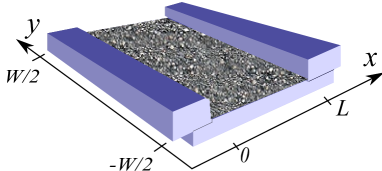
Figure 2: (Color online) The setup for two-terminal transport measurements: a 2D disordered sample of size $W\times L$ with perfect leads attached on opposite sides.

The transport statistics is completely determined by the matrix of transmission amplitudes $t_{mn}$ between channels $m$ and $n$ in the leads since the transmission probabilities of the system are given by the eigenvalues $T_{n}$ of the matrix $\hat{t}^{\dagger}\hat{t}$.beenakker97

The scattering matrix $\mathcal{S}$ relates incoming to outgoing states. An alternative formulation is based on the the transfer matrix $\mathcal{T}$ which relates the states in the left lead to states in the right lead: $c^{\mathrm{right}}=\mathcal{T}c^{\mathrm{left}}$. The waves in the left and the right leads are given by the vectors $c^{\mathrm{left}}=[\{a_{n}^{+}\},\{a_{n}^{-}\}]$ and $c^{\mathrm{right}}=[\{b_{n}^{+}\},\{b_{n}^{-}\}]$, respectively. One can show that the eigenvalues of $\mathcal{TT}^{\dagger}$ appear in pairs of the form $e^{\pm 2\lambda_{n}}$ with $\lambda_{n}\geq 0$ related to the transmission eigenvalues by $T_{n}=1/\cosh^{2}\lambda_{n}$.

The transmission eigenvalues allow one to calculate a variety of transport properties. In the limit of large number of channels one can introduce the distribution function $P(T)$. By definition $\int dTP(T)$ gives the total number of open channels. The first two moments of the distribution give the Landauer conductance

$$G=\frac{e^{2}}{h}\textrm{Tr}\,\hat{t}^{\dagger}\hat{t}=\frac{e^{2}}{h}\int_{0}^{\infty}dT\,TP(T).$$ (32)

and the Fano factor

$$F = 1-\frac{\mathrm{Tr}\,(\hat{t}^{\dagger}\hat{t})^{2}}{\textrm{Tr}\,\hat{t}^{\dagger}\hat{t}}$$ (33)

$$= 1-\left(\int_{0}^{\infty}dTT^{2}P(T)\right)\Big{/}\left(\int_{0}^{\infty}dTTP(T)\right),\ \ \ \$$

which describes the power spectrum of the noise due to discreetness of the charge carriers at zero frequency and average current $I$: $P_{0}=2eFI$. Note, that for graphene one has to multiply Eq. (32) by the factor of 4 accounting for the spin and valley degeneracy. It is also convenient introduce the probability density $\mathcal{P}(\lambda)$ of the parameter $\lambda$ defined by $T=1/\cosh^{2}(\lambda)$, which is naturally completely equivalent to $P(T)$.

In general one can write down an integral equation for the transfer matrix with a kernel which depends on a particular realization of disorder. Iterating the integral equation and averaging over disorder one can compute the transfer matrix as an expansion in small disorder. However, in the case of LR correlated disorder the forthcoming problem of computing the transmission eigenvalues seems to be a formidable task. Fortunately, there is an alternative way which allows one to relate $P(T)$ to the free energy of an auxiliary field theory. This method is based on the matrix Green function formalism introduced by Nazarov.nazarov94 Instead of $P(T)$ the statistics of the transmission eigenvalues can be encoded in the generating function

$$\mathcal{F}(z)=\sum\limits_{n=1}^{\infty}z^{n-1}\mathrm{Tr}(\hat{t}^{\dagger}\hat{t})^{n}=\mathrm{Tr}[\hat{t}^{-1}\hat{t}^{\dagger\,-1}-z]^{-1}.$$ (34)

All moments of $P(T)$ can be computed using the series expansion of $\mathcal{F}(z)$ at $z=0$. The function $\mathcal{F}(z)$ is regular in vicinity of $z=0$ and has a brunch cut along the real axis going from 1 to $\infty$. Both functions are related by the Riemann-Hilbert equation

$$\mathcal{F}(z)=\int_{0}^{1}\frac{P(T)dT}{T^{-1}-z}$$ (35)

and its solution is given by the jump of $\mathcal{F}(z)$ across the brunch cut

$$P(T)=\frac{1}{2\pi iT^{2}}[\mathcal{F}(1/T+i0)-\mathcal{F}(1/T-i0)].$$ (36)

To calculate $\mathcal{F}(z)$ we now adopt the matrix Green functions approach originally developed in Ref. nazarov94, and applied to Dirac fermions in graphene with uncorrelated disorder in Ref. schuessler10, . The coefficients of the series expansion of the generating function at $z=0$ can be expressed in terms of the Green functions of the system as

$$\mathrm{Tr}(\hat{t}^{\dagger}\hat{t})^{n}=\mathrm{Tr}[\hat{v}\hat{G}^{A}(x,x^{\prime})\hat{v}\hat{G}^{R}(x^{\prime},x)]^{n}_{x=0,x^{\prime}=L}.$$ (37)

Here $\hat{v}_{x}=\sigma_{x}\hat{\mathds{1}}$ is the velocity operator and the retarded and advanced Green functions in the channel-coordinate representation read

$$(\epsilon-\hat{H}\pm i0)\hat{G}^{R,A}(x,x^{\prime})=\delta(x-x^{\prime})\hat{\mathds{1}}.$$ (38)

The generating function can be written as a trace of an auxiliary two component Green function defined in the retarded-advanced (RA) space in the presence of fictitious field $z$.nazarov94 The matrix Green function is given by

$$\check{K}(x)\check{G}(x,x^{\prime})=\delta(x-x^{\prime})\check{\mathds{1}},$$ (39)

where we use ”check” notation for the objects defined in RA space and the operator $\check{K}$ reads

$$\check{K}(x)=\left(\begin{array}[]{cc}\epsilon-\hat{H}+i0&-\sqrt{z}\hat{v}\delta(x)\\[8.53581pt] -\sqrt{z}\hat{v}\delta(x-L)&\epsilon-\hat{H}-i0\\ \end{array}\right).$$ (42)

Considering the field $z$ as a small perturbation we can rewrite Eq. (39) in an integral form as follows

$$\check{G}(x,x^{\prime}) = \check{G}_{0}(x,x^{\prime})$$ (43)

$$+\sqrt{z}\int\,dx_{1}\check{G}_{0}(x,x_{1})\check{\mathcal{V}}_{x_{1}}\check{G}(x_{1},x^{\prime})\ \ \ \ \$$

with the kernel and the inhomogeneity given by

$$\check{G}_{0}=\left(\begin{array}[]{cc}\hat{G}^{R}&0\\[8.53581pt] 0&\hat{G}^{A}\\ \end{array}\right),\ \check{\mathcal{V}}_{x}=\left(\begin{array}[]{cc}0&\hat{v}\delta(x)\\[8.53581pt] \hat{v}\delta(L-x)&0\\ \end{array}\right).$$ (48)

One can then compute the generating function using

$$\mathcal{F}(z)=\frac{1}{2\sqrt{z}}\int dx\,\mathrm{Tr}[\check{\mathcal{V}}_{x}\check{G}(x,x)]$$ (49)

that can be checked by iterating Eq. (43) and substituting in Eq. (49). One can relate $\mathcal{F}(z)$ to the object which plays the role of the free energy in the corresponding field theory. Let us rewrite the Green function (39) in coordinate representation using a functional integral over Grassmann variables $\bar{\psi}$ and $\psi$

$$\check{G}(\mathbf{r},\mathbf{r}^{\prime})=\frac{1}{Z}\int\mathcal{D}\bar{\psi}\mathcal{D}\psi\,\bar{\psi}(\mathbf{r})\psi(\mathbf{r}^{\prime})\,e^{-S}$$ (50)

with the bilinear in $\bar{\psi}$ and $\psi$ action

$$S=\int d^{2}\mathbf{r}[\bar{\psi}(\mathbf{r})\check{K}\psi(\mathbf{r})].$$ (51)

The corresponding partition function and the free energy can be written as follows

$$Z(z)=\mathrm{Det}\,K=\int\mathcal{D}\bar{\psi}\mathcal{D}\psi\,e^{-S},\ \ \ \Omega(z)=\ln Z.$$ (52)

It is convenient to rewrite the free energy in terms of the angle $\phi$ defined by $z=\sin^{2}(\phi/2)$. Direct inspection of Eq. (43) shows that

$$\mathcal{F}(z)=\frac{\partial\Omega(z)}{\partial z}=\left.\frac{2}{\sin\phi}\frac{\partial\Omega(\phi)}{\partial\phi}\right|_{\phi=2\arcsin\sqrt{z}}.$$ (53)

The distribution of transmission eigenvalues $\mathcal{P}(\lambda)$ can be calculated using the following relation

$$\mathcal{P}(\lambda)=\left.\frac{2}{\pi}\mathrm{Re}\frac{\partial\Omega(\phi)}{\partial\phi}\right|_{\phi=\pi+2i\lambda},$$ (54)

from which one can easily derive $P(T)$. Therefore, we have four equivalent descriptions of the transport properties in terms of one of the following functions: $P(T)$, $\mathcal{P}(\lambda)$, $\mathcal{F}(z)$ or $\Omega(\phi)$. Any of these functions can be used for computing the conductance or the Fano factor. For instance, using the free energy one can derive the expressions

$$G=\frac{2e^{2}}{h}\Omega^{\prime\prime}(0),\ \ \ F=\frac{1}{3}-\frac{2}{3}\frac{\Omega^{(\mathrm{{IV}})}(0)}{\Omega^{\prime\prime}(0)},$$ (55)

where the derivatives are taken at $\phi=0$. Note that in the case of graphene the conductance (55) is given as expected per Dirac species, i.e. per spin and per valley.

IV.2 Expansion in disorder and diagrammatics

In what follows we restrict our consideration to transport around the Dirac cone $\epsilon=0$. The action (51) for the system including the metallic leads can be calculated using the kernel (42) with Hamiltonian (1) in which the free part is modified to

$$H_{0}=-\mu(x)-iv_{0}(\sigma_{x}\partial_{x}+\sigma_{y}\partial_{y}).$$ (56)

Here $\mu(x)=0$ for $0<x<L$ and $+\infty$ otherwise accounts for the leads with very high chemical potential. Above we have treated the auxiliary field $z$ as a perturbation. Here we split the kernel (42) into the free part including the auxiliary field and the interaction part: $\check{K}=\check{K}_{0}+\check{K}_{V}$, where $\check{K}_{0}$ is computed using Eq. (56) and $\check{K}_{V}$ is diagonal in RA space.

Figure 3: The one-loop diagrams contributing to (a) free energy; (b) propagator; (c)-(e) disorder renormalization.

We are now in the position to average the free energy over disorder. To that end we use the replica trick and introduce $n$ copies of the original system. Performing averaging over disorder we obtain the replicated action in the following form

$$S = \sum\limits_{\alpha=1}^{n}\int d^{2}\mathbf{r}\bar{\psi}_{\alpha}(\mathbf{r})\check{K}_{0}\psi_{\alpha}(\mathbf{r})$$ (57)

$$+\pi v_{0}^{2}\sum\limits_{\alpha,\beta=1}^{n}\sum\limits_{\mu=0}^{3}\int d^{2}\mathbf{r}\int d^{2}\mathbf{r}^{\prime}g_{\mu}(\mathbf{r}-\mathbf{r}^{\prime})$$

$$\times[\bar{\psi}_{\alpha}(\mathbf{r})\Sigma_{\mu}\psi_{\alpha}(\mathbf{r})][\bar{\psi}_{\beta}(\mathbf{r})\Sigma_{\mu}\psi_{\beta}(\mathbf{r})]$$

where $\check{K}_{0}$ is given by Eq. (42) with Hamiltonian (56) and we defined the matrix $\Sigma_{\mu}=\check{\mathds{1}}\otimes\sigma_{\mu}$. In what follows we set $v_{0}=1$ unless it is written explicitly. The bare Green function corresponding to $\check{K}_{0}$ in Eq. (39) can be written in coordinate representation as

$$G_{0}(x,x^{\prime};y)=\frac{1}{4L\cos(\phi/2)}\times$$

$$\left(\begin{array}[]{cccc}\frac{\cos\phi(\frac{1}{2}-x^{0}_{0})}{i\sin\pi x^{0}_{0}}&\frac{\cos\phi(\frac{1}{2}-x^{1}_{0})}{i\sin\pi x^{1}_{0}}&\frac{\sin\phi(1-x^{0}_{0})}{\sin\pi x^{0}_{0}}&\frac{\sin\phi x^{1}_{0}}{\sin\pi x^{1}_{0}}\\ \frac{\cos\phi(\frac{1}{2}-x^{1}_{1})}{i\sin\pi x^{1}_{1}}&\frac{\cos\phi(\frac{1}{2}-x^{0}_{1})}{i\sin\pi x^{0}_{1}}&\frac{\sin\phi x^{1}_{1}}{\sin\pi x^{1}_{1}}&\frac{\sin\phi(1-x^{0}_{1})}{\sin\pi x^{0}_{1}}\\ \frac{\sin\phi x^{0}_{0}}{\sin\pi x^{0}_{0}}&\frac{\sin\phi x^{1}_{0}}{\sin\pi x^{1}_{0}}&\frac{i\cos\phi(\frac{1}{2}-x^{0}_{0})}{\sin\pi x^{0}_{0}}&\frac{\cos\phi(\frac{1}{2}+x^{1}_{0})}{i\sin\pi x^{1}_{0}}\\ \frac{\sin\phi x^{1}_{1}}{\sin\pi x^{1}_{1}}&\frac{\sin\phi x^{0}_{1}}{\sin\pi x^{0}_{1}}&\frac{\cos\phi(\frac{1}{2}+x^{1}_{1})}{i\sin\pi x^{1}_{1}}&\frac{i\cos\phi(\frac{1}{2}-x^{0}_{1})}{\sin\pi x^{0}_{1}}\end{array}\right),$$ (62)

(63)

where we have introduced the shorthand notation $x^{k}_{l}=(x+(-1)^{k}x^{\prime}+(-1)^{l}iy)/2L$.

We will first reproduce the known results for the free Dirac fermions i.e. for clean graphene. To that end we rewrite the free energy (49) in the coordinate representation as a function of $\phi$:

$$\mathcal{F}(\phi)=\frac{W}{2\sin\phi/2}\int dx\,\mathrm{Tr}\left[\check{\mathcal{V}}_{x}\check{G}_{0}(x,x,0)\right].$$ (64)

Substituting the bare Green function (63) we obtain the generating function and the corresponding free energy

$$\mathcal{F}_{0}(z)=\frac{W\arcsin\sqrt{z}}{\pi L\sqrt{z-z^{2}}},\ \ \ \ \Omega_{0}(\phi)=\frac{W\phi^{2}}{4\pi L}.$$ (65)

The corresponding distribution of transmission eigenvalues then reads

$$P_{0}(T)=\frac{W}{2\pi L}\frac{1}{T\sqrt{1-T}}.$$ (66)

The distribution $P(T)$ is expected to be integrable and the integral gives the total number of open channels. However the integral of Eq. (66) diverges logarithmical at $T=0$: we need to introduce a cutoff $T_{\mathrm{min}}\sim e^{-2\epsilon L/v_{0}}$. However, the contribution of this cutoff to the higher moments is found to be exponentially small. Equation (66) coincides with the well-known result obtained by Dorokhov for the disordered metallic wires.dorokhov83 Thus, the transport of clean 2D Dirac fermions resembles the diffusive transport of non-relativistic electrons in quasi-one-dimensional systems in the presence of disorder. This nontrivial result can be explained by existence of the evanescent modes.

IV.3 The lowest order correction to free energy

The perturbative corrections to the free energy of the system due to disorder can be expressed as a sum of loop diagrams without external legs. The lowest order contributions to the free energy are given by the one loop diagrams schematically shown in Fig. 3(a). The solid lines denote the propagator (63) in the presence of the boundary auxiliary field $\phi$ and the dashed lines stands for disorder correlation functions. There are six topologically equivalent diagrams with different disorder correlators corresponding to SR and LR correlated disorder of three types: random potential, random gauge (with two components $x$ and $y$) and random mass. The corresponding integrals have the form

$$\Omega_{\mathrm{SR,LR}}=\pi\int d^{2}\mathbf{r}d^{2}\mathbf{r}^{\prime}g_{\mu}(\mathbf{r}-\mathbf{r}^{\prime})\mathrm{Tr}[\check{\Sigma}_{\mu}\check{G}(\mathbf{r},\mathbf{r}^{\prime})\check{\Sigma}_{\mu}\check{G}(\mathbf{r}^{\prime},\mathbf{r})].$$ (67)

with $g_{\mu}(\mathbf{r})$, $\mu=0,x,y,z$ given by Eq. (6) where we retain only the SR or LR part. These integrals diverge for $\mathbf{r}\to\mathbf{r}^{\prime}$, however, the divergent terms turn out to be $\phi$-independent, and thus do not contribute to the physical quantities (55). Hence, it is convenient to consider the first derivative of the free energy with respect to $\phi$ which is finite and determines the physical observables. The $\phi$-dependent parts of diagrams with dashed line corresponding to the three types of SR correlated disorder were computed in Ref. schuessler10, . The result giving the linear in $\alpha_{\mu}$ correction to the free energy of the clean sample (65) reads

$$\Omega^{\prime}_{\mathrm{SR}}(\phi)=\frac{W\phi}{2\pi L}\left(\alpha_{0}-\alpha_{z}\right).$$ (68)

Note that the SR correlated random gauge potential does not contribute to the transport properties to one-loop order and this holds also to two-loop order. This is in agreement with the arguments of Ref. schuessler10, that at zero energy the gauge potential can be eliminated by a pseudogauge transformation of the wave function. As a result, the transport properties are not influenced by random gauge potential despite the fact that it gives rise to a multifractal wave function $\Psi(\mathbf{r})$ with a disorder strength dependent spectrum of multifractal exponents.ludwig94 ; chamon96 ; castillo97 ; comtet98 ; carpentier01

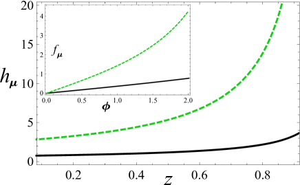
Figure 4: (Color online) The one-loop LR disorder corrections to the generating function of transmissions (75) for $a=1$: $h_{0}(z)$ - solid black line and $h_{z}(z)$ - dashed green line. Inset. The one-loop LR disorder corrections to the free energy (LABEL:eq:free-energy-02) for $a=1$: $f_{0}(\phi)$ - solid black line and $f_{z}(\phi)$ - dashed green line.

The three diagrams with dashed line associated with correlation functions of the LR correlated disorder are computed in Appendix A. The corresponding corrections to the free energy read

$$\Omega^{\prime}_{\mathrm{LR}}(\phi) = \frac{W}{2\pi L^{a-1}}\left[f_{0}(\phi)\beta_{0}-f_{z}(\phi)\beta_{z}\right].$$

We found that the LR correlated random gauge potential does not contribute to the transport properties to lowest order in disorder strength. The functions $f_{\mu}(\phi)$ are given by the following double integrals:

$$f_{0,z}(\phi)=\int\limits_{0}^{\infty}dy\int\limits_{0}^{\pi}dc\frac{4\pi^{a-2}\mathcal{A}_{a}y\sinh(y\phi/\pi)}{\left(c^{2}+y^{2}\right)^{a/2}}$$

$$\times\left\{\pm\frac{1}{\sinh y}\right.\left[\arctan\left(\frac{1-\cos c\cosh y}{\sin c\sinh y}\right)-\frac{\pi}{2}\right]$$

$$\left.+\frac{\pi-c}{\cosh y-\cos c}\right\},$$ (70)

where the upper sign corresponds to $f_{0}(\phi)$ and the lower sign to $f_{z}(\phi)$. The functions $f_{\mu}(\phi)$ computed numerically for a particular value of $a=1$ are shown in inset of Fig. 4.

Figure 5: (Color online) The one-loop LR disorder corrections to the conductance (77) as functions of $a$: $f_{0}^{\prime}(0)$ - solid black line and $f_{z}^{\prime}(0)$ - dashed green line.

It is known that even in the case of uncorrelated disorder the lowest order corrections to the density of states and the transport properties of 2D Dirac fermions are insufficient. The leading corrections can be summed up with the help of the renormalization group methods that will be done in the next section.

V Weak disorder renormalization group

Straightforward dimensional analysis shows that the SR correlated disorder is dimensionless and hence marginally relevant in $d=2$. The LR correlated disorder is relevant in $d=2$ for $a<2$. In what follows it is convenient to introduce the rescaled disorder strengths: $\alpha(L)=\tilde{\alpha}(L)$ and $\beta(L)=\tilde{\beta}(L)L^{a-2}$. The lowest order corrections to the disorder strength and energy are given by the one-loop diagrams (b)-(e) shown in Fig. 3. The corresponding RG flow equations read

$$\frac{\partial\tilde{\alpha}_{0}}{\partial\ln L} = 2\tilde{\alpha}_{0}(\tilde{\alpha}_{0}+\tilde{\beta}_{0}+\tilde{\alpha}_{\bot}+\tilde{\beta}_{\bot}+\tilde{\alpha}_{z}+\tilde{\beta}_{z})$$ (71a)

$$+2(\tilde{\alpha}_{\bot}+\tilde{\beta}_{\bot})(\tilde{\alpha}_{z}+\tilde{\beta}_{z}),$$

$$\frac{\partial\tilde{\beta}_{0}}{\partial\ln L} = (2-a)\tilde{\beta}_{0}+2\tilde{\beta}_{0}(\tilde{\alpha}_{0}+\tilde{\beta}_{0}+\tilde{\alpha}_{\bot}+\tilde{\beta}_{\bot}$$ (71b)

$$+\tilde{\alpha}_{z}+\tilde{\beta}_{z}),$$

$$\frac{\partial\tilde{\alpha}_{\bot}}{\partial\ln L} = 4(\tilde{\alpha}_{0}+\tilde{\beta}_{0})(\tilde{\alpha}_{z}+\tilde{\beta}_{z}),$$ (71c)

$$\frac{\partial\tilde{\beta}_{\bot}}{\partial\ln L} = (2-a)\tilde{\beta}_{\bot},$$ (71d)

$$\frac{\partial\tilde{\alpha}_{z}}{\partial\ln L} = -2\tilde{\alpha}_{z}^{2}-2\tilde{\alpha}_{z}\tilde{\beta}_{z}+2(\tilde{\alpha}_{z}+\tilde{\alpha}_{0}+\tilde{\beta}_{0})(\tilde{\alpha}_{\bot}+\tilde{\beta}_{\bot})$$ (71e)

$$-2\tilde{\alpha}_{z}(\tilde{\alpha}_{0}+\tilde{\beta}_{0}),$$

$$\frac{\partial\tilde{\beta}_{z}}{\partial\ln L} = (2-a)\tilde{\beta}_{z}-2\tilde{\beta}_{z}^{2}-2\tilde{\alpha}_{z}\tilde{\beta}_{z}$$ (71f)

$$+2\tilde{\beta}_{z}(\tilde{\alpha}_{\bot}+\tilde{\beta}_{\bot}-\tilde{\alpha}_{0}-\tilde{\beta}_{0}),$$

$$\frac{\partial\ln\tilde{\varepsilon}}{\partial\ln L} = 1+\tilde{\alpha}_{0}+\tilde{\beta}_{0}+\tilde{\alpha}_{\bot}+\tilde{\beta}_{\bot}+\tilde{\alpha}_{z}+\tilde{\beta}_{z},$$ (71g)

where we used the notation $\tilde{\alpha}_{\bot}=\tilde{\alpha}_{x}+\tilde{\alpha}_{y}$ and $\tilde{\beta}_{\bot}=\tilde{\beta}_{x}+\tilde{\beta}_{y}$. Note, that in deriving the flow equations (71) we assume that $2-a$ is small and perform $2-a$ expansion similar to $d-2$ expansion in higher dimensions. In general in the presence of LR correlated disorder one has to rely on the double expansion in $2-a$ and $d-2$ similar to that for the $\phi^{4}$ model with correlated random bond disorder where one uses a double expansion in $4-a$ and $4-d$ at the upper critical dimension.weinrib83

The bare values of the disorder strengths and energy corresponding to the microscopic scale provide the initial condition for the RG equations (71). The renormalized disorder strengths, $\alpha(L)$, $\beta(L)$, and the energy $\varepsilon(L)$ acquire scale dependence on the ultraviolet cutoff length $L$. One has to stop the renormalization when either $L$ reaches the system size or the energy $\tilde{\varepsilon}$ reaches the value of the cutoff $\Delta$ or the disorder strengths become of order one.schuessler09 Once the renormalization has been done one can compute the observables by substituting the renormalized quantities into the results of the perturbation theory.

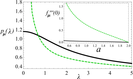
Figure 6: (Color online) The LR correlated disorder corrections to the transmission eigenvalue distribution $P(\lambda)$ given by Eq. (76) for $a=1.5$: $p_{0}(\lambda)$ - solid black line and $p_{z}(\lambda)$ - dashed green line as a function of $\lambda$. Inset. The LR correlated disorder corrections to the Fano factor given by Eq. (78): $f_{0}^{\prime\prime\prime}(0)$ - solid black line and $f_{z}^{\prime\prime\prime}(0)$ - dashed green line, as functions of $a$.

To renormalize the corrections to the free energy (68) and (LABEL:eq:free-energy-02) we have to replace the bare coupling constants by the renormalized ones. As a result we obtain

$$\Omega^{\prime}_{\mathrm{SR}}(\phi) = \frac{W\phi}{2\pi L}\left[\tilde{\alpha}_{0}(L)-\tilde{\alpha}_{z}(L)\right],$$ (72)

$$\tilde{\Omega}^{\prime}_{\mathrm{LR}}(\phi) = \frac{W}{2\pi L}\left[f_{0}(\phi)\tilde{\beta}_{0}(L)-f_{z}(\phi)\tilde{\beta}_{z}(L)\right].\$$ (73)

Thus, the SR correlated disorder does not modify the pseudodiffusive behavior to lowest order ($\Omega\sim\phi^{2}$) and the distributions of transmission eigenvalues is still given by the Dorokhov distribution (66). The deviation from the pseudodiffusive regime can be found only to second order in disorder and the corresponding two-loop corrections have the formschuessler10

$$\Omega_{\mathrm{SR}}^{\mathrm{2loop}} = \frac{W\phi^{2}}{4\pi L}[(\tilde{\alpha}_{0}+\tilde{\alpha}_{z})^{2}\omega_{1}(\phi)$$ (74)

$$+(\tilde{\alpha}_{0}+3\tilde{\alpha}_{z})(\tilde{\alpha}_{0}-\tilde{\alpha}_{z})]\omega_{2}(\phi),$$

where $\omega_{1}(\phi)=\mathrm{const}-\psi(\phi/\pi)-\psi(-\phi/\pi)$ and $\omega_{2}(\phi)=\mathrm{const}+\pi^{2}(\phi\cot\phi-1)/\phi^{2}$. Here $\psi(x)$ is the digamma function.olver2010

On the contrary the LR correlated disorder leads to deviation from pseudodiffusive transport already to lowest order in disorder. Indeed the renormalized corrections to the generating function and the distribution of transmission eigenvalues read

$${\mathcal{F}}_{\mathrm{LR}}(z) = \frac{W}{2\pi L}\left[h_{0}(z)\tilde{\beta}_{0}-h_{z}(z)\tilde{\beta}_{z}\right],\$$ (75)

$${\mathcal{P}}_{\mathrm{LR}}(\lambda) = \frac{W}{2\pi L}\left[p_{0}(\lambda)\tilde{\beta}_{0}-p_{z}(\lambda)\tilde{\beta}_{z}\right].\$$ (76)

Here $h_{\mu}(z)=2f_{\mu}(2\arcsin\sqrt{z})/\sin\phi$ and $p_{\mu}(\lambda)=2\mathrm{Re}f_{\mu}(\pi+2i\lambda)/\pi$. The functions $h_{\mu}(z)$ and $p_{\mu}(\lambda)$ for particular values of $a$ are shown in Figs. (4) and (6). Note that the distribution (76) can be used for direct calculation of transmissions moments for $1<a<2$. This is different from the two-loop correction (74) due to SR correlated disorder found in Ref. schuessler10, : the corresponding contributions to $\mathcal{P}(\lambda)$ diverge at $\lambda=0$ in a non-integrable way. This divergence has been attributed to the breakdown of perturbative expansion in small disorder close to $\lambda=0$, i.e. for $T\approx 1$. Nevertheless even for $a\leq 1$ one can compute the transport characteristics directly from the free energy. The correction to the conductance is given by

$$G_{\mathrm{LR}}=\frac{e^{2}W}{\pi hL}\left[f^{\prime}_{0}(0)\tilde{\beta}_{0}-f^{\prime}_{z}(0)\tilde{\beta}_{z}\right].$$ (77)

and the Fano factor can be written as

$$F=\frac{1}{3}-\left.\frac{2}{3}\frac{f^{\prime\prime\prime}_{0}\tilde{\beta}_{0}-f^{\prime\prime\prime}_{z}\tilde{\beta}_{z}}{1+\alpha_{0}-\alpha_{z}+f^{\prime}_{0}\tilde{\beta}_{0}-f^{\prime}_{z}\tilde{\beta}_{z}}\right|_{\phi=0}.\ \ \ \ \ \$$ (78)

$f_{\mu}^{\prime}(0)$ and $f_{\mu}^{\prime\prime\prime}(0)$ as functions of $a$ are shown in Figs. (5) and (6), respectively. The case of generic disorder requires a numerical solution of the flow equations which strongly depends on the particular values of bare couplings. In the present paper we restrict our analysis to three cases when the system has only one type of disorder: random scalar potential, random gauge potential or random mass disorder.

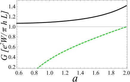
Figure 7: (Color online) The conductance as a function of $a$ in the presence of random potential for $L/l_{0}=0.5$ - solid black line and in the presence of random mass - dashed green line.

V.1 Random scalar disorder

Let us start the discussion of the different types of disorder with random scalar potential. In the presence of both SR and LR correlated scalar potential the solution of the flow equations

$$\frac{\partial\tilde{\alpha}_{0}}{\partial\ln L} = 2\tilde{\alpha}_{0}(\tilde{\alpha}_{0}+\tilde{\beta}_{0}),$$ (79)

$$\frac{\partial\tilde{\beta}_{0}}{\partial\ln L} = (2-a)\tilde{\beta}_{0}+2\tilde{\beta}_{0}(\tilde{\alpha}_{0}+\tilde{\beta}_{0}),$$ (80)

$$\frac{\partial\ln\tilde{\varepsilon}}{\partial\ln L} = 1+\tilde{\alpha}_{0}+\tilde{\beta}_{0},$$ (81)

can be computed only numerically. However, we have found that the LR correlated disorder dominates over SR correlated disorder at large $L$ for all bare disorder strengths such that $\tilde{\alpha}\leq\tilde{\beta}$. Since LR correlated disorder does not generate SR disorder itself we restrict ourselves to the case of pure LR disorder. Here and below we will measure the length in units of the bare ultraviolet cutoff given by $v_{0}/\Delta$. The solution of the flow equation (80) with the initial conditions $\tilde{\beta}_{0}(1)=\bar{\beta}_{0}=\beta(\Delta/v_{0})^{a-2}$ reads

$$\tilde{\beta}_{0}(L)=(a-2)\left[2+L^{a-2}(a-2(1+\bar{\beta}_{0}))/\bar{\beta}_{0})\right]^{-1}.$$ (82)

The running disorder strength grows with the scale. At the Dirac cone the renormalization has to be stopped either at the scale of the system size or at the scale at which the disorder strength becomes of order unity. This scale computed from Eq. (82) reads

$$l_{0}=\left(\frac{2-a+2\bar{\beta}_{0}}{(4-a)\bar{\beta}_{0}}\right)^{1/(2-a)}.$$ (83)

$l_{0}$ is nothing but the zero-energy mean free path. For the system size $L<l_{0}$ one can rewrite the running disorder strength in terms of $l_{0}$ as follows

$$\tilde{\beta}_{0}(L)=\frac{(2-a)}{(4-a)(l_{0}/L)^{2-a}-2}.$$ (84)

For finite energy the renormalization is limited by the scale at which the energy becomes of order of $\Delta$. Substitution of the solution (82) to the flow equation for the energy (81) yields

$$\tilde{\varepsilon}(L)=\varepsilon L\left[1-2\bar{\beta}_{0}(L^{a-2}-1)/(a-2)\right]^{-1/2}.$$ (85)

The renormalization stops when the running energy $\tilde{\varepsilon}(L)$ reaches the cutoff value $\Delta$ at the scale

$$L_{\Delta}(\varepsilon)=\frac{\Delta}{\varepsilon}\left[1-2\bar{\beta}_{0}((\Delta/|\varepsilon|)^{a-2}-1)/(a-2)\right]^{1/2}.$$ (86)

The competition between $L_{\Delta}$ and $l_{0}$ introduces a new exponentially small (in the limit $a\to 2$) in disorder energy scale $\Gamma_{2-a}$ given by equation $L_{\Delta}(\Gamma_{2-a})=l_{0}$,

$$\!\!\!\!\!\Gamma_{2-a}=\Delta\,l_{0}^{-1}\,\sqrt{\frac{a-2-2\bar{\beta}_{0}^{2}}{a-2-2\bar{\beta}_{0}}}\approx\Delta e^{-\frac{1}{2\bar{\beta}_{0}}+\frac{1}{2}}{\bar{\beta}_{0}}^{1/2}$$

$$\!\!\!\!\!\times\left[1+(2-a)\left(\frac{3}{8\bar{\beta}_{0}^{2}}-\frac{1}{4\bar{\beta}_{0}}-\frac{1}{8}\right)+O((2-a)^{2})\right].\ \ \ \$$ (87)

For $\varepsilon\gg\Gamma_{2-a}$ the density of states can be found using the following scaling arguments. The running density of states approaches $\tilde{\rho}=\Delta/(2\pi v_{0}^{2})$ at $L=L_{\Delta}$. Taking into account that the density of states scales as $\tilde{\rho}\tilde{\varepsilon}=\rho\varepsilon L^{2}$ one can write the bare density of states as

$$\rho(\varepsilon)=\frac{|\varepsilon|}{2\pi v_{0}^{2}}\left[1-2\bar{\beta}_{0}((\Delta/|\varepsilon|)^{a-2}-1)/(a-2)\right]^{-1}.$$ (88)

For $\varepsilon<\Gamma_{2-a}$ the density of states saturates at a finite value. This picture is in qualitative agreement with the prediction of SCBA computed in Sec. III. The results for SR correlated disorder case obtained in Ref. ostrovsky06, can be reproduced by taking the limit of $a\to 2$. For instance, in this limit we have $\Gamma_{0}\approx\Delta\,{\bar{\beta}_{0}}^{1/2}e^{-1/2\bar{\beta}_{0}}$.

The conductance and the Fano factor in the ballistic regime $L<l_{0}$ at the Dirac cone are given by

$$G = \frac{e^{2}}{\pi h}\frac{W}{L}\left[1+f_{0}^{\prime}(0)\ \tilde{\beta}_{0}\left(L\right)\right],$$ (89)

$$F = \frac{1}{3}-\frac{2}{3}\frac{f^{\prime\prime\prime}_{0}(0)\tilde{\beta}_{0}(L)}{1+f^{\prime}_{0}(0)\tilde{\beta}_{0}(L)},$$ (90)

where $\tilde{\beta}_{0}(L)$ is given by Eq. (84). The conductance and the Fano factor computed for $L/l_{0}=0.5$ are shown in Figs. (7) and (8) as functions of $a$. The correction to the conductance due to LR correlated disorder in the ballistic regime is positive and increases with $a$ while the correction to the Fano factor is small and negative.

V.2 Random gauge potential

We now turn to the case of random gauge potential. Inspired mostly by its relation to the Quantum Hall transitions,ludwig94 this problem has previously motivated numerous studies of the multifractal spectrum for critical wave functions.chamon96 ; castillo97 ; comtet98 ; carpentier01 Here we are mostly interested in the density of states and also transport properties of such Dirac fermions with correlated random gauge potential. In this case the flow equations reduce to

$$\frac{\partial\tilde{\alpha}_{\bot}}{\partial\ln L} = 0,\ \ \ \frac{\partial\tilde{\beta}_{\bot}}{\partial\ln L}=(2-a)\tilde{\beta}_{\bot},$$ (91)

$$\frac{\partial\ln\tilde{\varepsilon}}{\partial\ln L} = 1+\tilde{\alpha}_{\bot}+\tilde{\beta}_{\bot}.$$ (92)

The renormalized coupling constants have the trivial flow $\tilde{\alpha}_{\bot}(L)=\bar{\alpha}_{\bot}$ and $\tilde{\beta}_{\bot}(L)=\bar{\beta}_{\bot}L^{2-a}$ where the bare disorder strengths are $\bar{\alpha}=\alpha$ and $\bar{\beta}_{\bot}={\beta}_{\bot}(\Delta/v_{0})^{a-2}$. The LR disorder strength reaches unity at the scale $l_{0}=\bar{\beta}_{\bot}^{-1/(2-a)}$. Substituting the running couplings to the flow equation for the energy (92) we obtain

$$\tilde{\varepsilon}(L)=\varepsilon L^{1+\bar{\alpha}_{\bot}}\exp\left[\tilde{\beta}_{\bot}(L^{2-a}-1)/(2-a)\right].$$ (93)

One has to stop renormalization at the scale $L_{\Delta}$ such that $\tilde{\varepsilon}(L_{\Delta})=\Delta$. In the case of the system with only SR correlated random gauge disorder this scale is given by $L_{\Delta}^{\mathrm{SR}}=\left({\varepsilon}/{\Delta}\right)^{-1/z}$, where we have introduced the dynamic critical exponent $z=1+\bar{\alpha}_{\bot}$. Note that this exponent is non-universal and depends on the strength of disorder. In the presence of LR correlated disorder the cutoff scale computed up to subleading logarithmic corrections is

$$L_{\Delta}^{\mathrm{LR}}=\left(\frac{2-a}{\bar{\beta}_{\bot}}\ln\frac{\Delta}{\varepsilon}\right)^{1/(2-a)}.$$ (94)

However, one has to stop renormalization at $l_{0}$ for $l_{0}<L_{\Delta}^{\mathrm{LR}}$ that introduces a new energy scale $\Gamma_{2-a}=\Delta e^{-1/(2-a)}$ which is exponentially small for $a\to 2$. The bare density of states is then given by $\rho=\tilde{\rho}\tilde{\varepsilon}/(\varepsilon L_{\Delta}^{2})$ with $\tilde{\rho}=\Delta/(2\pi v_{0}^{2})$. Substituting the renormalized cutoff scale we obtain for the SR correlated disorder a non-universal power-law behavior:

$$\rho_{\mathrm{SR}}(\varepsilon) = \frac{\Delta}{2\pi v_{0}^{2}}\left(\frac{\varepsilon}{\Delta}\right)^{(2-z)/z},\ \ \ z=1+\bar{\alpha}_{\bot}$$ (95)

which was firstly derived in Ref. ludwig94, . In the case of LR random gauge disorder we have

$$\rho_{\mathrm{LR}}(\varepsilon) = \frac{\Delta^{2}}{2\pi v_{0}^{2}}\frac{1}{\varepsilon}\left(\frac{2-a}{\bar{\beta}_{\bot}}\ln\frac{\Delta}{\varepsilon}\right)^{-2/(2-a)}$$ (96)

$$= \frac{1}{2\pi\varepsilon}\left(\frac{2-a}{{\beta}_{\bot}}\ln\frac{\Delta}{\varepsilon}\right)^{-2/(2-a)},$$

where in the last line we used the definition of the dimensionless disorder strength so that the dependence on the ultraviolet cutoff drops out from the density of states. Presumably Eq. (96) is valid only for $\varepsilon>\Gamma_{2-a}$. In Sec. VI we apply bosonisation technique to compute the density of states down to zero energy and show that the scaling behavior (96) actually holds up down to zero energy.

We have found above that the LR correlated random gauge disorder does not contribute to transport at the Dirac cone. There are some general arguments that any random gauge potential cannot modify the transport properties. Let us first briefly recall the argument of Ref. schuessler09, . To start, we consider the Hamiltonian (1)-(2) with only a gauge field $\vec{A}$:

$$-iv_{0}\vec{\sigma}\cdot\left(\vec{\nabla}+e\vec{A}\right)\Psi=E\Psi.$$ (97)

It is known from vector analysis that any vector can be decomposed into the sum of a gradient and a rotational. Using that property, we can express the 2D vector $\vec{A}$ as

$$\vec{A}=\vec{\nabla}\chi+(\hat{z}\times\vec{\nabla})\phi.$$ (98)

Using this decomposition, we can rewrite $\vec{\sigma}\cdot\vec{A}$ in the form

$$\vec{\sigma}\cdot\vec{A}=\vec{\sigma}\cdot\vec{\nabla}\chi+\vec{\sigma}\cdot(\hat{z}\times\vec{\nabla})\phi.$$ (99)

The mixed product $\vec{\sigma}\cdot(\hat{z}\times\vec{\nabla}\phi)=(\vec{\sigma}\times\hat{z})\cdot\vec{\nabla}\phi$, and $i\vec{\sigma}\sigma_{z}=(\vec{\sigma}\times\hat{z})$ so the Dirac equation (97) can be rewritten as:

$$-v_{0}\vec{\sigma}\cdot\left(\vec{\nabla}+e\vec{\nabla}\chi+ie\sigma_{z}\vec{\nabla}\phi\right)\Psi=E\Psi.$$ (100)

Then, a pseudogauge transformation to a new wave function $\tilde{\Psi}$ according to

$$\Psi=e^{e(i\chi-\sigma_{z}\phi)}\tilde{\Psi},$$ (101)

turns the Dirac equation (100) into the free Dirac equation without vector potential

$$-iv\vec{\sigma}\cdot\vec{\nabla}\tilde{\Psi}=E\tilde{\Psi},$$ (102)

and thus the transport properties of the initial model (97) turn out to be the same as in the absence of the gauge potential.

However, there are some subtleties in applying this argument to correlated in space gauge potential. The difficulty stems from the fact that the transformation (101) is not unitary. Indeed, if we denote the original and the transformed wave functions by

$$\Psi(x,y)=\left(\begin{array}[]{c}u(x,y)\\ v(x,y)\end{array}\right),\ \ \ \tilde{\Psi}(x,y)=\left(\begin{array}[]{c}\tilde{u}(x,y)\\ \tilde{v}(x,y)\end{array}\right).$$ (103)

Then, the normalization condition

$$1=\int dxdy[|u(x,y)|^{2}+|v(x,y)|^{2}],$$ (104)

transforms under pseudogauge transformation to

$$1=\int dxdy[e^{-2e\phi(x,y)}|\tilde{u}(x,y)|^{2}+e^{2e\phi(x,y)}|\tilde{v}(x,y)|^{2}].$$ (105)

Therefore, the normalization condition (105) is equivalent to the normalization condition (104) only for extended states, and only when $\phi(x,y)$ is vanishing outside of a finite area. Indeed, in that case the normalization integral is dominated by the asymptotic behavior of the extended wavefunctions outside the finite area and is thus unchanged by the transformation.

Thus, if $\phi(x,y)$ is vanishing outside of a finite region, this would also imply a vanishing gradient and thus vanishing correlations of the vector potential outside of this region. As a result, the correlations of the vector potential become necessarily finite ranged, in contradiction with the hypothesis of an infinite ranged power-law decay. This is in contrast with the case of a $\delta$-correlated gauge potential which is compatible with a potential existing only in a finite region of space. Nevertheless, we have not found any corrections to transport to one-loop order.

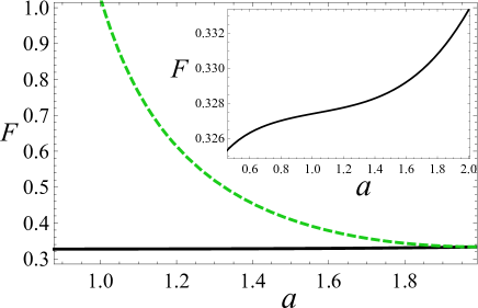
Figure 8: (Color online) The Fano factor as a function of $a$ in the presence of random potential for $L/l_{0}=0.5$ - solid black line (also Inset) and random mass - dashed green line.

V.3 Random mass disorder

Let us now consider the system with only random mass disorder. The corresponding flow equations are

$$\frac{\partial\tilde{\alpha}_{z}}{\partial\ln L} = -2\tilde{\alpha}_{z}^{2}-2\tilde{\alpha}_{z}\tilde{\beta}_{z},$$ (106)

$$\frac{\partial\tilde{\beta}_{z}}{\partial\ln L} = (2-a)\tilde{\beta}_{z}-2\tilde{\beta}_{z}^{2}-2\tilde{\alpha}_{z}\tilde{\beta}_{z},$$ (107)

$$\frac{\partial\ln\tilde{\varepsilon}}{\partial\ln L} = 1+\tilde{\alpha}_{z}+\tilde{\beta}_{z}.$$ (108)

In the case of SR correlated disorder the running disorder strength approaches the Gaussian fixed point ($\tilde{\alpha}_{z}^{*}=0$) so that the SR disorder is marginally irrelevant. This results in the logarithmic corrections to the scaling of the density of states

$$\rho_{\mathrm{SR}}(\varepsilon) = \frac{\alpha_{z}\,\varepsilon}{\pi v_{0}^{2}}\ln\frac{\Delta}{\varepsilon}.$$ (109)

In the most general case the flow equations possess beside the unstable Gaussian fixed point ($\tilde{\alpha}_{z}^{*}=\tilde{\beta}_{z}^{*}=0$) a nontrivial infrared stable fixed point ($\tilde{\alpha}_{z}^{*}=0$, $\tilde{\beta}_{z}^{*}=(2-a)/2$) with eigenvalues $\lambda_{1,2}=-2+a$ negative for $a<2$. The dynamic exponent describing the energy scaling is then given by

$$z=1+\tilde{\alpha}_{z}^{*}+\tilde{\beta}_{z}^{*}=1+(2-a)/2.$$ (110)

The density of states has then universal scaling behavior

$$\rho_{\mathrm{LR}}(\varepsilon)\sim\varepsilon^{(2-z)/z}.$$ (111)

The system of 2D Dirac fermions (or more precisely the pair of Majorana fermions) with random mass disorder is formally equivalent to two decoupled classical 2D Ising models with random bond disorder at criticality.dotsenko83 It is known that uncorrelated random bond disorder is irrelevant in RG sense resulting only in logarithmical corrections to the scaling of the pure Ising model. However, the LR correlated disorder is a relevant perturbation that changes the critical behavior.rajabpour08 This latter result is in accordance with our findings.

The conductance and the Fano factor at the Dirac cone given by

$$G = \frac{e^{2}}{\pi h}\frac{W}{L}\left[1-f_{z}^{\prime}(0)(2-a)/2\ \right],$$ (112)

$$F = \frac{1}{3}+\frac{2}{3}\frac{f^{\prime\prime\prime}_{z}(0)(2-a)/2}{1-f^{\prime}_{z}(0)(2-a)/2}.$$ (113)

The conductance and the Fano factor turn out to be also universal. They are shown in Figs. (7) and (8) as a functions of $a$. Since upon renormalization the disorder couplings approach a fixed point of order $2-a$ the system does not develop the mean free path scale. Thus, one can expect that the expressions for conductance (112) and the Fano factor (113) hold up to very large scale. Remarkably, that in contrast to uncorrelated disorder which suppresses the Fano factor the correlated disorder can enhance it. In the case of adatoms on the surface of topological insulator undergoing the paramagnetic-ferromagnetic Ising-like phase transition with $\eta=a=1/4$ one would expect on the basis of our one-loop treatment that the density of surface states behaves as $\rho(\varepsilon)\sim\varepsilon^{1/15}$. Unfortunately, for $a\ll 2$ the lowest order correction in disorder becomes too large so that one cannot rely anymore on the one-loop approximation.

VI Random gauge potential: bosonisation

In this section we reanalyze the problem of 2D Dirac fermions in the presence of LR correlated random gauge potential with the bosonisation technique. We will first give a detailed derivation of the bosonized action in the case of a general interaction, then discuss first the SR correlated disorder caseludwig94 ; tsvelik94 ; nersesyan95 before turning to the LR correlated case and comparing our results with those of Sec. V. We start from the replicated action (14) with only terms with $\mu=x,y$. In the partition function path integral, we introduce in the action the Matsubara time variable $\tau=y/v_{0}$ and we make the change of (independent) Grassmann variables according to:

$$\bar{\psi}_{a}=\tilde{\psi}^{\dagger}_{a}\frac{i\sigma_{y}}{\sqrt{v_{0}}},\ \ \ \ \ \psi_{a}=\frac{\tilde{\psi}_{a}}{\sqrt{v_{0}}}.$$ (114)

The transformed action $S=S_{0}+V$, which we split for convenience into a free and interacting part, reads

$$S_{0} = \int dxd\tau\sum_{a}\psi_{a}^{\dagger}[-\partial_{\tau}+iv_{0}\sigma_{z}\partial_{x}-\nu_{n}\sigma_{y}]\psi_{a},$$ (115)

$$V = \frac{1}{2}\pi v_{0}^{2}\int dx\,dx^{\prime}\,d\tau\,d\tau^{\prime}g(x-x^{\prime},\tau-\tau^{\prime})$$ (116)

$$\!\!\!\!\!\!\!\left[\left(\sum_{a}(\psi^{\dagger}_{a}\sigma_{z}\psi_{a})(x,\tau)\right)\left(\sum_{b}(\psi^{\dagger}_{b}\sigma_{z}\psi_{b})(x^{\prime},\tau^{\prime})\right)\right.$$

$$\!\!\!\!\!\!\!\!\!\left.-\left(\sum_{a}(\psi^{\dagger}_{a}\psi_{a})(x,\tau)\right)\left(\sum_{b}(\psi^{\dagger}_{b}\psi_{b})(x^{\prime},\tau^{\prime})\right)\right],\ \ \$$

where we have dropped the tildes for clarity. The function $g(x,\tau)$ for SR correlated disorder is given by $g(x,\tau)=\alpha_{\perp}\delta(x)\delta(v_{0}\tau)$ and for LR correlated disorder by $g(x,\tau)=\beta_{\perp}\mathcal{A}_{a}(x^{2}+v_{0}^{2}\tau^{2})^{-a/2}$. This action has the form of the action of a model of interacting fermions with an interaction that is non-local in Matsubara time.negele_book The density of states can be calculated as

$$\rho(\varepsilon)=-\frac{1}{\pi}\ \mathrm{Im}\,\mathrm{Tr}\mathcal{G}(i\nu_{n}\to\varepsilon+i0_{+})$$ (117)

with the trace of the Matsubara Green function given by

$$\mathrm{Tr}\mathcal{G}(i\nu_{n}) = \mathrm{Tr}[(i\nu_{n}+\mu-H)^{-1}],$$ (118)

$$= \frac{\partial}{\partial(i\nu_{n})}[\ln Z(i\nu_{n})],$$

$$= \frac{i}{v_{0}}\langle\psi^{\dagger}\sigma_{y}\psi\rangle,$$

where $H$ is the corresponding Hamiltonian and $Z$ the partition function. In Eq. (118), the average is taken with respect to the action (115)– (116). It is convenient for the bosonization procedure to introduce the components:

$$\psi_{a}(r)=\left(\begin{array}[]{c}\psi_{R,a}\\ \psi_{L,a}\end{array}\right),\ \ \ \ \psi^{\dagger}_{a}(r)=\left(\begin{array}[]{c}\psi^{\dagger}_{R,a}\\ \psi^{\dagger}_{L,a}\end{array}\right)$$ (119)

and define:

$$J_{L}=\sum_{a}\psi^{\dagger}_{L,a}\psi_{L,a},\ \ \ \ J_{R}=\sum_{a}\psi^{\dagger}_{R,a}\psi_{R,a}$$ (120)

to rewrite the interacting part of the action in the form:

$$V = -\pi v_{0}^{2}\int dx\,dx^{\prime}\,d\tau\,d\tau^{\prime}\,g(x-x^{\prime},\tau-\tau^{\prime})$$ (121)

$$\times[J_{R}(x,\tau)J_{L}(x^{\prime},\tau^{\prime})+J_{L}(x,\tau)J_{R}(x^{\prime},\tau^{\prime})].\ \ \ \$$

We can now apply the bosonization technique to the action (115)-(116). First, the Hamiltonian of the non-interacting part is rewritten in terms of the components (119) as:

$$H_{0} = \sum_{a}H_{0,a}$$ (122)

$$H_{0,a} = \int dx\left[-iv_{0}(\psi^{\dagger}_{R,a}\partial_{x}\psi_{R,a}-\psi^{\dagger}_{L,a}\partial_{x}\psi_{L,a})\right.$$ (123)

$$\left.+i\nu_{n}(\psi^{\dagger}_{R,a}\psi_{L,a}-\psi^{\dagger}_{L,a}\psi_{R,a})\right].$$

In bosonization, the fermion fields are expressed in terms of bosonic fieldsschulz_houches_revue ; giamarchi_book_1d $\theta_{a}$ and $\phi_{a}$ as:

$$\psi_{R,a} = \frac{1}{\sqrt{2\pi\Lambda}}e^{i(\theta_{a}-\phi_{a})}\eta_{R,a}$$ (124)

$$\psi_{L,a} = \frac{1}{\sqrt{2\pi\Lambda}}e^{i(\theta_{a}+\phi_{a})}\eta_{L,a},$$ (125)

with $\Lambda$ a short distance cutoff, $\partial_{x}\theta_{a}=\pi\Pi_{a}$ and the fields $\phi_{a}$ and $\Pi_{a}$ satisfy the canonical commutation relations $[\phi_{a}(x),\Pi_{b}(x^{\prime})]=i\delta_{ab}\delta(x-x^{\prime})$. The operators $\eta_{R/L,a}$ are Majorana fermion operators that ensure anticommutation of the fermion fields. The disorder-free part of the Hamiltonian has the bosonized formgiamarchi_book_1d

$$H_{0,a} = \int\frac{dx}{2\pi}\left[(\pi\Pi_{a})^{2}+(\partial_{x}\phi_{a})^{2}\right]$$ (126)

$$-\frac{\nu_{n}}{2\pi\Lambda}\int dx\cos 2\phi_{a},$$

where we have chosen the same eigenvalue $-i$ for all the products $\eta_{R,a}\eta_{L,a}$. The disorder-free part of the action is then:

$$S_{0}=i\sum_{a}\int dxd\tau\Pi_{a}\partial_{\tau}\phi_{a}-\int d\tau H_{0}.$$ (127)

After integrating out the fields $\Pi_{a}$ in the path integral with action (127), the action of the sine-Gordon model is obtained.rajaraman_instanton In the presence of disorder, we introduce the symmetric combinations of the bosonic fields:

$$\phi_{C}=\frac{1}{\sqrt{n}}\left(\sum_{a}\phi_{a}\right),\ \ \ \Pi_{C}=\frac{1}{\sqrt{n}}\left(\sum_{a}\Pi_{a}\right),$$ (128)

and the new fields $\phi_{\lambda},\Pi_{\lambda}$ with $1\leq\lambda\leq n-1$ such that:

$$\phi_{a}=\frac{\phi_{c}}{\sqrt{n}}+\sum_{\lambda=1}^{n-1}e_{a}^{\lambda}\phi_{\lambda}$$ (129)

$$\Pi_{a}=\frac{\Pi_{c}}{\sqrt{n}}+\sum_{\lambda=1}^{n-1}e_{a}^{\lambda}\Pi_{\lambda}$$ (130)

with:

$$\frac{1}{n}+\sum_{\lambda=1}^{n-1}e_{a}^{\lambda}e_{b}^{\lambda}=\delta_{ab},$$

$$\sum_{a=1}^{n}e_{a}^{\lambda}=0,$$

$$\sum_{a=1}^{n}e_{a}^{\lambda}e_{a}^{\mu}=\delta_{\lambda\mu}.$$ (131)

The conditions (VI) ensure that the new fields defined in Eq. (129) satisfy the canonical commutation relations. We can then express the disorder contribution (121) to the action entierely in terms of $\Pi_{C}$ and $\phi_{C}$ thanks to the relations:

$$J_{R/L}=-\frac{\sqrt{n}}{2\pi}\partial_{x}\phi_{C}\pm\frac{\sqrt{n}}{2}\Pi_{C}.$$ (132)

We will now discuss separately the two cases of SR and LR correlated disorder.

SR correlated disorder. In the case of $g(x,\tau)=\alpha_{\perp}\delta(x)\delta(v_{0}\tau)$, the disordered part of the action (121) can be rewritten as

$$V=-2\pi n\alpha_{\perp}v_{0}\int dxd\tau\left[\frac{(\partial_{x}\phi_{C})^{2}}{4\pi^{2}}-\frac{\Pi^{2}_{C}}{4}\right].$$ (133)

The fields $\Pi_{C}$ and $\Pi_{\lambda}$ are then integrated out, leaving an action expressed purely in terms of $\phi_{C},\phi_{\lambda}$. The quadratic part of the action of the fields $\phi_{\lambda}$ is unchanged compared with the case without disorder, but the action of the field $\phi_{C}$ becomes:

$$\int\frac{dxd\tau}{2\pi}\left[\frac{(\partial_{\tau}\phi_{C})^{2}}{v_{0}(1-n\alpha_{\perp})}+v_{0}(1+n\alpha_{\perp})(\partial_{x}\phi_{C})^{2}\right].$$ (134)

The common scaling dimension of the fields $\cos 2\phi_{a}$ then becomes:

$$\mathrm{dim.}(\cos 2\phi_{a})=1+\frac{K_{C}-1}{n},$$ (135)

where

$$K_{C}=\sqrt{\frac{1-n\alpha_{\perp}}{1+n\alpha_{\perp}}},$$ (136)

and for $n\to 0$,

$$\mathrm{dim.}(\cos 2\phi_{a})\to 1-\alpha_{\perp},$$ (137)

leading to the following renormalization group equation

$$\frac{d\nu_{n}}{d\ell}=\left(1+\alpha_{\perp}\right)\nu_{n}$$ (138)

for $\nu_{n}$. A strong coupling scale is reached for $e^{\ell^{*}}\sim|\nu_{n}\Lambda/v_{0}|^{-1/(1+\alpha_{\perp})}$. Using the Eq. (118) and the scaling dimension (137) the density of states is obtained as:ludwig94 ; tsvelik94 ; nersesyan95

$$\rho_{\mathrm{SR}}(\varepsilon)=\frac{1}{2\pi\Lambda v_{0}}\left(\frac{\varepsilon\Lambda}{v_{0}}\right)^{\frac{1-\alpha_{\perp}}{1+\alpha_{\perp}}},$$ (139)

i.e a power-law enhancement with non-universal exponent is obtained. By comparing Eq. (139) with the RG caculation result of Eq. (95) we note that the two results are in perfect agreement provided the short distance cutoff is taken as $\Lambda=v_{0}/\Delta$.

LR correlated disorder. In this case, introducing the Fourier transform $\hat{g}(q,\omega)=\frac{\beta_{\perp}}{v_{0}}(q^{2}+\omega^{2}/v_{0}^{2})^{(a-2)/2}$ of $g(x,\tau)$, we rewrite the action as:

$$S = \int\frac{dqd\omega}{2\pi^{2}}\frac{|\phi_{C}(q,\omega)|^{2}}{2\pi v_{0}}\left[\frac{\omega^{2}}{1-nv_{0}\hat{g}(q,\omega)}+(v_{0}q)^{2}\left(1+\right.\right.$$ (140)

$$\left.\left.nv_{0}\hat{g}(q,\omega)\right)\right]+\sum_{\lambda}\int\frac{dxd\tau}{2\pi}\left[\frac{(\partial_{\tau}\phi_{\lambda})^{2}}{v_{0}}+v_{0}(\partial_{x}\phi_{\lambda})^{2}\right]$$

$$-\frac{\nu_{n}}{2\pi\Lambda}\sum_{n}\int dxd\tau\cos 2\phi_{n}.$$

In general, a model with an action such as (140) is not integrable. To estimate the free energy associated with (140) we use the Gaussian Variational Methodmezard_variational_replica with (replica symmetric) variational action:

$$S_{\mathrm{var}} = \int\frac{dqd\omega}{2\pi^{2}}\frac{|\phi_{C}(q,\omega)|^{2}}{2\pi v_{0}}\left[\frac{\omega^{2}}{1-nv_{0}\hat{g}(q,\omega)}+\right.$$ (141)

$$(v_{0}q)^{2}\left(1+\left.nv_{0}\hat{g}(q,\omega)\right)\right]$$

$$+\sum_{\lambda}\int\frac{dxd\tau}{2\pi}\left[\frac{(\partial_{\tau}\phi_{\lambda})^{2}}{v_{0}}+v_{0}(\partial_{x}\phi_{\lambda})^{2}\right]$$

$$+\frac{\omega_{0}^{2}}{2\pi v_{0}}\sum_{a}\phi_{a}^{2},$$

and minimize the variational free energy:

$$F_{\mathrm{var}} = F_{0}+\langle S-S_{\mathrm{var}}\rangle_{S_{\mathrm{var}}},$$ (142)

$$F_{0} = -\ln\left[\int\prod_{a}{\mathcal{D}}\phi_{a}e^{-S_{\mathrm{var}}}\right].$$ (143)

After some calculation, we find that:

$$\omega_{0}^{2}=\frac{|\nu_{n}|v_{0}}{\Lambda}e^{-2\langle\phi_{a}^{2}\rangle},$$

$$\lim_{n\to 0}\langle\phi_{a}^{2}\rangle=\frac{1}{2}\ln\left(\frac{v_{0}}{\Lambda\omega_{0}}\right)$$

$$-\pi v_{0}\int\frac{d\omega d(v_{0}q)}{4\pi^{2}}\frac{\omega^{2}+(v_{0}q)^{2}}{(\omega^{2}+(v_{0}q)^{2}+\omega_{0}^{2})^{2}}\hat{g}(q,\omega).\ \ \ \$$ (144)

Solving the self-consistent equation (VI), we obtain:

$$\frac{\beta_{\perp}}{\zeta(a)}\left(\frac{\omega_{0}}{v_{0}}\right)^{a-2}=W\left[\frac{\beta_{\perp}}{\zeta(a)}\left(\frac{|\nu_{n}|}{v_{0}}\right)^{a-2}\right],$$

where $W(x)$ is the already appeared in Sec. III Lambert functionolver2010 and we have introduced the function

$$\zeta(a)=\frac{8}{\pi a(2-a)}\sin\left(\frac{\pi a}{2}\right).$$ (145)

We find a density of states $\rho(\nu_{n})=\frac{\omega_{0}^{2}(\nu_{n})}{2\pi v_{0}^{2}|\nu_{n}|}$ that behaves for low energy as:

$$\rho_{\mathrm{LR}}(\varepsilon)=\frac{1}{2\pi\varepsilon}\left(\frac{\zeta(a)}{{\beta}_{\bot}}\ln\frac{\Delta}{\varepsilon}\right)^{-2/(2-a)},$$ (146)

hence, the density of state has a divergence for $\varepsilon\to 0$ which is, however, integrable. Note that the result (146) is independent from the cutoff $\Lambda$. The density of states (146) is expected to be valid down to zero energy and agrees with the prediction of RG (96) which is supposed to be valid at energies larger than the exponentially small in the limit $a\to 2$ energy scale. This proves that there exists only a single regime with the asymptotic behavior (146).

Note, that the result (146) differs from the density of states $\rho(\varepsilon)\sim 1/(\varepsilon\ln|\varepsilon|^{(6-a)/(2-a)})$ obtained in Ref. khveshchenko08, using a supersymmetric approach and a variational approximation. We found that Eq. (20) of Ref. khveshchenko08, is not a correct solution of Eq. (19) of that paper. Upon finding the correct solution the subsequent calculations reproduce our result (146).

VII Conclusions

We have studied 2D Dirac fermions in the presence of LR correlated disorder with correlations decaying as a power law. In particular we have considered three types of disorder: random scalar potential, random gauge potential and random mass. Using the SCBA, weak disorder RG and bosonisation technique we have computed the density of states modified by disorder in vicinity of the Dirac point of free fermions. Using a diagrammatic technique with matrix Green functions we have derived the full counting statistics of fermionic transport at low energy. Remarkably, in contrast with SR correlated disorder the LR correlated disorder provides deviation from the pseudodiffusive transport already to lowest order in disorder.

In the case of LR correlated random potential the picture resembles that for SR correlated random potential. Using the SCBA and RG give qualitatively consistent picture: disorder generates an algebraically small energy scale below which the density of states saturates to a constant value while above this scale it is given by a corrected bare density of states. The correction to the conductance due to LR correlated disorder at the Dirac cone is positive and increases with $a$ while the correction to the Fano factor is small and negative.

For LR correlated random gauge potential we have found that the density of states diverges at zero energy in an integrable way. This small energy behavior derived using bosonisation is completely consistent with the prediction of RG which is valid for larger energies. In particular, the density of states is accessible in graphene using STM measurements that would allow one to measure the real exponent $a$ describing the correlation of the random gauge potential induced by ripples. We have found that the LR correlated random gauge potential does not contribute to the transport properties to one-loop order.

In the case of LR correlated random mass disorder we have found a non-trivial infrared stable fixed point which controls the large scale properties of the disordered Dirac fermions. This results in a universal power law behavior of the density of states and universal transport properties. Since the disorder couplings flow to the fixed point the system does not exhibit the mean free path scale. Thus, the conductivity and the Fano factor at the Dirac point are expected to have universal forms up to very large scales. Remarkably, that in contrast to uncorrelated disorder which suppresses the Fano factor the correlated random mass disorder enhances it.

Appendix A One-loop diagrams contributing to the free energy

In this appendix we compute the diagrams shown in Fig. 3(a) with the dashed line corresponding to 3 different disorder correlators. To that end we substitute the bare Green function (63) in Eq. (67) and evaluate the trace explicitly. Since the diagrams contain $\phi$ independent divergent terms we will compute the derivatives of the diagrams with respect to $\phi$. The diagrams with LR correlated scalar and random mass disorder then yield

$$f_{0,z}(\phi) = \int\limits_{0}^{\infty}dy\int\limits_{0}^{1}dx_{1}\int\limits_{0}^{1}dx_{2}\frac{2\pi^{2}\mathcal{A}_{a}y\sinh(y\phi)}{\left(y^{2}+(x_{1}-x_{2})^{2}\right)^{a/2}}$$ (147)

$$\times\left(\frac{1}{\cosh(\pi y)-\cos(\pi(x_{1}-x_{2}))}\right.$$

$$\left.\mp\frac{1}{\cosh(\pi y)-\cos(\pi(x_{1}+x_{2}))}\right),$$

where the upper sign corresponds to $f_{0}$ and the lower sign to $f_{z}$. The diagram with LR correlated random gauge disorder gives an expression which does not depend on $\phi$ and thus it does not contribute to transport. We now change variables from $x_{1}$ and $x_{2}$ such that $\cos(\pi(x_{1}+x_{2}))=b$ and $x_{2}-x_{1}=c$ that formally can be written as

$$\int\limits_{0}^{1}dx_{1}\int\limits_{0}^{1}dx_{2}f(\cos[\pi(x_{1}+x_{2})],|x_{2}-x_{1}|)$$

$$=\int\limits_{0}^{1}dc\int\limits_{-1}^{\cos\pi c}\frac{2db}{\sqrt{1-b^{2}}}f(b,c).$$ (148)

Applying transformation (148) to Eq. (147) and evaluating the integration over $b$ we obtain Eq. (70).

References

- (1) K. S. Novoselov, A. K. Geim, S. V. Morozov, D. Jiang, M. I. Katsnelson, I. V. Girgorieva, S. V. Dubonos, and A. A. Firsov, Nature 438, 197 (2005).
- (2) A. H. Castro Neto, F. Guinea, N. M. R. Peres, K. S. Novoselov, and A. K. Geim, Rev. Mod. Phys. 81, 109 (2009).
- (3) S. Das Sarma, S. Adam, E. H. Hwang, and E. Rossi, Rev. Mod. Phys. 83, 407 (2011).
- (4) L. Fu, C. L. Kane, and E. J. Mele, Phys. Rev. Lett. 98, 106803 (2007).
- (5) J.E. Moore and L. Balents, Phys. Rev. B 75, 121306(R) (2007).
- (6) R. Roy, Phys. Rev. B 79, 195322 (2009).
- (7) D. Hsieh , D. Qian, L. Wray, Y. Xia, Y. S. Hor, R. J. Cava, and M. Z. Hasan, Nature 452, 970 (2008).
- (8) J. N. Hancock, J. L. M. van Mechelen, A. B Kuzmenko, D. van der Marel, C. Br ne, E. G. Novik, G. V. Astakhov, H. Buhmann, and L. W. Molenkamp, Phys. Rev. Lett. 107, 136803 (2011).
- (9) J. Orenstein and A. J. Millis, Science 288, 468 (2000).
- (10) J. K. Asbóth, A. R. Akhmerov, M. V. Medvedyeva, and C. W. J. Beenakker, Phys. Rev. B 83, 134519 (2011).
- (11) J. Wang, G.-Z. Liu, and H. Kleinert, Phys. Rev. B 83, 214503 (2011).
- (12) A. C. Durst and P. A. Lee, Phys. Rev. B 62, 1270 (2000).
- (13) S. Katayama, A. Kobayashi, and Y. Suzumura, J. Phys. Soc. Jpn. 75, 054705 (2006)
- (14) A. Kobayashi, S. Katayama, Y. Suzumura, and H. Fukuyama, J. Phys. Soc. Jpn. 76, 034711 (2007).
- (15) H. Fukuyama, J. Phys. Soc. Jpn. 76, 043711 (2007).
- (16) M.O. Goerbig, J.-N. Fuchs, G. Montambaux, and F. Piéchon, Phys. Rev. B 78, 045415 (2008).
- (17) T.Nishine, A. Kobayashi, and Y. Suzumura, J. Phys. Soc. Jpn. 79, 114715 (2010).
- (18) A. Kobayashi, Y. Suzumura, F. Piéchon, and G. Montambaux, Phys. Rev. B 84, 075450 (2011).
- (19) X. Huang, Y. Lai, Z. H. Hang, H. Zheng, and C. T. Chan, Nature Materials 10, 582 (2011).
- (20) J. Tworzydlo, B. Trauzettel, M. Titov, A. Rycerz, and C. W. J. Beenakker, Phys. Rev. Lett. 96, 246802 (2006).
- (21) E. R. Mucciolo and C. H. Lewenkopf, J. Phys.: Condens. Matter 22 273201 (2010).
- (22) A. Schuessler, P.M. Ostrovsky, I.V. Gornyi, and A.D. Mirlin, Phys. Rev. B 79, 075405 (2009).
- (23) P.M. Ostrovsky, I.V. Gornyi, and A.D. Mirlin, Phys. Rev. B 74, 235443 (2006).
- (24) A. Schuessler, P. M. Ostrovsky, I. V. Gornyi, and A. D. Mirlin, Phys. Rev. B 82, 085419 (2010).
- (25) D. V. Khveshchenko, Phys. Rev. B 75, 241406(R) (2007).
- (26) O. Shevtsov, P. Carmier, C. Groth, X. Waintal, and D. Carpentier, arXiv:1109.5568.
- (27) A. Ludwig, M. Fisher, R. Shankar, and G. Grinstein, Phys. Rev. B 50, 7526 (1994).
- (28) E. McCann, K. Kechedzhi, V. I. Falko, H. Suzuura, T. Ando, and B. L. Altshuler, Phys. Rev. Lett. 97, 146805 (2006).
- (29) M.Y. Kharitonov and K. Efetov, Phys. Rev. B 78, (2008).
- (30) F. Guinea, B. Horovitz, and P. Le Doussal, Phys. Rev. B 77, 205421 (2008)
- (31) N. Abedpour, M. Neek-Amal, R. Asgari, F. Shahbazi, N. Nafari, and M. Reza Rahimi Tabar, Phys. Rev. B 76, 195407 (2007).
- (32) M. I. Katsnelson and K. S. Novoselov, Solid State Commun. 143, 3 (2007).
- (33) A. Fasolino, J. H. Los, and M. I. Katsnelson, Nat. Mat. 6, 858 (2007).
- (34) Z. Alpichshev, J. G. Analytis, J.-H. Chu, I. R. Fisher, and A. Kapitulnik, Phys. Rev. B 84, 041104(R) (2011).
- (35) P. Nozières and F. Gallet, J. Phys. (Paris) 48, 353 (1987).
- (36) A. A. Fedorenko, P. Le Doussal, and K. J. Wiese, Phys. Rev. E 74, 061109 (2006).
- (37) D.A. Abanin and D.A. Pesin, Phys. Rev. Lett. 106, 136802 (2011).
- (38) D. V. Khveshchenko, EPL 82, 57008 (2008).
- (39) Yu. V. Nazarov, Phys. Rev. Lett. 73, 134 (1994).
- (40) S. Ryu, C. Mudry, A. Furusaki, and A.W.W. Ludwig, Phys. Rev. B 75, 205344 (2007).
- (41) H.B. Nielsen and M. Ninomiya, Phys. Lett. B 105, 219 (1981).
- (42) M. Z. Hasan and C. L. Kane, Rev. Mod. Phys. 82, 3045 (2010).
- (43) X.-L. Qi and S.-C. Zhang, Rev. Mod. Phys. 83, 1057 (2011).
- (44) J. W. Negele and H. Orland, Quantum Many-Particle Systems, Frontiers in Physics (Addison-Wesley, Reading, MA, 1988).
- (45) S. F. Edwards and P. W. Anderson, J. Phys. F 5, 965 (1975).
- (46) P. A. Lee, Phys. Rev. Lett. 71, 1887 (1993).
- (47) T. Fukuzawa, M. Koshino, and T. Ando, J. Phys. Soc. Jpn. 78, 094714 (2009).
- (48) F. W. J. Olver, D. W. Lozier, R. F. Boisvert, and C. W. Clark, NIST Handbook of Mathematical Functions (Cambridge University Press, Cambridge UK, 2010).
- (49) B. Horovitz and P. Le Doussal, Phys. Rev. B, 65 125323 (2002).
- (50) A. A. Nersesyan, A. M. Tsvelik, and F. Wenger, Nucl. Phys. B, 438 561 (1995).
- (51) C. W. J. Beenakker, Rev. Mod. Phys. 69, 731 (1997).
- (52) O. N. Dorokhov, JETP 58, 606 (1983).
- (53) D. Carpentier and P. Le Doussal, Phys. Rev. E 63, 026110 (2001); Phys. Rev. E 73, 019910 (2006).
- (54) C. de C. Chamon, C. Mudry, and X. Wen, Phys. Rev. Lett. 77, 4194 (1996).
- (55) H. Castillo, C. de C. Chamon, E. Fradkin, P. M. Goldbart, and C. Mudry, Phys. Rev. B 56, 10668 (1997).
- (56) A. Comtet and C. Texier in Supersymmetry and Integrable Models, H. Aratyn, T. D. Imbo, W.-Y. Keung and U. Sukhatme (eds.), Lect. Notes in Physics 502 (Springer, Heidelberg, 1998), p. 313.
- (57) A. Weinrib and B.I. Halperin, Phys. Rev. B 27, 413 (1983).
- (58) V.S. Dotsenko and V.S. Dotsenko, Adv. Phys. 32, 129 (1983).
- (59) M.A. Rajabpour and R. Sepehrinia, J. Stat. Phys. 130, 815 (2008).
- (60) A. M. Tsvelik, A. A. Nersesyan, and F. Wenger, Phys. Rev. Lett. 72, 2628 (1994).
- (61) H. J. Schulz, in in Mesoscopic Quantum Physics, Les Houches LXI, edited by E. Akkermans, G. Montambaux, J. L. Pichard, and J. Zinn-Justin (Elsevier, Amsterdam, 1995), p. 533.
- (62) T. Giamarchi, Quantum Physics in One Dimension (Oxford University Press, Oxford, 2004).
- (63) R. Rajaraman, Solitons and Instantons: An Introduction to solitons and Instantons in Quantum Field Theory (North Holland, Amsterdam, 1982).
- (64) M. Mézard and G. Parisi, J. Phys. I France 1, 809 (1991).