Higgs and Top Masses from Dynamical Symmetry Breaking - Revisited

Abstract

We re-examine our former predictions  [1, 2] of the top and Higgs masses via dynamical symmetry breaking in a 4-fermion theory which produces the Higgs as a bound state, and relates the top and Higgs masses to $m_{W}$. The use of dynamical symmetry breaking was stongly motivated by the apparent equality, within a factor of two, of the known and expected masses of the $W$, $Z$, top and Higgs. In later work  [2] we evaluated the masses self-consistently at the mass-poles, which resulted in predictions of $m_{t}\sim 175$ GeV, and $m_{H}\sim 125$ GeV as central values within ranges produced by varying the measured strong coupling. Figures (1) and (2) result from evolution down to $m_{W}$ while the number quoted for the top quark mass, i.e. 175 GeV includes an evolution back up to the top and use of the determination of $\alpha_{s}$ at LEP at that time. $m_{H}$ is less dependent on the value of the strong coupling. The variation of the predicted masses for a range of the strong and electro-weak couplings $\alpha_{s}$, $\alpha_{W}$ at $m_{W}$ are exhibited in Figure (3) and Figure (4) reproduced from the last work [2], which was submitted to PRD well before the first FNAL publications [3, 4] suggesting evidence for the top.

1 Introduction

In this comment we recall predictions for the top and Higgs masses made in an earlier work on dynamical symmetry breaking [2]. Earlier authors [5, 6, 7, 8] have exploited this subject. The specific $4$-fermion model of dynamical symmetry breaking presented [1, 2] is an NJL-like [9] 4-fermion theory but crucially extended to include electro-weak current-current vector interactions [11]. The theory is imagined to be valid at some high scale $\mu$, presumably an effective theory arising from new physics above $\mu$. Variation of this scale by four orders of magnitude from $10^{10}$ to $10^{14}$ GeV has no appreciable effect on the mass predictions (see Figure (2)). This scale then acts as an effective cutoff heralding the entrance for new physics, probably well above $\mu$. Again, no explanation is offered for the number and character of the model’s fundamental fermions, nor for the large disparity in mass scales, i.e. $m_{f}(\mu)\ll\mu$. Rather, a central point of our previous calculation was that composite bosons, the W, Z and Higgs, with masses near $2m_{f}(\mu)$ arise naturally in the theory.

These are just fermion–antifermion bound states produced by the $4$-fermion interaction. This phenomenon is well described in the papers of Nambu and Jona–Lasinio [9] who were themselves evidently inspired by the superconducting theory of Bardeen, Cooper and Schreiffer [10], The vital element of the model’s inherent dynamic (chiral) symmetry breaking is the specific relation that emerges between the fundamental quark masses, especially the top, and the induced, composite, boson masses.

Previously [1, 2] we abstracted simple, asymptotic mass relationships from the $4$-fermion theory, and used these as boundary conditions on the standard model renormalisation group evolution (RGE) equations. This was done at a matching scale $\mu$ somewhat below the GUTS scale, where the electroweak (EW) sector can still be treated as approximately independent of QCD ($SU(3)_{c}$). Values for the top and Higgs masses then followed from downward evolution of the top-Higgs and Higgs-self couplings to scales near and above $m_{W}$, assuming no new physics intervened between the upper and lower scales. The W, Z and Higgs, with masses near $2m_{t}(\mu)$ arise naturally in the theory.

Since the scale $\mu$ at which any new physics enters is so high, the theory becomes a weak coupling, albeit specially constrained, version of the Standard Model for lower scales right down to so-far attainable experimental energies. The stong interactions, absent in the initial action, enter, as indicated above, through the RGE equations. Finally we discuss interesting possible nodifications to the model, the simplest of which does not disturb the stability of the predictions, and a second which may enable the introduction of new physics. We begin by briefly summarising the previous development.

2 Recap

The model is defined by the Lagrangian:

$${\cal L} =\bar{\psi}i(\gamma\cdot\partial)\psi-{1\over 2}[(\bar{\psi}G_{S}\psi)^{2}-(\bar{\psi}G_{S}\tau\gamma_{5}\psi)^{2}]$$ (1)

$$-{1\over 2}G_{B}^{2}(\bar{\psi}\gamma_{\mu}Y\psi)^{2}-{1\over 2}G_{W}^{2}(\bar{\psi}\gamma_{\mu}\tau P_{L}\psi)^{2}$$

The field operator is $\psi=\{f_{i}\}$, and the index $i$ runs over all fermions, $i=\{(t,b,\tau,\nu_{\tau}),(c,s,...),...\}$. The scalar-coupling matrix $G_{s}$ is taken diagonal and the dimensionful couplings are adjusted to produce the known fermion masses dynamically; in practice only the top acquires an appreciable mass. The model admits bound states corresponding to the Higgs as well as the gauge bosons of the standard electroweak theory, and is essentially equivalent to the Standard Model below some high mass scale $\mu$. It is the scalar which permit a gap equation and which generate the composite Higgs, while the vector currents play a similar role for the $W,Z$, all with masses of the order of $m_{t}$,

The construction of the effective actions for both scalar and vector sectors is laid out in the original work [1]. Following D. E. Kahana [11] as well as Gross and Neveu [12], a classical Lagrangian is introduced containing auxilliary fields $\sigma,\pi,B_{\mu},W_{\mu}$. The latter fields are appropriately shifted so as to elimate the four-fermion terms in Eq.1, leaving scalar and vector couplings of the fermion and bosons but devoid of boson kinetic and mass components. A derivative expansion of the resulting effective action generates the usual NJL(BCS) scalar gap equation, at first order, and composite boson masses, scalar Higgs and vectors $W$ and $Z$, at second order. Higher orders complete the usual Standard Model abelian and non-abelian actions.

A necessary fine tuning of the scalar coupling, for an assumed diagonal coupling matrix $G_{s}$ yields at second order in fields, the Higgs mass formula:

$$m^{2}_{H}(\mu)=4\sum_{f}m^{2}_{f}(\mu)$$ (2)

implying the Higgs is a composite of all $f\bar{f}$ pairs.

Bound states also exist in the vector sector corresponding to the $W$, $Z$, and the photon. A similar fine tuning of the vector coupling is required, but here with the added physical requirement that the photon mass vanish, leading at lowest order in the electroweak and Yukawa couplings to the mass relationship

$$m^{2}_{W}(\mu)=\left(\frac{3}{8}\sum_{f}m^{2}_{f}(\mu)^{2}+\frac{1}{8}\sum_{l}m^{2}_{l}(\mu)\right)$$ (3)

This equation contains a factor $n_{c}/n_{g}$ which evaluates to e.g. 3/4 for three colors and four generations, distinguishing it from the 3/8 that appears in the following relation for the weak angle.

Diagonalisation of the neutral vector boson action in each generation by rotating ($W_{0},B$) into ($Z,A$) results in

$$\sin^{2}(\theta_{W}(\mu))=(\sum_{i}(Q_{i})^{2})^{-1}=\frac{3}{8}$$ (4)

with the denominator on the right hand side of the latter equation being summed over the charges $Q_{i}$ in one generation, lending a physical meaning to the oft cited SU(5) Clebsch coefficient, that determines the weak angle in the minimal SU(5) GUT.

The dimensionful couplings of the $4$-fermion theory are replaced, after fine-tuning and wave function renormalisation, by the dimensionless couplings of the Standard Model [13, 14], and the gradient expansion of the effective action is in fact an expansion in these dimensionless electroweak couplings. One has for the scalars

$$g_{S} =G_{S}Z_{S}^{-\frac{1}{2}},$$

$$Z_{S} =\frac{1}{2}Tr\left[G_{S}^{2}\frac{1}{(\partial^{2}+M^{2})^{2}}\right],$$ (5)

Similarly, for the vector couplings one has

$$\frac{g_{2}}{2}=\frac{G_{W}}{\sqrt{Z_{W}}}\&\frac{g^{\prime}}{2}=\frac{G_{B}}{\sqrt{Z_{B}}}$$ (6)

where the usual relationship obtains between $g_{2}$ and $g^{\prime}$

$$g_{2}\sin(\theta_{W})=g^{\prime}\cos(\theta_{W}).$$ (7)

2.1 Renormalisation Group Evolution

From equations $\{(2),(4),(5)\}$, valid presumably at a scale $\mu$ where the cross coupling between the EW and strong sectors is small but still well below the cutoff $\Lambda$, we derived values for the top and Higgs masses at a scale near $m_{W}$. The theory leading to these equations is equivalent to the electroweak sector of the Standard Model below $\mu$, and the framework for connecting the scales $\mu$ and $m_{W}$ is provided by the Standard Model RGE. So, $SU(3)_{c}$ influences on the top and Higgs masses are included through the renormalisation group, below the matching scale $\mu$. Defining:

$$\kappa_{t}=\frac{g_{t}^{2}}{2\pi},$$ (8)

one has

$$\frac{d\kappa_{t}}{dt}=\frac{9}{4\pi}\kappa_{t}^{2}-\frac{4}{\pi}\kappa_{t}\alpha_{S}-\frac{9}{8\pi}\kappa_{t}\alpha_{W}-\frac{17}{4\pi}\kappa_{t}\alpha_{1},$$ (9)

with $\alpha_{S}$, $\alpha_{W}$, $\alpha_{1}$ taken equal to $\alpha_{3}$, $\alpha_{2}$, $\alpha_{1}$, respectively, as in reference [13, 14], and where $t=\ln(\frac{q}{m})$.

With these choices one finds

$$m_{t}=\frac{1}{\sqrt{2}}g_{t}v,\\ m_{W}=\frac{g_{W}}{2}v,\\$$ (10)

where $v$ is the standard EW vev.

Also, taking $m_{H}^{2}=2\lambda v^{2}$ the evolution equation for the Higgs self-coupling is, to the same (one-loop) order [15]:

$$\frac{d\lambda}{dt}=\frac{1}{16\pi^{2}}\left\{12\lambda^{2}+6\lambda g_{t}^{2}-3g_{t}^{4}-\frac{3}{2}\lambda\left(3g_{W}^{2}+{g^{\prime}}^{2}\right)+\frac{3}{16}\left(2g_{W}^{4}+\left(g_{W}^{2}+{g^{\prime}}^{2}\right)^{2}\right)\right\}.$$ (11)

Redefining the standard choice of couplings [13]

$$\alpha_{1}=\frac{5}{3}\alpha^{\prime},\alpha_{1}=\frac{g_{1}^{2}}{4\pi},\alpha^{\prime}=\frac{{g^{\prime}}^{2}}{4\pi}.$$ (12)

and setting

$$\sigma=\frac{\lambda}{4\pi}.$$ (13)

results in

$$\frac{d\sigma}{dt}=\frac{1}{2\pi}\left\{12\sigma^{2}+6\sigma\kappa_{t}-3\kappa_{t}^{2}-\frac{9}{2}\sigma\left(\alpha_{W}+\frac{1}{5}\alpha_{1}\right)+\frac{3}{16}\left(2\alpha_{W}^{2}+\left(\alpha_{W}+\frac{3}{5}\alpha_{1}\right)^{2}\right)\right\}.$$ (14)

The latter second order mass relations impose boundary conditions on the differential equations for $\lambda$ and $\sigma$ at the scale $\mu$. These are, to lowest order:

$$m_{t}^{2}=\frac{8}{3}\,m_{W}^{2}$$ (15)

and

$$m_{H}^{2}=4m_{t}^{2}=\frac{32}{3}\,m_{W}^{2}.$$ (16)

2.2 Solution of the RG Equations.

It is possible to obtain an explicit solution to the differential equation for $\frac{d\kappa_{t}}{dt}$, and a perturbative solution for $\frac{d\sigma_{t}}{dt}$ [2]. The exact solution for $\kappa_{t}$ involves an integration constant $D$ given by

$$D=\frac{1}{\kappa_{t}(0)},$$ (17)

and directly yields the running top mass at the scale $m_{W}$ from

$$m_{t}^{2}(m_{W})=\frac{2\kappa_{t}(0)}{\alpha_{W}(0)}m_{W}^{2}(m_{W}).$$ (18)

To self-consistently determine the physical top mass as a pole in the top quark propagator, one must then run $m_{t}(m_{W})$ back up to get $m_{t}(m_{t})$.

The cross coupling in Eq(10) complicates its solution. The pure scalar self-coupling result

$$\sigma_{0}(t)=\frac{\sigma_{0}(0)}{1-\frac{6}{\pi}\sigma_{0}(0)t},$$ (19)

may be improved perturbatively

$$\sigma(t)=\sigma_{0}(t)+\sigma_{1}(t).$$ (20)

The contribution from $\sigma_{1}$ is however small as exhibited in Figure (1) [2].

Results from numerical integration of the equations down to $m_{W}$ are displayed in Table 1, and Figures(1–4). We have varied the inputs to these calculations, the strong and electroweak couplings $\alpha_{i0}$, $i=1,W,S$ over a reasonable range(see comments in the Abstract), The W mass is fixed at 80.1 GeV somewhat lower than the presently accepted value. There are no free parameters in the theory, the couplings and $m_{W}$ being determined from experiment. A possible exception is the upper cutoff $\Lambda$, which is surely well above $\mu$ and has essentially no effect on $m_{t}$ and $m_{H}$. Any dependence other than logarithmic on $\Lambda$ has been eliminated by fine tuning, while residual $\ln(\Lambda)$ presence is transmuted into dependence on the dimensionless couplings.

The effect of imposing boundary conditions sharply at a scale $\mu$ remains to be examined. As we noted above, $\mu$ is that point, when one is evolving downward in mass, at which the $g_{i}$ become interdependent. For example, the top quark evolution is strongly influenced by $SU(3)_{c}$ from $\mu\sim 10^{14}$ downward, and the running of $\alpha_{W}$ is also significant. Varying $\mu$ over four orders of magnitude from $\mu=10^{10}$ GeV to $\mu=10^{14}$ GeV has practically no effect on $m_{t}$, and only a small effect on $m_{H}$. This remarkable result is demonstrated in Fig (1) for a range of the couplings, and lends credence to our use of a sharp boundary condition.

The one physical parameter sensitive to $\mu$ is the weak mixing angle $\theta_{W}$. We indicated [1] that, for one loop evolution, $\sin^{2}(\theta_{W})$ achieves its experimental value $\sim 0.23$ at $m_{W}(\mu)$ for $\mu\sim 10^{13}$ GeV. Unlike GUTS, the present theory need not have a single scale at which the gauge couplings are equal. There is a unification present in this model simply implying that the Standard Model should evolve smoothly into the effective $4$-fermion theory when the couplings become weak. Table (1) displays the value of the couplings at scale $\mu$; the $\alpha_{i}$ are the experimental values determined at $m_{W}$ evolved upward to $\mu$ at 1-loop and $\kappa_{t}(\mu)$ is obtained from the boundary condition $\frac{\kappa_{t}}{\alpha_{2}}=\frac{4}{3}$. It is clear that the couplings are indeed all small at $\mu$, again justifying the placing of the boundary conditions there.

3 Conclusions

Figures (3) and (4) show the variations of $m_{t}$ and $m_{H}$ with the strong and electroweak couplings, respectively. The strong coupling is less well known. Using as central values $\alpha_{S0}=0.107$, $\alpha_{W0}=0.0344$, we get the aforementioned central values $m_{t}\simeq 175$ GeV and $m_{H}\simeq 125$ GeV which remain valid after evolution to the pole masses. Further small contributions to Eq(19), from non-leading log terms in defining the top pole and from running the W mass, more or less cancel.

In summary, one gets remarkably stable predictions for the top and Higgs masses and in a parameter free fashion. The only inputs were the experimentally known couplings and the W-mass. A characteristic prediction of this type of theory is $m_{h}<m_{t}$, so that the Higgs, which is in our model a condensate of all elemental fermions, is deeply bound.

It would appear this note and its contained recollections are particularily timely in view of present activity at the CERN LHC. We are in fact in the midst of extending the model to include a second Higgs doublet and will soon report on this. We indicated that such an enterprise necessarily includes other fermions, notably the bottom. The presence of the latter has little direct effect on the top mass, but such a toy model may very well provide information on the 2-Higgs sector.

We should not end the discussion without mention of supersymmetry. Our direction forward, introducing two Higgs doublets, has been chosen because of the effects of SUSY. The latter in its unbroken form preseves the very chiral symmetry, the breaking of which, after all, yields all of our results. Moreover the early efforts of Buchmuller and Love [16] in demonstrating the apparent incompatibility of SUSY and dynamical chiral symmetry breaking, deserve recognition. One could, of course, break SUSY in the presently accepted ”soft” form but not without loss of the naturalness of dynamical chiral symmetry breaking. We must await the final word on the existence or non-existence of supersymmetry from the LHC.

4 Acknowledgements

This manuscript has been authored under the US DOE grant NO. DE-AC02-98CH10886. The authors appreciate greatly the many early conversations with Bill Marciano, which provided both needed education and encouragement, as well as those with Frank Paige on high scales. One of the authors (SHK) would also like to thank the Alexander von Humboldt Foundation (Bonn, Germany) for partial support throughout the long history of the work.

References

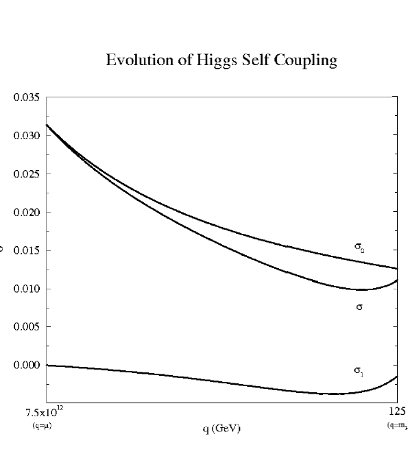
Figure 1: Evolution of the reduced Higgs Self Coupling $\sigma=\sigma_{0}+\sigma_{1}$ over the range from $m_{W}$ to $\mu=10^{14}$. The perturbation $\sigma_{1}$ remains small.

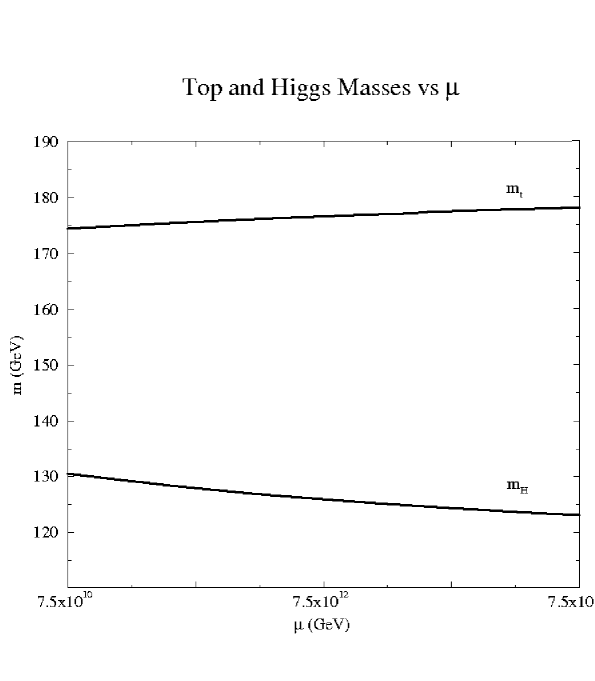
Figure 2: Variation of the top and Higgs masses with the matching scale $\mu$ over a range from $10^{10}$ to $10^{14}$ GeV. The scale $\mu=7.5\times 10^{12}$, for which $\sin^{2}(\theta(\mu))=\frac{3}{8}$, is defined as a ‘central value’.

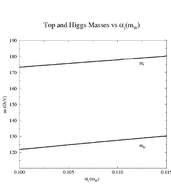
Figure 3: Variation of $m_{t}$ and $m_{H}$ with the strong coupling; $\alpha_{S}=0.107$ is considered the central value.

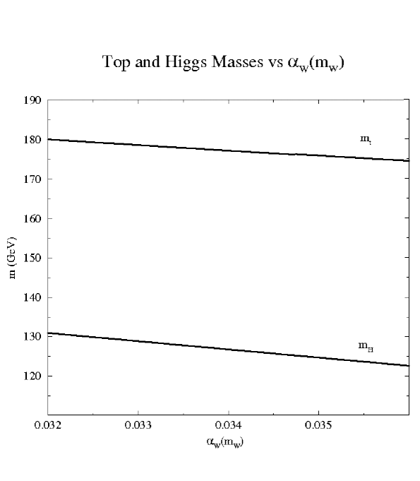
Figure 4: Variation of $m_{t}$ and $m_{H}$ with the weak coupling; $\alpha_{W}=0.0344$ is the central value.

References

- [1] Kahana D E and Kahana S H 1991 Phys. Rev. D43 2361–2368
- [2] Kahana D E and Kahana S H 1995 Phys. Rev. D52 3065–3071 (Preprint hep-ph/9312316)
- [3] Unal G (CDF) 1995 Nucl. Phys. Proc. Suppl. 39BC 343–347
- [4] Peryshkin A (D0 Collaboration) 1995 Nucl.Phys.Proc.Suppl. 39BC 353–356
- [5] Bjorken J 1963 Annals of Physics 24 174 – 187 ISSN 0003-4916 URL http://www.sciencedirect.com/science/article/pii/0003491663900691
- [6] Bardeen W A, Hill C T and Lindner M 1990 Phys. Rev. D 41(5) 1647–1660 URL http://link.aps.org/doi/10.1103/PhysRevD.41.1647
- [7] Terazawa H, Chikashige Y and Akama K 1977 Phys. Rev. D 15(2) 480–487 URL http://link.aps.org/doi/10.1103/PhysRevD.15.480
- [8] Eguchi T 1976 Phys. Rev. D 14(10) 2755–2763 URL http://link.aps.org/doi/10.1103/PhysRevD.14.2755
- [9] Nambu Y and Jona-Lasinio G 1961 Phys. Rev. 122(1) 345–358 URL http://link.aps.org/doi/10.1103/PhysRev.122.345
- [10] Bardeen J, Cooper L N and Schrieffer J R 1957 Phys. Rev. 108(5) 1175–1204 URL http://link.aps.org/doi/10.1103/PhysRev.108.1175
- [11] Kahana D 1989 Physics Letters B 229 9 – 15 ISSN 0370-2693 URL http://www.sciencedirect.com/science/article/pii/0370269389901457
- [12] Gross D J and Neveu A 1974 Phys. Rev. D 10(10) 3235–3253 URL http://link.aps.org/doi/10.1103/PhysRevD.10.3235
- [13] Marciano W J 1989 Phys. Rev. Lett. 62(24) 2793–2796 URL http://link.aps.org/doi/10.1103/PhysRevLett.62.2793
- [14] Marciano W J 1989 Phys. Rev. Lett. 62(24) 2793–2796 URL http://link.aps.org/doi/10.1103/PhysRevLett.62.2793
- [15] Gunion J 1990 The Higgs hunter’s guide Frontiers in physics (Addison-Wesley) ISBN 9780201509359 URL http://books.google.com/books?id=e8fvAAAAMAAJ
- [16] Buchmüller W and Love S 1982 Nuclear Physics B 204 213 – 224 ISSN 0550-3213 URL http://www.sciencedirect.com/science/article/pii/0550321382901456