Phase transition to two-peaks phase in an information cascade voting experiment

Abstract

Observational learning is an important information aggregation mechanism. However, it occasionally leads to a state in which an entire population chooses a sub-optimal option. When this occurs and whether it is a phase transition remain unanswered. To address these questions, we performed a voting experiment in which subjects answered a two-choice quiz sequentially with and without information about the prior subjects’ choices. The subjects who could copy others are called herders. We obtained a microscopic rule regarding how herders copy others. Varying the ratio of herders led to qualitative changes in the macroscopic behavior of about 50 subjects in the experiment. If the ratio is small, the sequence of choices rapidly converges to the correct one. As the ratio approaches 100%, convergence becomes extremely slow and information aggregation almost terminates. A simulation study of a stochastic model for $10^{6}$ subjects based on the herder’s microscopic rule showed a phase transition to the two-peaks phase, where the convergence completely terminates as the ratio exceeds some critical value.

I Introduction

The tendency to imitate others is one of the basic instinct of human. People effectively and inadvertently act as filters to provide the information that is most useful for an observer. Imitation and copying is a highly adaptive means of gaining knowledge Ren:2010 . It presumably results from an evolutionary adaptation that promoted survival over thousands of generations. It allows individuals to exploit the hard-won information of others Ren:2011 ; Ren:2010 . However, imitating or copying others has disadvantages. The acquired information might be outdated or misleading Ren:2011 ; Lor:2011 . Copying wrong information might lead to herding, where an entire population makes a wrong decision. This is referred to as information cascade or rational herding Bik:1992 ; Dev:1996 ; And:1997 ; Lee:1993 . Unfortunately, because imitation is a basic instinct and because it is economically rational to copy others, humans might not be able to evade such a catastrophic situation Bik:1992 . Social influences have many forms, including imitation, conformity and obedience Kel:1958 . Recent studies in cognitive neuroscience suggest that some type of imitation occurs automatically via the actions of “mirror neuron” systems Hey:2011 .

In the field of social psychology, many studies have focused on how humans use social information at the microscopic level Ren:2011 ; Gri:2006 . In the field of finance and economics, it is now widely believed that investors are influenced by the decisions of others and that this influence is a first-order effect Bik:1992 ; Dev:1996 . We now have a number of interesting models of rational herding based on simple, straightforward, and convincing intuition Bik:1992 ; Kir:1993 ; Dev:1996 ; Lux:1995 ; Con:2000 ; Cur:2006 ; Mor:2010 ; Gal:2008 ; Gon:2011 . Empirical financial research has focused on macroscopic data primarily because such data is easily available. Micro-macro aspects of information cascade have been studied in Goe:2007 . It was concluded that the information cascade is fragile and self-correcting. Even if the population makes a wrong decision at a point in the choice sequence, it will eventually turn to a correct choice. The analysis was based on a stochastic model, and the asymptotic behavior of the empirical choice sequences was not studied in detail. In order to study the nature of information cascade and, furthermore the possibility of phase transition, it is necessary to connect the micro-macro aspects without depending on a model assumption as far as possible. However, thus far, no empirical work has directly connected the microscopic and macroscopic aspects of information cascade and herding.

Two types of phase transitions have been predicted in a two-choice voting model depending on the strength of conformity of people His:2010 ; His:2011 . We set two types of individuals: herders and independents. The voting of independents is based on their fundamental values, while the voting of herders is based on the number of previous votes. If the herders are analog herders and they vote for each choice with probabilities that are proportional to the choices’ votes, there occurs a transition between the super and normal diffusion phases His:2010 . If the independents are the majority of voters, the voting rate converges at the same rate as in a binomial distribution, which is called the normal diffusion phase. As the proportion of herders is over 50%, the voting rate converges more slowwly than in a binomial distribution: this is called the super-diffusion phase. However, the presence of herders does not affect the accuracy of the majority’s choice. If the independents vote for the correct choice rather than for the wrong one, the majority of voters always choose the correct choice. The probability distribution of the voting rate has only one peak, and these two phases are collectively referred to as the one-peak phase. In the digital herder case, where herders always choose the choice with the majority of previous votes, the majority’s choice does not necessarily coincide with the correct choice, even if the independents vote for the correct choice rather than for the wrong one. When the fraction of herders increases, there occurs a phase transition, beyond which a state where most voters choose the correct choice coexists with one where most of them choose the wrong one His:2011 . If the fraction of herders is below the threshold value, most voters choose the correct choice and the system is in the one-peak phase. If the fraction is above the threshold value, the distribution of the voting rate has two peaks corresponding to the two coexisting states: this phase is called the two-peaks phase. We call the phase transition between the one-peak and two-peaks phases the information cascade transition.

In this paper, we have adopted an experimental and theoretical approach to the study of the phase transitions in information cascade . The organization of the paper is as follows. We explain the experimental design and procedure in section II. Section III is devoted to the analysis of the experimental data. We show that varying the ratio of herders led to qualitative changes in the asymptotic behavior of the convergence of the voting rate. In section IV, we introduce a stochastic model which simulates the system. We obtain a microscopic rule regarding how herders copy others. We performed a simulation study of a stochastic model for $10^{6}$ subjects based on the herder’s microscopic rule. The model showed the information cascade transition to the two-peaks phase, where the convergence completely terminates as the ratio exceeds some critical value. Section V is devoted to the conclusions. In the appendices, we explain the experimental setup in detail.

II Experimental design and procedure

Table 1: Experimental design.

Experiment	$T$	$\{r\}$	$M$	Subject pool	System
2010A	31	$\{0,1,2,3,5,7,9,\infty\}$	100	Kitasato Univ.	Face-to-Face
2010B	31	$\{0,1,2,3,5,7,9,\infty\}$	100	Kitasato Univ.	Face-to-Face
2011A	52	$\{0,1,5,11,21,\infty\}$	120	Hokkaido Univ.	Web
2011B	52	$\{0,1,5,11,21,\infty\}$	120	Hokkaido Univ.	Web

The experiments reported here were conducted at the Information Science Laboratory at Kitasato University in October 2010 and at the Group Experiment Laboratory of the Center for Experimental Research in Social Sciences at Hokkaido University between June 2011 and July 2011. The subjects included students from the two universities. We call the former experiment EXP2010 and the latter EXP2011. In EXP2010 (EXP2011), the number of individuals $T$ was 31 (52). We prepared two groups of subjects, group A and group B. In Total, 62 (104) subjects participated in EXP2010 (EXP2011). There were two sequences of subjects, and we denote the order of each subject by $t\in\{1,2,\cdots,T\}$. The number of questions $M$ in the two-choice quiz is 100 (120) in EXP2010 (EXP2011). Interaction between subjects in each group was permitted only through the social information given by the experimenter (Face-to-Face) in EXP2010 or by the experiment server (Web) in EXP2011. Table 1 summarizes the design.

The subjects answered the quiz individually with and without information about the previous subjects’ choices. This information, called social information, is given as the summary statistics of the previous $r$ subjects $\{C_{0}(r,t),C_{1}(r,t)\}$. We denote the $t+1$-th subject’s answer for case $r$ by $X(r,t+1)$, which takes the value 1 (0) if the choice is true (false). $\{C_{0}(r,t),C_{1}(r,t)\}$ are the numbers of subjects who choose each choice among the prior $r$ subjects as $C_{1}(r,t)=\sum_{t^{\prime}=t-r+1}^{t}X(r,t^{\prime})$ and $C_{0}(r,t)=r-C_{1}(r,t)$. The choice of $r$ is $r\in\{r\}=\{0,1,2,3,5,7,9,\infty\}(\{0,1,5,11,21,\infty\})$ in EXP2010 (EXP2011). Here, $r=0$ means that the subjects receive no information and must answer with their knowledge only. In the case $r=\infty$, the summary statistic is calculated from all previous subjects’ choices. The subjects answered the quiz with their knowledge only ($r=0$) initially. Next, they answered with $\{C_{0}(r,t),C_{1}(r,t)\}$ from $r=1$ to $r=\infty$ in increasing order of $r$ in the set $\{r\}$. Any differences between the choices in $r=0$ and $r\geq 1$ can be attributed to the social information.

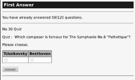
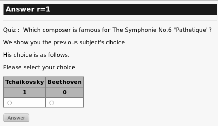
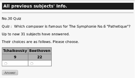
Figure 1: Snapshot of the screen for $r=0,1,$ and $\infty$ in EXP2011. The summary statistics $\{C_{0}(\infty,t),C_{1}(\infty,t)\}$ are given in the second row in the box in cases $r=1$ and $\infty$.

Fig. 1 shows the experience of the subjects in EXP2011 more concretely. The subjects entered the laboratory and sat in the partitioned spaces. After listening to a brief explanation about the experiment and the reward, they logged into the experiment web site using their IDs and started to answer the questions. A question was chosen by the experiment server and displayed on the monitor. First, subjects answered the question using their own knowledge only ($r=0$). Later, subjects received social information and answered the same question. Fig. 1 shows the cases $r=1$ and $r=\infty$. Subjects could then use or ignore the social information when making decisions.

II.1 Experimental procedure

We here explain in detail the procedure and the experience of the subjects in the experiment . A subject answered a question with no public information $(r=0)$ initially. The answer was denoted as $X(0,t)$ for the $t$-th subject in the subjects’ sequence. If the subject was first $(t=1)$, he answered only in the case $r=0$. $X(0,1)$ was copied to $X(r,1)$ as $X(r,1)=X(0,1)$ for $r\geq 1$ for later convenience. If $t>1$, the experimenter (in EXP2010) or the server (in EXP2011) calculated the social information $\{C_{0}(r,t),C_{1}(r,t)\}$ and gave it to the subject. If $t=2$, the subject answered the question in case $r=\infty$ with $\{C_{0}(\infty,1),C_{1}(\infty,1)\}$ and the answer was denoted as $X(\infty,2)$. Here, $C_{1}(\infty,1)$ is $X(0,1)$. By the convention $X(r,1)=X(0,1)$ for $r\geq 1$, we can write $C_{1}(\infty,1)=X(\infty,1)$. As $C_{1}(1,1)=C_{1}(\infty,1)$, we copy $X(\infty,2)$ to $X(1,2)$ as $X(1,2)=X(\infty,2)$. As in $t=1$, $X(1,2)=X(\infty,2)$ is copied to $X(r,2)$ as $X(r,2)=X(1,2)$ for $r>1$. If $t=3$, the subject answered the question in case $r=1$ with $\{C_{0}(1,2),C_{1}(1,2)\}$, and the answer was denoted as $X(1,3)$. The social information $\{C_{0}(1,2),C_{1}(1,2)\}$ was calculated with the answer $X(1,2)$ as $C_{1}(1,2)=X(1,2)$ by the copy convention $X(1,2)=X(\infty,2)$. Then, the subject answered in case $r=\infty$ and the answer was denoted as $X(\infty,3)$. $C_{1}(\infty,2)$ is $C_{1}(\infty,2)=X(0,1)+X(1,2)$, which can be written as $C_{1}(\infty,2)=X(\infty,1)+X(\infty,2)$. For $r>1$, $X(\infty,3)$ is copied to $X(r,3)$. By the copy convention, the social information in case $r$ can be expressed with the answers $\{X(r,t)\}$ in case $r$ only. If $t=4$, the subject answered the question in case $r=0$, which is written as $X(0,4)$, and then in case $r=1$, written as $X(1,4)$. Next, in EXP2011, the subject answered in case $r=\infty$, written as $X(\infty,4)$. The social information is $C_{1}(1,3)=X(1,3)$ and $C_{1}(\infty,3)=X(\infty,1)+X(\infty,2)+X(\infty,3)$. Fig. 2 gives the pictorial explanation of the procedure.

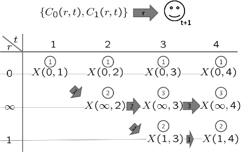
Figure 2: Pictorial explanation of experimental procedure. A subject answers the quiz questions in increasing order of $r$ from $r=0$ to $r=\infty$. The $t+1$-th subject answers in case $r$ with social information $\{C_{0}(r,t),C_{1}(r,t)\}$ and the answer is denoted as $X(r,t+1)$. The first subject $(t=1)$ answers only in the case $r=0$, which is written as $X(0,1)$. The second subject $(t=2)$ answers in the cases $r=0$ and $r=\infty$, which are written as $X(0,2)$ and $X(\infty,2)$, respectively. The third subject answers in case $r=0$, then in case $r=1$, and finally in case $r=\infty$; these are written as $X(0,3),X(1,3)$, and $X(\infty,3)$, respectively. The number in the circle indicates the order of the answer for each subject. The number in the arrow indicates the memory length of the social information. For $r=1$, it is one. For $r=\infty$, the $t$-th subject receives $t-1$ previous subjects’ information, and the length is $t-1$.

In general, if the order of the subject is $t$, there is no public information for $r>t-1$. There is the maximum value $r_{max}$ in the set $\{r\}$ that satisfies $r_{max}<t-1$. The subject answered from case $r=0$ to case $r_{max}$ in the set $\{r\}$ in increasing order of $r$. Then, the subject was given the social information from all priors ($r=\infty$) and answered in case $r=\infty$. He did not answer cases $r>r_{max}$ in the set $\{r\}$ and the answer in case $r=\infty$ was copied to the unanswered cases as $X(r,t)=X(\infty,t)$ for $r>r_{max}$ in set $\{r\}$. The answer in case $r$ started from the $r+2$-th subject in the sequence. For $t<r+2$, $X(r,t)=X(\infty,t)$ by the copy convention, and $\{C_{0}(r,t),C_{1}(r,t)\}$ can be written using only $\{X(r,t)\}$ as $C_{1}(r,t)=\sum_{t^{\prime}=t-r+1}^{t}X(r,t^{\prime})$ and $C_{0}(r,t)=r-C_{1}(r,t)$. We use the same conventions when we prepare a sequence of choices in case $r$. All sequences of choices $\{X(r,t)\}$ start from $t=1$. The percentage of correct answers up to the $t$-th subject is defined as $Z(r,t)=\sum_{t^{\prime}=1}^{t}X(r,t^{\prime})/t$, and the final value is $Z(r,T)$.

II.2 Quiz selection

Table 2: Five typical questions from the two-choice quiz in EXP2011. $q$ is the label of the questions in the quiz and $q\in\{0,1,2\cdots,119\}$.

q	Question	Choice0	Choice1	Answer
0	Which insect’s wings flap more in one minute?	mosquito	honeybee	0
1	During which period did the Tyrannosaurus Rex live?	Jurassic	Cretaceous	1
3	Which animal has a horn at birth?	rhinoceros	giraffe	1
7	Which is forbidden during TV programs in Korea?	commercials	kissing scenes	0
8	Which instrument is in the same group as the marimba ?	vibraphone	xylophone	1

We explain the choice of the questions in the quiz. In the experiment, it was necessary to control the difficulty of the questions. If a question is too easy, all subjects know the answer. If the question is too difficult, no subjects know the answer. In order to study social influence by varying the ratio of people who do not know the answer, it is necessary to choose moderately difficult questions. In EXP2010, we selected 100 questions for which only one among the five experimenters knew the answer. This choice means that the ratio is estimated to be around $80\%$ for the subjects. After EXP2010, we calculated $Z(0,T)$ for each question. In general, $Z(0,T)\geq 0.5$ for two-choice questions. A too-small value of $Z(0,T)$ indicates some bias in the given choices of the question. We excluded questions with too-small values of $Z(0,T)$ and prepared a new quiz with 120 questions in EXP2011. Table 2 shows five typical questions from EXP2011.

III Data analysis

In the analysis, the subjects are classified into two categories, independent and herder, for each question. If a subject knows the answer to a question with 100% confidence and the answer is not affected by others’ choices, he/she is categorized as independent. If the subject does not know the answer and if he/she may be affected by others’ choices, he/she is categorized as herder Mor:2010 ; His:2010 ; His:2011 . We assume that the probability of a correct choice for independent and herder subjects to be 100% and 50%, respectively. For a group with $p$ herders and $1-p$ independent subjects, the expectation value of $Z(0,T)$ is $E(Z(0,T))=1-p/2$. For each question in each group, we estimate $p$ by $p=2(1-Z(0,T))$ as the maximal likelihood estimate. The assumption of the random guess $(50\%)$ by the herder might be too simple. As $Z(0,T)$ approaches $0.5$ and almost all subjects do not know the answer to the question, $p$ approaches $100\%$ and the estimate works well.

Our experimental and analytical design has three advantages over both theoretical models and observational studies. (i) We control the amount of social information that the subjects receive by the change in $r$. This enables us to derive a microscopic rule for human decisions under social information Lat:1981 . (ii) Based on the answers in the absence of information ($r=0$), we can estimate the ratio of herders $p$, which will enable us to extract the herder’s decision rule from the results in (i). (iii) Our analysis focuses on the asymptotic behavior of the convergence of $Z(r,t)$ with fixed herder’s ratio $p$. We clearly see the collective behavior of humans and the qualitative change when $p$ is varied. In particular, we can study the possibility of the information cascade transition Lee:1993 ; His:2010 ; His:2011 ; Wat:2002 ; Cur:2006 .

We include a note about the controllability of $p$ in the experiment. In the experiment, after all $T$ subjects answered, we calculated $Z(0,T)$ and estimated the herder’s ratio $p$ as $p=2(1-Z(0,T))$. It may seem impossible to control $p$ in the experiment, but this is not so. We think $p$ is an inherent property of two-choice questions. If we can estimate $p$ for a large number of subjects $T>>1$, we can apply the same value to the experiments with other groups. We have compared the two values of $Z(0,T)$ of group A and B for the same question in EXP2011. Pearson’s correlation coefficient $\rho$ is 0.82, and there is a strong correlation. The system size $T$ in EXP2011 is very limited ($T\simeq 50$) and there remains some fluctuation in the estimation of $p$, but it will disappear for a large enough $T$. We can know $p$ in advance and control it in voting experiments.

III.1 Distribution of $Z(r,T)$

Table 3: Effect of social information on subjects’ decisions in (A) EXP2011 and (B) EXP2010. We divide the samples according to the size of $Z(r,T)$. $N(r)$ denotes the number of samples in each bin. $p_{avg}$ is estimated as the average value of $p=2(1-Z(0,T))$ in each bin. In the last column, the sub-optimal ratios are shown.

(A) EXP2011 No. $Z(r,T)[\%]$ $N(0)$ $p_{avg}[\%]$ $N(5)$ $N(\infty)$ Ratio 1 $<5$ 0 NA 0 2 NA 2 $5\sim 15$ 0 NA 4 18 NA 3 $15\sim 25$ 8 NA 8 22 8/8 4 $25\sim 35$ 16 NA 21 20 13/16 5 $35\sim 45$ 36 NA 24 8 28/36 6 $45\sim 55$ 43 96.7 26 9 16/43 7 $55\sim 65$ 46 79.3 34 10 9/46 8 $65\sim 75$ 45 62.7 40 14 2/45 9 $75\sim 85$ 33 41.9 45 33 0/33 10 $85\sim 95$ 11 21.3 32 67 0/11 11 $\geq 95$ 2 2.0 6 37 0/2 Total 240 240 240 76/240 (B) EXP2010 No. $Z(r,31)$ $N(0)$ $p_{avg}[\%]$ $N(5)$ $N(\infty)$ Ratio 1 $\leq 1/31$ 0 NA 0 3 NA 2 $2/31\sim 5/31$ 2 NA 7 20 2/2 3 $6/31\sim 9/31$ 6 NA 18 22 6/6 4 $10/31\sim 13/31$ 26 NA 21 14 23/26 5 $14/31\sim 17/31$ 52 97.6 33 6 26/52 6 $18/31\sim 21/31$ 54 74.6 21 7 5/54 7 $22/31\sim 25/31$ 33 49.1 35 29 1/33 8 $26/31\sim 29/31$ 25 26.3 47 67 0/25 9 $\geq 30/31$ 2 6.5 18 32 0/2 Total 200 200 200 63/200

There are $2\times 120(100)$ samples of sequences of choices for each $r$ in EXP2011 (EXP2010). We divide these samples into 11 (9) bins according to the size of $Z(r,T)$, as shown in Table 3A (3B). The samples in each bin share almost the same value of $p$. For example, in the sample in the No. 6 bin ($0.45<Z(0,T)\leq 0.55$) in EXP2011, there are almost only herders in the subjects’ sequence and $p\simeq 100\%$. 　On the other hand, in the sample in No. 11 bin ($Z(0,T)>0.95$), almost all subjects know the answer to the question and are independent $(p\simeq 0\%)$. An extremely small value of $Z(0,T)$ indicates some bias in the question. We omit data with $Z(0,T)<0.45(13/31)$ in the analysis of the system and we are left with 180 (166) samples in EXP2011 (EXP2010). The samples with $Z(0,T)<0.5$ in No. 6 bin in EXP2011 (No. 5 bin in EXP2010) have $p$ values larger than $100\%$. These values are errors of the estimation $p=2(1-Z(0,T))$. The standard deviation of $Z(0,T)$ is $p/2\sqrt{T}$ for fixed $p$. In the estimation of $p$, there is a fluctuation with the magnitude of order $\simeq p/\sqrt{T}$. If $p$ takes value larger than $100\%$, we take it to be $100\%$. Table 3 shows the number of data samples in each bin for $r=0,5$ and $r=\infty$ as $N(0),N(5),$ and $N(\infty)$. Social information causes remarkable changes in the subjects’ choices. For $r=0$ $(r=5)$, there is one peak at No. 7 (No. 9), and for $r=\infty$, there are peaks at No. 3 and No. 11 in EXP2011. Here, we compare the densities, not the value $N(r)$ itself. In the last column, we show the ratio of sub-optimal cases $\{Z(\infty,T)<1/2\}$ with respect to the $N(0)$ samples in each bin. The crucial problem is whether the sub-optimal cases $\{Z(\infty,T)<1/2\}$ remain so in the thermodynamic limit $T\to\infty$ Lee:1993 ; His:2011 .

Figure 3: Scatter plots of $Z(0,T)$ vs $Z(r,T)$ in EXP2011 for (A) $r=1$, (B) $r=5$, (C) $r=11$, (D) $r=21$ and (E) $r=\infty$. The vertical lines show the border of the bins in Table 3A.

In order to see the social influence more pictorially, we show the scatter plots of $Z(0,T)$ vs $Z(r,T)$ for all 240 samples in EXP2011 for each $r\in\{1(A),5(B),11(C),21(D),\infty(E)\}$ in Fig. 3. The $x$-axis shows $Z(0,T)$ and the y-axis shows $Z(r,T)$. The vertical lines show the boundary between the bins (from No. 1 to No. 11) in Table 3A. As we move from Fig. 3A $(r=1)$ to Fig. 3E $(r=\infty)$, the amount of social information $r$ increases. If the subjects’ answers are not affected by the social information, the data should distribute on the diagonal line. However, as the plots clearly indicate, this is not the case. As $r$ increases from $r=1$ to $r=\infty$, the changes $Z(r,T)-Z(0,T)$ increase and the samples scatter more widely in the plane. For the samples with $Z(0,T)\geq 0.75$ (Nos. 9, 10, 11 bins in Table 3A), the changes are almost positive and $Z(\infty,T)$ takes a value of about one. The sub-optimal ratios are zero in the bins. The average performance improves by the social information there. On the other hand, for the samples with $0.45\leq Z(0,T)<0.55$ (No. 6 bin in Table 3A), the social information does not necessarily improve the average performance. There are many samples with negative change $Z(\infty,T)-Z(0,T)<0$. These samples are in the sub-optimal state and constitute the lower peak in Table 3A.

III.2 Order parameters of the phase transition

We have seen drastic changes in the distribution of $Z(\infty,T)$ from the distribution of $Z(0,T)$. Table 3 shows the two-peaks structure in the distribution of $Z(\infty,T)$. In Fig. 3, we see an S-shaped curve in the case $r=\infty$. The natural question is whether these macroscopic changes can be attributed to the information cascade transition. In our previous work on the voting model with digital herders His:2011 , we showed the possibility of the phase transition from the one-peak phase to the two-peaks phase. If $p$ is smaller than some critical value $p_{c}$, the system is in the one-peak phase. The distribution of $Z(\infty,T)$ has only one peak at $Z(\infty,T)>1/2$. If $p>p_{c}$, the distribution of $Z(\infty,T)$ has two peaks at $Z(\infty,T)<1/2$ and $Z(\infty,T)>1/2$. In the thermodynamic limit $T\to\infty$, the probability that $Z(\infty,T)<1/2$ becomes a function of $p$, which is non-analytic at $p=p_{c}$ and takes a positive value for $p>p_{c}$. There are two candidates for the order parameter of the phase transition. One is the sub-optimal ratio $Z(\infty,T)<1/2$. The other is the variance of $Z(\infty,T)$, Var$(Z(\infty,T))$. Both candidates are zero for $p<p_{c}$ and positive for $p>p_{c}$ in the thermodynamic limit $T\to\infty$.

Figure 4: (A) The ratios of the sub-optimal $(Z(\infty,T)<1/2)$ cases, which are given in the last column of Table 3, and (B) the variance Var$(Z(\infty,T))$, are plotted vs $p$. The symbols $\circ(\triangle)$ indicate the results of EXP2011 (EXP2010).

Fig. 4 shows the plot of the two order parameters vs $p$. We plot (A) the ratios of the sub-optimal $(Z(\infty,T)<1/2)$ cases and (B) Var$(Z(\infty,T))$. The ratios are given in the last columns of Table 3. As $p$ increases, the order parameters change from zero to some finite value. They are monotonically increasing functions of $p$. However, in the behaviors, we cannot see any clear evidence of the phase transition. The system size is very small and we cannot see any non-analytic nature there. We cannot use them to prove the existence of the information cascade transition.

III.3 Asymptotic behavior of the convergence of $Z(\infty,t)$

We study the convergence of $Z(\infty,t)$ in the limit $t\to\infty$ to clarify the possibility of the information cascade transition. If information aggregation works under social information, $Z(\infty,t)$ converges to some value larger than half. The distribution of $Z(r,t)$ has only one peak: it is in the one-peak phase. Depending on the convergence behavior, the one-peak phase is classified into two phases. If the variance of $Z(r,t)$ shows normal diffusive behavior as $\mbox{Var}((Z(r,t))\propto t^{-1}$, it is called the normal diffusion phase. We note that the variance is estimated for the ratio, and the usual behavior $t^{1}$ for the sum of $t$ random variables is replaced by $\propto t/t^{2}=t^{-1}$. If the convergence is slow and it obeys $\mbox{Var}(Z(r,t))\propto t^{-\gamma}$ with $0<\gamma<1$, it is called the super diffusion phase Hod:2004 ; His:2010 . If information aggregation does not work and there is a finite probability that $Z(r,t)$ converges to some value less than half, the distribution of $Z(r,t)$ has two peaks Lee:1993 ; His:2011 . It is in the two-peaks phase, and $\mbox{Var}(Z(r,t))$ converges to some finite value in the limit $t\to\infty$.

Figure 5: Convergent behavior for (A) EXP2011 and (B) EXP2010. The convergence is given by the double logarithmic plot of $\mbox{Var}(Z(\infty,t))$ vs $t$ using the samples in the four bins for $r=0$ in Table 3A (No.6$(\circ)$,7$(\triangle)$,8$(\diamond)$ and 9$(\times)$) and in Table 3B (No.5$(\circ)$,6$(\triangle)$,7$(\diamond)$ and 8$(\times)$). The dotted lines are fitted results with $\propto t^{-\gamma}$ for $t\geq 20$.

Fig. 5A (B) shows the double logarithmic plots of $\mbox{Var}(Z(\infty,t))$ as a function of $t$ for EXP2011 (EXP2010). If the plot of Var$(Z(\infty,t))$ vs $t$ has a negative slope $(\gamma>0)$ in the limit $t\to\infty$, the system is in the one-peak phase. If the slope is zero $(\gamma\leq 0)$ in the limit $t\to\infty$, the system is in the two-peaks phase. We see that the convergence becomes very slow as $p$ increases. The exponent $\gamma$ is estimated by fitting with $\propto t^{-\gamma}$ for $t\geq 20$. It decreases from $1.43$ $(1.53)$ to $0.09$ with the increase in $p$ in EXP2011 (EXP2010). For the cases with $p=96.7\%(97.6\%)$ in EXP2011 (EXP2010), the system can be in the two-peaks phase.

IV Stochastic model and Simulation Study

The asymptotic analysis of the convergence of $Z(\infty,t)$ shows the possibility of the two-peaks phase in the cases $p=96.7\%$ and $97.6\%$. The negative slope $\gamma$ is remarkably small $(\sim 0.09)$ in both experiments. However, the system sizes are limited and far from the thermodynamic limit $T\to\infty$. In this section, we derive a microscopic rule as to how the herders copy others’ information. Based on the herder’s microscopic rule, we introduce an ad hoc stochastic model. A simulation study of the model for $10^{6}$ subjects showed the information cascade transition.

IV.1 Microscopic behavior of herders

We determine how a herder’s decision depends on social information. For this purpose, we need to subtract the independent subjects’ contribution from $X(r,t+1)$. The probability of being independent is $1-p$ and such a subject always chooses 1 ; the herder’s decision is then simply estimated as

$$(X(r,t+1)-(1-p)\cdot 1)/p.$$

The expectation value of this under $C_{1}(r,t)=n_{1}$ indicates the probability that a herder chooses an option under the influence of the prior $n_{1}$ subjects among $r$ choosing it. We denote it by $q_{h}(r,n_{1})$, and it is defined for $t\geq r$ as

$$q_{h}(r,n_{1})\equiv\mbox{E}((X(r,t+1)-(1-p))/p|C_{1}(r,t)=n_{1}).$$ (1)

The conditional expectation value in Eq.(1) is estimated using the samples that satisfy $C_{1}(r,t)=n_{1}$ from EXP2011. From the symmetry between $1\leftrightarrow 0$, we assume $q_{h}(r,n_{1})=1-q_{h}(r,r-n_{1})$. For $r=\infty$, the $t+1$-th subject obtains information from the previous $t$ subjects and $r$ is considered to be $t$. $r=\infty$ case is averaging several values of $r$. For $r=21$ and $\infty$, we study the dependence of $q_{h}(r,n_{1})$ on $n_{1}/r$ and round $n_{1}/r$ to the nearest values in $\{k/11|k\in\{0,1,2,\cdots,11\}\}$. In addition, we estimate $q_{h}(\infty,n_{1})$ for $t\geq 22$ to understand the herder’s decision under the largest amount of social information. The second reason is that the subjects receives much information for $t\geq 22$ and we can assume that the dependence of $q_{h}(\infty,n_{1})$ on $(t,n1)$ is replaced with the dependence on $n1/t$.

Figure 6: Microscopic rule of herder’s decision in EXP2011. It shows the probability $q_{h}(r,n_{1})$ that a herder chooses an option under the influence of the prior $n_{1}$ subjects among $r$ choosing it for cases $r=1(\times),5(\ast),11(\diamond)$ and $21(\triangle)$. For $r=\infty(\circ)$, $r$ is considered to be $t$. The thin solid curves are fitted results with Eq.(2) for $r=1,5,11,$ and $21$ from the bottom. The top thick solid line corresponds to $r=\infty$.

Figure 6 shows the plot of $q_{h}(r,n_{1})$ vs $n_{1}/r$. It is clear that $q_{h}(r,n_{1})$ is an almost monotonic increasing function of $n_{1}$. As $r$ increases, it shows stronger dependence on $n_{1}/r$, and the herder’s decision is affected more greatly by the prior subjects’ choices. We fit the plot by the following functional form:

$$q_{h}(r,n_{1})=\frac{1}{2}\left(a\tanh(\lambda_{r}(n_{1}/r-1/2))+1\right).$$ (2)

The parameters $a$ and $\lambda_{r}$ indicate the strength of the conformity of the subjects. Social psychology studies suggest that people’s likelihood to use social information depends on their mood Gri:2006 . $a$ denotes the net ratio of herders who react positively to the priors subjects’ choices. $\lambda_{r}$ denotes the strength of the dependence on social information. By the least squares fit, we obtain $a=0.761$ and $\lambda_{\infty}=3.80$ for $r=\infty$. The fitted result is also shown in Fig. 6. The values of $a$ and $\lambda_{\infty}$ depend on the experimental situation and on the system size $T$ . Using the same $a$, we fit the data for other $r$ using Eq.(2). The results are also given in Fig. 6. As the amount $r$ of social information increases, the strength of dependence $\lambda_{r}$ increases.

IV.2 Information cascade transition of voting model

To understand the behavior of the system in the thermodynamic limit $T\to\infty$, we simulate the system for large $T$ by a stochastic model based on Eq.(2). We introduce a stochastic process $\{X(t)\},t\in\{1,2,3,\cdots,T\}$. $X(t+1)\in\{0,1\}$ is a Bernoulli random variable and its probabilistic rule depends on all the previous $\{X(t^{\prime})\},t^{\prime}\in\{1,\cdots,t\}$ through $C_{1}(t)=\sum_{t^{\prime}=1}^{t}X(t^{\prime})$. The probability that $X(t+1)$ is 1 for $C_{1}(t)=n_{1}$, which is denoted as $q(t,n_{1})$, is given as

$$q(t,n_{1})=(1-p)+p\cdot\frac{1}{2}\left(a\tanh\lambda_{t}(n_{1}/t-1/2)+1\right).$$ (3)

We set $a$ as $a=0.761$ and $\lambda_{t}$ for $t\in\{1,5,11,21\}$ as $\lambda_{t}=\lambda_{r}$. Here, $\lambda_{r}$ takes the values given in Fig. 6. For other values of $t$ and $t<21$, we use the linearly extrapolated value. For $t>21$, we set $\lambda_{t}=\lambda_{\infty}$.

We denote the probability function Pr($\sum_{t^{\prime}=1}^{t}X(t^{\prime})=n)$ as $P(t,n)$. The master equation for $P(t,n)$ is

$$P(t+1,n)=q(t,n-1)\cdot P(t,n-1)+(1-q(t,n))\cdot P(t,n).$$ (4)

We solved the master equation recursively and obtain $P(t,n)$ for $t\leq 10^{6}$.

Figure 7: Plots of order parameters vs $p$ for the voting model and the limit $T\to\infty$. We plot (A) the sub-optimal ratio $Z(\infty,T)<1/2$ and (B) $\mbox{Var}(Z(\infty,T))$ vs $p$; here, $T$ is the length of the sequence. The symbol ($\circ$) indicates the experimental data for EXP2011$(r=\infty)$ ($T\simeq 50$) for the five bins No. 6, 7, 8, 9, and 10 in Table 3. The lines show the data from the stochastic model for $r=\infty$. For the stochastic model, we set $T=50$ (thick solid line), $10^{3}$ (thin solid), and $10^{6}$ (thick dotted). As $T$ increases, the non-zero regions of the order parameters move rightward. In the limit $T\to\infty$, the region reduces to $p>p_{c}=93.4\%$. The vertical chain line at $p=p_{c}$ shows the critical point of the phase transition between the one-peak phase $(p<p_{c})$ and the two-peaks phase $(p>p_{c})$.

Fig. 7 shows the results of the model. We plot (A) the sub-optimal ratio $Z(\infty,T)<1/2$ and (B) $\mbox{Var}(Z(\infty,T))$ vs $p$. For comparison, we plot the experimental results (EXP2011) using the symbol $\circ$. The model with $T=50$ well describes the experimental results quantitatively. In the figure, we also plot the results for $T=10^{3}$ and $10^{6}$. As $T$ increases, the non-zero regions of the order parameters move rightward. In particular, we see that there is a crossing point in the curves of Var$(Z(\infty,T))$ at $p=93.4\%$, which we denote as $p_{c}$. If $p<p_{c}$, $\mbox{Var}(Z(\infty,T))$ goes to zero as $T$ increases. On the other hand, if $p>p_{c}$, the variance seems to remain in the limit $T\to\infty$. This shows the phase transition between the one-peak and the two-peaks phases. For $p>p_{c}$, the system is in the two-peaks phase ($\gamma=0$). For $p<p_{c}$, the system is in the one-peak phase ($0<\gamma\leq 1$). In order to see the convergence rate (the exponent $\gamma$), it is necessary to study the asymptotic behavior of $\mbox{Var}(Z(\infty,t))$ for large values of $t$.

Figure 8: Thermodynamic limit and phase diagram. Asymptotic behavior of the convergence is given by the plot of $\gamma$ vs $p$. The symbols ($\circ$) show the $\gamma$s vs $p_{avg}$ in Fig. 5A. The lines show the results of the stochastic model with the system size $T=50$ (thick solid), $10^{3}$ (dotted), and $10^{6}$ (thick chain).

We estimate $\gamma$ from the slope of $\mbox{Var}(Z(t))$ as

$$\gamma=\log\frac{\mbox{Var}(Z(T-\Delta T))}{\mbox{Var}(Z(T))}/\log\frac{T}{T-\Delta T}$$ (5)

for the time horizons $T=50,10^{3}$ and $10^{6}$. For $T=50$, we take $\Delta T=30$ to match the analysis of the experimental data in EXP2011. For $T=10^{3}$ and $10^{6}$, we take $\Delta T=10^{2}$. The results are summarized in Fig. 8. For $T=50$, $\gamma$ is a monotonic decreasing function of $p$ and it describes the experimental results of EXP2011 well. For the limit $T\to\infty$, we compare the results with $T=50,10^{3}$, and $10^{6}$. $\gamma$ shows non-monotonic behavior as a function of $p$ for the latter two cases; it is an artifact of finite $T$. In the limit $T\to\infty$, $\gamma$ monotonically decreases from 1 to 0, and the threshold value is $p_{c}=93.4\%$ His:pre . For $p<p_{c}$ $(p>p_{c})$, the system is in the one-peak (two-peaks) phase.

V Conclusions

The instinct to imitate others led to the remarkably slow convergence of information aggregation as the herder’s ratio $p$ approached $100\%$. A stochastic model based on the herder’s microscopic copying rule predicted the information cascade transition between the one-peak ($p<p_{c}$) and the two-peaks phases ($p>p_{c}$) His:pre . In the one-peak phase, information aggregation works and the majority’s choice is always correct when the independents choose the correct choice rather than the incorrect one. In the two-peaks phase, the majority’s choice is not necessarily correct. The coexistence of the optimal $(Z(\infty,T)>1/2)$ and the sub-optimal $(Z(\infty,T)<1/2)$ states occurs there.

It has been thought that information cascade was fragile Dev:1996 ; And:1997 or self-correcting where the sub-optimal state disappears and switches to the optimal state Goe:2007 . Our study indicates that the system is in the two-peaks phase and that the sub-optimal state is stable against small perturbations for $p>p_{c}$ if the subjects are given the summary statistics $\{C_{0}(\infty,t),C_{1}(\infty,t)\}$. The conclusion might appear to be contradictory to the previous one, but this is not so. In the previous works, each subject has his own information and it is not necessary to follow the majority if one can trust his own information Goe:2007 . In addition, the social information is the time series of the previous choices $\{X(\infty,t^{\prime})\}_{1\leq t^{\prime}\leq t}$, and it contains much more information than the summary statistics $\{C_{0}(\infty,t),C_{1}(\infty,t)\}$. In our experiment, the herder does not have information and it is necessary to follow the majority if he wants to choose a correct answer. However, the system size in our experiment is very limited and it is difficult to infer the state of the system in the thermodynamic limit based only on experimental data. Our conclusion that there occurs a information cascade transition relies heavily on the results of the simulation study of the stochastic model. In addition, the experiments were performed with students at universities, and the scope of the subjects is thus very restricted. The robustness of the conclusion should be established by further experiments. For this purpose, a web-based experiment in artificial laboratories is promising Sal:2006 . There, we can approach the thermodynamic limit $T\to\infty$ more easily than in physical laboratories and study the micro-macro feature of information cascade.

Appendix A Experimental Setup

A.1 EXP2010

In EXP2010, the 62 subjects who participated in the experiment were recruited from the School of Science of Kitasato University. The subjects were randomly assigned to either group A or group B; each group had 31 subjects. In each session, one subject from each group entered the laboratory, a total of two subjects. We explained that we were studying how their choices were affected by the choices of others. After explaining the details of the experimental procedure and payment, each subject sat in front of an experimenter and had no contact with the other subject in the laboratory. The experiments on groups A and B were performed independently. Interaction between subjects in each group was permitted only through the social information given by the experimenter in front of each subject. The subjects were asked to answer the 100 questions in the two-choice quiz. The subjects answered the quiz with at most eight social influence conditions, including the case $r=0$. Each session lasted about one hour. In order to obtain data from all $T=31$ subjects in both groups, we performed the session 11 times on October 9 and and 10 times on October 16 and 23 in 2010. Subjects were paid upon being released from the session. There was a 2000 yen (about $24) participation fee and an additional 1000-yen reward (about $12) for the top ten subjects. The ranking of the subjects was calculated based on the ratio of correct answers to all questions and $r$.

A.2 EXP2011

In EXP2011, the 104 subjects who participated were recruited from the Literature Department of Hokkaido University. The subjects were randomly assigned to either group A or group B; each group had 52 subjects. In each session, between one and six subjects from each group entered the laboratory, for a total of between two and eleven subjects. The experiment was performed in the Group Experiment Laboratory of the Center for Experimental Research in Social Sciences of Hokkaido University. There were fifteen desks furnished with partitions and PCs. Each subject sat behind a partition and communication among them was prohibited. The experiments on groups A and B were performed independently. In order to study the effect of social information on the choices of the subjects, it was necessary to control the transmission of information from others in the same group. We developed a web-based voting system by which multiple subjects could simultaneously participate in the experiment. The subjects used a web browser to access the web voting server in the intranet. They could obtain information about the others’ choices from the summary statistics $\{C_{0}(r,t),C_{1}(r,t)\}$ shown on the monitor. Subjects did not know which questions the other subjects were answering or what their choices were.

With slides, we showed subjects how the experiment would proceed. We explained that we were studying how their choices were affected by the choices of others. In particular, we emphasized that the social information was realistic information calculated from the choices of previous subjects. The reason for this is that in contrast to EXP2010, the social information was given on the monitor and seemed less credible to the subjects. Through the slides, we also explained the payment. After the explanation, the experiment started. The subjects answered the 120-question quiz with at most six social influence conditions within about one hour. A total of 15 sessions were held on June 15 and 16 and from July 12 and 13 in 2011. Subjects were paid in cash upon being released from the session. There was a 600 yen (about $7) participation fee and additional rewards that were proportional to the number of correct answers. One correct choice was worth one point, and this was worth one yen (about one and a third cents).

Some subjects could not answer all the questions within the alloted time, so the number $T$ of subjects who answered a question varied. The distribution of $T$ is $\#\{T=52\}=143,\#\{T=51\}=5$, $\#\{T=50\}=2,\#\{T=49\}=85,\#\{T=48\}=4,\#\{T=47\}=1$. The average value of $T$ was $50.8$ and the standard deviation $\sigma_{T}$ was $1.48$. The average length of the sequence was about 50.

The assignment of quiz questions in EXP2011 was as follows. Each question has a label $q$ in $q\in\{0,1,2,\cdots,119\}$ and each subject has an ID number $i$. If the ID number $i$ of the subject was odd, the subject started with the question with the smallest $q$ in the pool not chosen by the server for another subject in the same group. If $i$ was even, the subject started with the question with the largest $q$ not chosen by the server for another subject. If another subject was answering a question, that question was never chosen by the server. It was strictly prohibited for multiple subjects to answer the same question simultaneously.

Appendix B Microscopic behavior of herders in EXP2010

Figure 9: Microscopic rule of herders’ decisions in EXP2010. It shows the probability $q_{h}(r,n_{1})$ that a herder chooses an option under the influence of the prior $n_{1}$ subjects among $r$ choosing it for cases $r=1(\times),3(\ast),5(\diamond)$ and $9(\triangle)$. For $r=\infty(\circ)$, the $t+1$-th subject’s decision depends on previous $t$ subjects’ decisions and $r$ is considered to be $t$. We estimate the dependences of $q_{h}(\infty,n_{1})$ on $n_{1}/t$ for $t\geq 10$, where $n_{1}/t$ is rounded to the nearest value in $\{k/9|k\in\{0,1,2,\cdots,9\}\}$. The solid curves are fitted results with $q_{h}(r,n_{1})=(a\tanh(\lambda_{r}(n_{1}/r-1/2))+1)/2$. For $r=\infty$ (the thick solid line), we set $r=t$. From bottom to top, the thin solid lines correspond to $r=1,3,5,$ and $9$.

We determine how a herder’s decision depends on social information in EXP2010. We follow the same procedure written in the main text. Fig. 9 plots the results. The fitted results with Eq.(2) are also shown. Compared with Fig. 6, the convergence to Eq.(2) is not so good. The system size $T=31$ is not enough to derive the microscopic rule.

Appendix C Estimate of $\gamma$ and its error bar

In our study, we focus on the asymptotic behavior of $\mbox{Var}(Z(\infty,t))$. In particular, we are interested in the power law behavior as $\mbox{Var}(Z(\infty,t))\propto t^{-\gamma}$. The negative slope $-\gamma$ of the double logarithmic plot of $\mbox{Var}(Z(\infty,t)$ vs $t$ gives the exponent $\gamma$ in the limit $t\to\infty$. In our analysis, we estimate $\gamma$ by the least squares fit with the functional form $a\cdot t^{-\gamma}$ in the range $20\leq t\leq T$. We denote the estimate as $\gamma_{exp}$.

For the error bar of the exponent $\gamma_{exp}$, we adopted the voting model to simulate the system and apply the parametric bootstrapping method based on it. First, we solved the model recursively up to $T=50-30$ and $T=50$ and obtained the probability functions $P(T,n)$ for both time horizons $T$. We defined $Z(T)$ as $Z(T)=\frac{n}{T}$ and estimated $\gamma$ by the relation

$$\gamma=\log\frac{\mbox{Var}(Z(T-\Delta T))}{\mbox{Var}(Z(T))}/\log\frac{T}{T-\Delta T}$$ (6)

using the probability function $P(T,n)$. Here, $\gamma$ was estimated in the range $T-\Delta T\leq t\leq T$. For $T=50$, we take $\Delta T=30$ to match the analysis of the experimental data in EXP2011. The estimate is exact, and we denote it as $\gamma_{exact}$. In EXP2011, the number of samples in each bin ranges from 33 to 46, and is very limited. We studied the stochastic model using the Monte Carlo method with the same sample size as the experimental data in each bin and estimated $\gamma$ for the samples. We repeated this $10^{4}$ times to obtain the samples of $\gamma$. Using the samples of $\gamma$, we estimated the 95% confidence interval, which is denoted as $[\gamma_{-},\gamma_{+}]$. The approximately estimated $\gamma$ was distributed around $\gamma_{exact}$. The upper (lower) deviation was calculated as $\Delta\gamma_{+}\equiv\gamma_{+}-\gamma_{exact}$ ($\Delta\gamma_{-}\equiv\gamma_{exact}-\gamma_{-}$). We estimated the 95% confidence interval of $\gamma_{exp}$ as $[\gamma_{exp}-\Delta\gamma_{-},\gamma_{exp}+\Delta\gamma_{+}]$. Using this procedure, we estimated the error bars for each $\gamma$ in Fig. 8.