We consider a topologically twisted version, recently introduced by Witten, of five-dimensional maximally supersymmetric Yang-Mills theory on a five-manifold of the form $M_{5}=\mathbb{R}\times W_{3}\times I$. If the length of the interval $I$ is sufficiently large, the supersymmetric localization equations admit pairs of static solutions (with the factor $\mathbb{R}$ interpreted as Euclidean time). However, these solutions disappear for a sufficiently short $I$, so by the topological invariance of the theory, they must be connected by an interpolating dynamic instanton solution. We study this for the case that $W_{3}$ is a three-sphere $S^{3}$ with the standard metric by making a spherically symmetric Ansatz for all fields. The solution is given as a power series in a parameter related to the length of $I$, and we give explicit expressions for the first non-trivial terms.

1 Introduction

On a five-manifold of the form

$$M_{5}=M_{4}\times I,$$ (1.1)

where $M_{4}$ is an oriented Riemannian four-manifold and $I$ is an interval, five-dimensional maximally supersymmetric Yang-Mills theory admits several inequivalent topological twistings. One of these was recently introduced by Witten [1] in an attempt to find a Yang-Mills interpretation of the Khovanov homology of knots [2]. This twisting corresponds to a homomorphism from the $\rm Spin(4)$ holonomy group of $M_{5}$ to the $\rm Spin(5)$ $R$-symmetry group of the Yang-Mills theory under which the spinor representation ${\bf 4}$ of $\rm Spin(5)$ decomposes as a direct sum ${\bf 2}+{\bf 2}$ of two chiral spinor representations of $\rm Spin(4)$. After such a twisting, the bosonic degrees of freedom can be described by fields on $M_{4}$ that in addition depend on a linear coordinate $y$ on $I$. These are the gauge connection $A$ with field strength $F$, a two-form $B$ which is self-dual with respect to the orientation and Riemannian structure of $M_{4}$, and a complex zero-form $\sigma$. The fields $F$, $B$, and $\sigma$ take their values in the vector bundle ${\rm ad}(E)$ associated to the gauge bundle $E$ via the adjoint representation of the gauge group $G$.

The path integral of this topological field theory localizes on supersymmetric field configurations that obey the elliptic set of equations [1]

$$F^{+}-\frac{1}{4}B\times B-\frac{1}{2}D_{y}B = 0$$ (1.2)

$$F_{y}+*DB = 0.$$ (1.3)

Here $*$ denotes the Hodge duality operator constructed from the orientation and Riemannian structure on $M_{4}$, $\times$ is an antisymmetric ‘cross-product’ on the rank three vector bundle $\Omega^{2,+}(M_{4})$ of self-dual two forms on $M_{4}$, $D$ is the gauge covariant exterior derivative on $M_{4}$, and $D_{y}$ is the covariant derivative with respect to the coordinate $y$ on $I$. Furthermore, we have decomposed the field strength $F$ (which is a two-form on $M_{5}$) as $F=F_{y}+F^{+}+F^{-}$, where the three terms are a one-form, a self-dual two-form and an anti-self-dual two-form on $M_{4}$ respectively. In addition to (1.2), supersymmetric field configurations obey some further equations that typically are equivalent to demanding that $\sigma$ vanish identically.

At the endpoints of $I$, the above bulk equations must be supplemented by suitable elliptic boundary conditions. (See the appendix of [3] for an accessible introduction to this concept.) Those that we will be using can be described as follows in terms of the Riemannian geometry of $M_{4}$ [1]: Suppose first that the gauge group $G$ is isomorphic to ${\rm SO}(3)$. As we approach a boundary component of $M_{5}$, the gauge connection $A$ tends to the Riemannian connection on the rank three vector bundle $\Omega^{2,+}(M_{4})$. The self-dual two-form $B$ has a simple pole at the boundary, the residue of which is given by the self-dual part of the second exterior power of the vierbein on $M_{4}$. (See [4] for a detailed discussion of a similar set of boundary conditions in four dimensions.) For a general gauge group $G$, the boundary behaviors of $A$ and $B$ are obtained in the same way, except that we have to identify ${\rm SO}(3)$ with a principally embedded subgroup of $G$ [5].

In this paper, we will only be concerned with the special case when

$$M_{4}=\mathbb{R}\times W_{3},$$ (1.4)

where the first factor can be interpreted as an Euclidean time direction and $W_{3}$ is a Riemannian three-manifold. We can then identify $B$ with a one-form $\phi$ on $W_{3}$ with values in ${\rm ad}(E)$. It is convenient to work in temporal gauge in which the time-component of the gauge field vanishes. We also single out the component of the gauge field in the direction of $I$ and denote this with $\chi$, (which can be regarded as a zero-form on $W_{3}$), so that $A$ and $F$ henceforth denote the components of the gauge field and its field strength in the directions of $W_{3}$ only. With $*$ and $D$ henceforth denoting the Hodge duality operator and the covariant exterior derivative respectively on $W_{3}$, the equations (1.2) then amount to

$$\frac{\partial A}{\partial t} = -*(F-\phi\wedge\phi)+D_{y}\phi$$ (1.5)

$$\frac{\partial\phi}{\partial t} = *D\phi-F_{y}$$ (1.6)

$$\frac{\partial\chi}{\partial t} = -*D(*\phi).$$ (1.7)

Static, i.e. $t$-independent, solutions to (1.5) are of particular importance. Imposing the additional gauge condition that the component $\chi$ of the gauge field in the direction of $I$ vanish, such solutions amount to configurations on $W_{3}\times I$ obeying the equations

$$\frac{\partial\phi}{\partial y} = *(F-\phi\wedge\phi)$$ (1.8)

$$\frac{\partial A}{\partial y} = *D\phi$$ (1.9)

$$*D(*\phi) = 0.$$ (1.10)

This can be interpreted as describing a perturbative ground state of the quantum theory on the spatial manifold $W_{3}\times I$. However, the energy of a bose-fermi pair of such states, i.e. a pair of solutions to the static equations (1.8), may become lifted by a non-perturbative tunneling effect represented by an interpolating solution to the dynamic equations (1.5) [1]. This phenomenon is well-known from applications of Morse theory to supersymmetric quantum mechanics [6] or, in an infinite dimensional setting, of Floer homology [7] to topological quantum field theory [8]. As usual, while the space of perturbative ground states may depend on the precise geometry of $W_{3}\times I$, the space of exact ground states is a topological invariant. In particular, with a fixed Riemannian structure on $W_{3}$ and a sufficiently short interval $I$, we would not expect the static equations (1.8) to have any solutions at all. So any solutions to (1.8) that may occur under particular circumstances should be pairwise connected by interpolating solutions to (1.5).

The aim of this note is to give an explicit example of such a tunneling solution. To this end, we will in the next section take $W_{3}=S^{3}$ with the standard metric, and make a spherically symmetric Ansatz for all fields. In section three, we will in this setting discuss the existence of a pair of solutions to the static equations (1.8) that were found in [4] provided that the interval $I$ has a length $\Delta y>2\pi$. For $\Delta y=2\pi$ the two solutions coalesce and they disappear for $\Delta y<2\pi$. These solutions can be approximated by a power series in a parameter $\varepsilon$ related to the interval length so that $\varepsilon=0$ for $\Delta y=2\pi$ and $\varepsilon\rightarrow\pm 1$ as $\Delta y\rightarrow\infty$. In section four, we will then discuss the corresponding approximate tunneling solution to (1.5), also as a power series in $\varepsilon$. We construct the first few terms explicitly and indicate how to proceed to arbitrary orders, although a rigorous proof of existence of the solution is still lacking.

While the present work is clearly concerned with a rather particular situation, it should be possible to generalize it in many different directions. In particular, one would hope that our results may be helpful for further developing the Yang-Mills interpretation [9] of the Jones polynomial [10] and Khovanov homology [2] of knot theory.

2 Spherical symmetry

To be able to find explicit solutions to the equations, we will henceforth specialize to the case that

$$W_{3}=S^{3}$$ (2.11)

with the standard metric. It is convenient to use the property that $S^{3}$ is isomorphic to the group manifold ${\rm SU}(2)$ and choose the dreibein $e$ as the Lie algebra valued Mauer-Cartan form obeying

$$de = -e\wedge e$$ (2.12)

$$= -*e.$$ (2.13)

The corresponding spin connection is then $\omega=\frac{1}{2}e$.

The most general spherically symmetric Ansatz for the gauge field $A$, the one-form $\phi$ and the zero-form $\chi$ (the component of the gauge field along $I$) is

$$A = \frac{1}{2}(1+u)e$$ (2.14)

$$\phi = se$$ (2.15)

$$\chi = 0,$$ (2.16)

where $u$ and $s$ are functions of time $t$ and the linear coordinate $y$ on $I$ only. The field $\chi$, which in general is a zero-form on $W_{3}$, is put to zero identically, since there is no non-vanishing possible spherically symmetric Ansatz for it. The last equation in (1.5) is then identically satisfied while the first two read

$$\frac{\partial u}{\partial t} = 2\frac{\partial s}{\partial y}-\frac{1}{2}u^{2}+2s^{2}+\frac{1}{2}$$ (2.17)

$$\frac{\partial s}{\partial t} = -\frac{1}{2}\frac{\partial u}{\partial y}+su.$$ (2.18)

The boundary conditions are that $u$ vanishes and that $s$ has simple poles with residues $\pm 1$ at the endpoints of the interval $I$.

The static equations (1.8) are of course obtained by requiring $u=\tilde{u}$ and $s=\tilde{s}$ to depend on $y$ only and read

$$\frac{d\tilde{u}}{dy} = 2\tilde{s}\tilde{u}$$ (2.19)

$$\frac{d\tilde{s}}{dy} = \frac{1}{4}\tilde{u}^{2}-\tilde{s}^{2}-\frac{1}{4}.$$ (2.20)

3 The static solutions

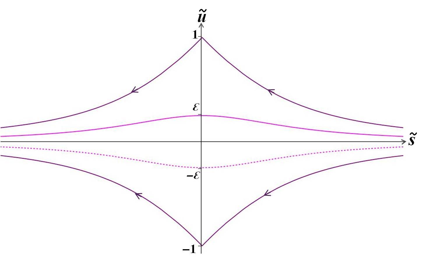
Figure 1: The flow in the $\tilde{s}-\tilde{u}$-plane, where arrows denote direction of increasing y. Only solutions in the interior of the space defined by the solutions flowing to or from the critical points $\tilde{s}=0$, $\tilde{u}=\pm 1$ will satisfy our boundary conditions. They appear in pairs related by reflection in the $\tilde{s}$-axis.

The static equations (2.19) can be visualized as a flow in the $\tilde{s}\tilde{u}$-plane, as is seen in figure 1 with arrows indicating the direction of increasing $y$. We have two critical points, namely $\tilde{s}=0,\tilde{u}=\pm 1$, which correspond to the trivial configurations $\phi=0,A=0$ and $\phi=0,A=e$ respectively. (The two critical points are in fact related to each other by a ‘large’ gauge transformation and are thus physically equivalent [4].) In the interior of the region bordered by the solutions flowing to and from these critical points, we have solutions that satisfy our boundary conditions. All solutions start at $\tilde{s}=\infty$, $\tilde{u}=0$ and end at $\tilde{s}=-\infty$, $\tilde{u}=0$ corresponding to the two boundary components of $W_{3}\times I$. The divergences of $\tilde{s}$ and the zeros of $\tilde{u}$ reflect the Nahm-poles of $\phi$ and the limits $\omega=\frac{1}{2}e$ of $A$ as we approach the boundaries.

We fix the symmetry under translations in $y$ by demanding that $\tilde{s}$ be an even function of $y$, from which it follows that $\tilde{u}$ is an odd function of $y$. The solutions can then be parametrized by a single integration constant which we take to be

$$\varepsilon=\tilde{u}(0)$$ (3.21)

with $-1<\varepsilon<1$. Clearly, the solutions appear in pairs related by reflection in the $s$-axis, i.e. $s\rightarrow s$ and $u\rightarrow-u$ so that $\varepsilon\rightarrow-\varepsilon$. A typical pair of such solutions has been indicated in figure 1.

The parameter $\varepsilon$ is related to the interval length $\Delta y$, which (provided that the functions $\tilde{u}$ and $\tilde{s}$ are known) can be computed as

$$\Delta y = \int dy$$ (3.22)

$$= \int_{\infty}^{-\infty}d\tilde{s}\Big{/}\frac{d\tilde{s}}{dy}$$ (3.23)

$$= \int_{\infty}^{-\infty}d\tilde{s}\Big{/}\left(\frac{1}{4}\tilde{u}^{2}-\tilde{s}^{2}-\frac{1}{4}\right).$$ (3.24)

The interval length is a monotonously increasing function of $\varepsilon^{2}$ with $\Delta y=2\pi$ for $\varepsilon=0$ and $\Delta y\rightarrow\infty$ as $\varepsilon\rightarrow\pm 1$.

This limit corresponds to solutions that approach one of the critical points as $y\rightarrow\infty$ (or $y\rightarrow-\infty$) and get stuck there; this means that the finite interval $I$ gets replaced by the half-line $\mathbb{R}^{+}$. This is actually the case that is most relevant for the study of knot theory [1]. It is also the only case in which we will have a non-zero instanton number. This can be seen as follows: The instanton density is locally a total derivative of the Chern-Simons invariants. The instanton number is thus given by considering the difference between them at the endpoints of the interval $I$. In cases where $I$ is finite, this will be trivially zero since the Chern-Simons invariants at the endpoints are equal. In the case where we have the entire half-line, our solutions interpolates between a trivial gauge field (at $y=\infty$) and a gauge field given by the spin connection on $S^{3}$ (at $y=0$). This results in an instanton number of $\pm 1$ for each of the critical points respectively.

For non-zero $\varepsilon$, it does not seem possible to find closed expressions for $\tilde{s}$ and $\tilde{u}$, but if we express them as odd and even power series respectively in $\varepsilon$

$$\tilde{s} = \tilde{s}_{0}+\varepsilon^{2}\tilde{s}_{2}+\ldots$$ (3.25)

$$\tilde{u} = \varepsilon\tilde{u}_{1}+\varepsilon^{3}\tilde{u}_{3}+\ldots,$$ (3.26)

the equations (2.19) amount to an infinite system of differential equations for the coefficients:

$$\frac{\partial\tilde{s}_{0}}{\partial y} = -\tilde{s}_{0}^{2}-\frac{1}{4}$$ (3.27)

$$\frac{\partial\tilde{u}_{1}}{\partial y} = 2\tilde{s}_{0}\tilde{u}_{1}$$ (3.28)

$$\frac{\partial\tilde{s}_{2}}{\partial y} = \frac{1}{4}\tilde{u}_{1}^{2}-2\tilde{s}_{0}\tilde{s}_{2}$$ (3.29)

$$\ldots$$ (3.30)

It is straightforward to solve these recursively: Together with the condition that $\tilde{s}$ be an odd function of $y$, the first equation yields

$$\tilde{s}_{0}=-\frac{1}{2}\tan\frac{y}{2}.$$ (3.31)

When this is inserted in the second equation, the solution is

$$\tilde{u}_{1}=\cos^{2}\frac{y}{2},$$ (3.32)

where the integration constant is fixed by the requirement that $\tilde{u}_{1}(0)=1$. The unique odd solution to the third equation is then

$$\tilde{s}_{2}=\frac{5y}{64}\cos^{-2}\frac{y}{2}+\sin\frac{y}{2}\left(\frac{5}{32}\cos^{-1}\frac{y}{2}+\frac{5}{48}\cos\frac{y}{2}+\frac{1}{12}\cos^{3}\frac{y}{2}\right).$$ (3.33)

This procedure can obviously be generalized to arbitrary orders in $\varepsilon$. We have also computed $\tilde{u}_{3}$ and $\tilde{s}_{4}$ explicitly, but the expressions are rather unilluminating and will be omitted here.

A general feature is that $\tilde{s}_{2n}$ will have poles of order $n+1$ and $\tilde{u}_{2n+1}$ will have poles of order $n-2$ at $y=\pm\pi$. (Poles of negative order are of course interpreted as zeros, so that $\tilde{u}_{1}$ has second order zeros as seen above, $\tilde{u}_{3}$ has first order zeros, and $\tilde{u}_{5}$ is regular and non-vanishing at $y=\pm\pi$.) This is related to the fact that $\tilde{u}$ and $\tilde{s}$ should vanish and have first order poles of unit residues respectively at the ends of the interval $I$. The length $\Delta y$ of $I$ depends on $\varepsilon$ in a way that dictates the singularity structure at $y=\pm\pi$ of the coefficients $\tilde{s}_{2n}$ and $\tilde{u}_{2n+1}$. To second order in $\varepsilon$ we have

$$\Delta y=2\pi+\varepsilon^{2}\frac{5\pi}{8}+{\cal O}(\varepsilon^{4}).$$ (3.34)

4 The tunneling solution

As described in the introduction, we expect the pair of solutions $\pm\tilde{u}$ and $\tilde{s}$ to the static equations (2.19) obtained for some fixed interval length $\Delta y>2\pi$, to be connected by an interpolating tunneling solution $u(y,\tau)$ and $s(y,\tau)$. The boundary conditions in the time direction are thus that

$$u(y,\tau)\rightarrow\pm\tilde{u}(y)$$ (4.35)

$$s(y,\tau)\rightarrow\tilde{s}(y)$$ (4.36)

as $\tau\rightarrow\pm\infty$. At the endpoints of the spatial interval $I$ for finite $\tau$, we require as before that $u$ vanishes and $s$ has simple poles with residues $\pm 1$. Here we have introduced a rescaled time variable $\tau$ as

$$\tau=\varepsilon t$$ (4.37)

in terms of which the equations (2.17) read

$$\varepsilon\frac{\partial u}{\partial\tau} = 2\frac{\partial s}{\partial y}-\frac{1}{2}u^{2}+2s^{2}+\frac{1}{2}$$ (4.38)

$$\varepsilon\frac{\partial s}{\partial\tau} = -\frac{1}{2}\frac{\partial u}{\partial y}+su.$$ (4.39)

In this way, it is consistent that $u$ and $s$ for fixed $y$ and $\tau$ be given by odd and even power series in $\varepsilon$ respectively:

$$s = s_{0}+\varepsilon^{2}s_{2}+\ldots$$ (4.40)

$$u = \varepsilon_{1}u_{1}+\varepsilon^{3}u_{3}+\ldots.$$ (4.41)

The equations (4.38) then amount to an infinite system of differential equations:

$$0 = 2\frac{\partial s_{0}}{\partial y}+2s_{0}^{2}+\frac{1}{2}$$ (4.42)

$$\frac{\partial s_{0}}{\partial\tau} = -\frac{1}{2}\frac{\partial u_{1}}{\partial y}+s_{0}u_{1}$$ (4.43)

$$\frac{\partial u_{1}}{\partial\tau} = 2\frac{\partial s_{2}}{\partial y}-\frac{1}{2}u_{1}^{2}+4s_{0}s_{2}$$ (4.44)

$$\ldots$$ (4.45)

Together with the condition that $s$ be an odd function of $y$, the first equation gives

$$s_{0}=-\frac{1}{2}\tan\frac{y}{2}.$$ (4.46)

When this is inserted in the second equation, we get a differential equation for $u_{1}$ as a function of $y$ (for fixed $\tau$) with the general solution

$$u_{1}=c_{1}(\tau)\cos^{2}\frac{y}{2}.$$ (4.47)

To determine the $\tau$-dependent integration constant $c_{1}$, we need to consider the third equation, which now reads

$$\frac{\partial c_{1}}{\partial\tau}\cos^{2}\frac{y}{2}=2\frac{\partial s_{2}}{\partial y}-\frac{1}{2}c_{1}^{2}\cos^{4}\frac{y}{2}-2s_{2}\tan\frac{y}{2}.$$ (4.48)

If this is regarded as an ordinary differential equation for $s_{2}$ as a function of $y$, the unique odd solution for an arbitrary function $c_{1}$ is

$$s_{2} = \frac{\partial c_{1}}{\partial\tau}\cos^{-2}\frac{y}{2}\left(\frac{3}{16}y+\sin\frac{y}{2}\left(\frac{3}{8}\cos\frac{y}{2}+\frac{1}{4}\cos^{3}\frac{y}{2}\right)\right)$$ (4.50)

$$+c_{1}^{2}\cos^{-2}\frac{y}{2}\left(\frac{5}{64}y+\sin\frac{y}{2}\left(\frac{5}{32}\cos\frac{y}{2}+\frac{5}{48}\cos^{3}\frac{y}{2}+\frac{1}{12}\cos^{5}\frac{y}{2}\right)\right).$$

The first and second term on each line gives rise to second order and first order poles at $y=\pm\pi$ respectively. These must agree with the poles in $\tilde{s}_{2}$ found in the previous section, which gives the condition

$$\frac{5}{64}=\frac{3}{16}\frac{\partial c_{1}}{\partial\tau}+\frac{5}{64}c_{1}^{2}.$$ (4.51)

Up to an inessential translation of the time-variable $\tau$, which we fix by requiring $c_{1}$ to be an odd function of $\tau$, the unique solution to this differential equation is $c_{1}=\tanh\frac{5\tau}{12}$ so that

$$u_{1}=\tanh\frac{5\tau}{12}\cos^{2}\frac{y}{2}.$$ (4.52)

As required for an interpolating solution, $u_{1}\rightarrow\pm\tilde{u}_{1}=\pm\cos^{2}\frac{y}{2}$ as $\tau\rightarrow\pm\infty$.

The corresponding solution (4.50) is best presented in the form

$$s_{2}=\tilde{s}_{2}+d_{2},$$ (4.53)

where the static term $\tilde{s}_{2}$ is given in (3.33) and the ‘dynamic’ term $d_{2}$ is given by the surprisingly simple result

$$d_{2}=-\frac{1}{12}\cosh^{-2}\frac{5\tau}{12}\sin\frac{y}{2}\cos^{3}\frac{y}{2}.$$ (4.54)

We note that not only is $d_{2}$ regular at $y=\pm\pi$ as required by the boundary conditions, but in fact it has third order zeros there. Moreover, as required for an interpolating solution, $d_{2}\rightarrow 0$ as $\tau\rightarrow\pm\infty$.

The generalization of this procedure to arbitrary orders in $\varepsilon$ is not as obvious as in the static case, but we believe that it can be carried out. A rigorous proof of this would be quite interesting. An outline is as follows: When the functions $s_{0},u_{1},\ldots,s_{2n}$ have been determined, the terms of order $2n+1$ and $2n+2$ in $\varepsilon$ respectively in equations (4.38) can be written as

$$\frac{\partial s_{2n}}{\partial\tau} = -\frac{1}{2}\frac{\partial u_{2n+1}}{\partial y}-\frac{1}{2}u_{2n+1}\tan\frac{y}{2}+\Bigl{[}(su)_{2n+1}-s_{0}u_{2n+1}\Bigr{]}$$ (4.55)

$$\frac{\partial u_{2n+1}}{\partial\tau} = 2\frac{\partial s_{2n+2}}{\partial y}-u_{2n+1}\tanh\frac{5\tau}{12}\cos^{2}\frac{y}{2}-2s_{2n+2}\tan\frac{y}{2}$$ (4.57)

$$+\left[-\frac{1}{2}(u^{2})_{2n+2}+u_{1}u_{2n+1}+2(s^{2})_{2n+2}-4s_{0}s_{2n+2}\right],$$

where we have used the expressions for $s_{0}$ and $u_{1}$ given above. It is important to note that the expressions in square brackets are given in terms of the previously determined functions $s_{0},u_{1},\ldots,s_{2n}$. The general solution to the first equation, regarded as an ordinary differential equation for $u_{2n+1}$ as a function of $y$ for fixed $\tau$, is

$$u_{2n+1}=2I_{2n+1}\cos^{2}\frac{y}{2},$$ (4.58)

where

$$I_{2n+1}=\int dy\cos^{-2}\frac{y}{2}\Bigl{[}(su)_{2n+1}-s_{0}u_{2n+1}-\frac{\partial s_{2n}}{\partial\tau}\Bigr{]}.$$ (4.59)

Clearly, the indefinite integral $I_{2n+1}$ is only determined up to an arbitrary ($\tau$-dependent) integration constant. We insert this result in the second equation, which then reads

$$2\frac{\partial I_{2n+1}}{\partial\tau}\cos^{2}\frac{y}{2} = 2\frac{\partial s_{2n+2}}{\partial y}-2I_{2n+1}(\tau)\tanh\frac{5\tau}{12}\cos^{4}\frac{y}{2}-2s_{2n+2}\tan\frac{y}{2}$$ (4.61)

$$+\left[-\frac{1}{2}(u^{2})_{2n+2}+u_{1}u_{2n+1}+2(s^{2})_{2n+2}-4s_{0}s_{2n+2}\right].$$

The solution to this equation, regarded as an ordinary differential equation for $s_{2n+2}$ as a function of $y$ for fixed $\tau$, is

$$s_{2n+2} = \cos^{-2}\frac{y}{2}\int dy\left\{\frac{\partial I_{2n+1}}{\partial\tau}\cos^{4}\frac{y}{2}+I_{2n+1}\tanh\frac{5\tau}{12}\cos^{6}\frac{y}{2}\right.$$ (4.63)

$$-\left.\frac{1}{2}\cos^{2}\frac{y}{2}\left[-\frac{1}{2}(u^{2})_{2n+2}+u_{1}u_{2n+1}+2(s^{2})_{2n+2}-4s_{0}s_{2n+2}\right]\right\}.$$

Imposing that $s_{2n+2}$ should be an odd function of $y$ determines the integration constant uniquely. The function $s_{2n+2}$ of course depends on $\tau$, and has poles at $y=\pm\pi$ of order up to $n+2$. But hopefully, it is of the form

$$s_{2n+2} = A_{2n+2}(\tau)\frac{\partial}{\partial y}\left(y\tan\frac{y}{2}\right)+\mathrm{static\;terms}+\mathrm{regular\;terms}$$ (4.64)

for some arbitrary (even) function $A_{2n+2}$ of $\tau$, i.e. the $\tau$-dependent part of $s_{2n+2}$ should have no poles beyond second order, and the first and second order poles should be given by the $y$-derivative of a first order pole. We believe that it should be possible to prove this property by a careful study of the structure of the singularities and time-dependence of the coefficients of $u$ and $s$. The unwanted $\tau$-dependent singular terms can now be removed by an appropriate choice of the integration constant in $I_{2n+1}$. Indeed, shifting

$$I_{2n+1}\rightarrow I_{2n+1}+C_{2n+1}(\tau)$$ (4.65)

gives shifts

$$u_{2n+1} \rightarrow u_{2n+1}+2C_{2n+1}\cos^{2}\frac{y}{2}$$ (4.66)

$$s_{2n+2} \rightarrow s_{2n+2}+\left(\frac{dC_{2n+1}}{d\tau}+\frac{5}{6}C_{2n+1}\tanh\frac{5\tau}{12}\right)\frac{3}{4}\frac{\partial}{\partial y}\left(y\tan\frac{y}{2}\right)$$ (4.69)

$$+\left(\frac{dC_{2n+1}}{d\tau}+\frac{5}{6}C_{2n+1}\tanh\frac{5\tau}{12}\right)\frac{1}{2}\sin\frac{y}{2}\cos\frac{y}{2}$$

$$+\frac{1}{3}C_{2n+1}\tanh\frac{5\tau}{12}\sin\frac{y}{2}\cos^{3}\frac{y}{2}.$$

The function $C_{2n+1}$ should thus be chosen to satisfy the ordinary differential equation

$$\frac{dC_{2n+1}}{d\tau}+\frac{5}{6}C_{2n+1}\tanh\frac{5\tau}{12}=-\frac{4}{3}A_{2n+2},$$ (4.70)

the solution of which is

$$C_{2n+1}=-\frac{4}{3}\cosh^{-2}\frac{5\tau}{12}\int d\tau A_{2n+2}\cosh^{2}\frac{5\tau}{12}$$ (4.71)

with the integration constant fixed by the requirement that $I_{2n+1}$ be an odd function of $\tau$. After this shift, the new function $s_{2n+2}$ will only have time independent singular terms, which of course should agree with the singularities of the static solution $\tilde{s}_{2n+2}$.

We have computed the functions $u_{3}$ and $s_{4}$ explicitly along these lines, but the resulting expressions are even less illuminating than in the static case and will be omitted here.

This research was supported by grants from the Göran Gustafsson foundation and the Swedish Research Council.

References

- [1] Witten, E. Fivebranes and Knots (2011). 1101.3216.
- [2] Khovanov, M. A Categorification Of The Jones Polynomial. Duke. Math. J. 101, 359–426 (2000).
- [3] Witten, E. A New Look At The Path Integral Of Quantum Mechanics (2010). 1009.6032.
- [4] Henningson, M. Boundary conditions for GL-twisted N=4 SYM (2011). 1106.3845.
- [5] Kostant, B. The principal three-dimensional subgroup and the betti numbers of a complex simple lie group. Am. J. Math. 81, 973–1032 (1959).
- [6] Witten, E. Supersymmetry and Morse theory. J.Diff.Geom. 17, 661–692 (1982).
- [7] Floer, A. Morse Theory For Lagrangian Intersections. J.Diff.Geom. 28, 523–547 (1988).
- [8] Witten, E. Topological Quantum Field Theory. Commun.Math.Phys. 117, 353 (1988).
- [9] Gaiotto, D. & Witten, E. Supersymmetric boundary conditions in super Yang-Mills theory. Journal of Statistical Physics 135, 789–855.
- [10] Jones, V. A polynomial invariant for knots via von Neumann algebras. Bull.Am.Math.Soc. 12, 103–111 (1985).