The Disordered Induced Interaction and the Phase Diagram of Cuprates

Abstract

There are processes in nature that resemble a true force but arise due to the minimization of the local energy. The most well-known case is the exchange interaction that leads to magnetic order in some materials. We discovered a new similar process occurring in connection with an electronic phase separation transition that leads to charge inhomogeneity in cuprate superconductors. The minimization of the local free energy, described here by the Cahn-Hilliard diffusion equation, drives the charges into regions of low and high densities. This motion leads to an effective potential with two-fold effect: creation of tiny isolated regions or micrograins, and two-body attraction, which promotes local or intra-grain superconducting pairing. Consequently, as in granular superconductors, the superconducting transition appears in two steps. First, with local intra-grain superconducting amplitudes and, at lower temperature, the superconducting phase or resistivity transition is attained by intergrain Josephson coupling. We show here that this approach reproduces the main features of the cuprates phase diagram, gives a clear interpretation to the pseudogap phase and yields the position dependent local density of states gap $\Delta(\vec{r})$ measured by tunnelling experiments.

1 Introduction

Almost 25 years of intense research on copper-oxide-based high-temperature superconductors has revealed many interesting and non-conventional results. It is impossible to explained all these data in detail by a single theory because some features may be sample dependent, but there are some general properties believed to be common to all cuprate superconductors like the pseudogap phase and the d-wave superconducting amplitude symmetry[1, 2, 3]. On materials which allow surface studies and thin films, mostly Bi, La and Y-based cuprates, there are well measured properties: the larger gap at the leading edge of the Fermi surface or antinodal (along the $Cu-O$ bonds) direction (($\pm\pi,0$) and ($0,\pm\pi$))[4], with the consequent nodal Fermi arcs above the critical temperature $T_{c}$[5, 6], and the spatially dependent local density of states gap $\Delta(\vec{r})$ measured by atomically resolved spectroscopy such as scanning tunneling microscopy (STM)[7, 8, 9, 10, 11, 12].

We show here that the fundamental superconducting interaction and some of these properties can be interpreted evoking an electronic phase separation (EPS) and its consequent temperature evolution of the charge inhomogeneity. There are many evidences that the charge distribution in the $CuO_{2}$ planes of the high temperature superconductors (HTSC) is microscopically inhomogeneous[13, 14]. Several different experiments like neutron diffraction[15, 16, 17], muon spin relaxation ($\mu SR$)[18, 19], nuclear quadrupole resonance (NQR) and nuclear magnetic resonance NMR[20, 21, 22] have detected varying local electronic densities. The spatial variations of the electronic gap amplitude $\Delta_{sc}(\vec{r})$ at a nanometer length scale[7, 8, 9, 10, 11, 12] may also be connected with the charge inhomogeneities. The origin of this electronic disorder is still not clear; it may be from the quenched disorder introduced by the dopant atoms[21, 23], or it may be due to competing orders in the $CuO_{2}$ planes[24]. Probably, the most convincing evidence of an EPS transition came from the increase of the local doping difference with decreasing temperature in the NQR experiment of Singer et al[20]. An EPS has been also used to interpret transport properties[25, 26] and to provide a clear interpretation to the non-vanishing magnetic susceptibility measured above the resistivity transition $T_{c}$[27, 28]. More recently a phase separation in $La_{2}CuO_{4+y}$ was analyzed after different times of the annealing processes[23]

The cuprates phase diagram has a crossover temperature or upper pseudogap detected by several transport experiments that merges with $T_{c}$ in the overdoped region[1, 2], i.e., for large dopant average level $p$. It is our fundamental assumption, and the starting point of our theory, that such crossover line is related to the EPS transition temperature $T_{PS}(p)$. Phase separation is a very general phenomenon in which a structurally and chemically homogeneous system shows instability toward a disordered composition[29]. However, the problem is to describe and to follow quantitatively the time and temperature evolution of the charge separation process. We have shown that an appropriate way to do this is through the general Cahn-Hilliard (CH) theory[30, 31, 32].

This approach uses an order parameter that is the difference between the temperature dependent local doping concentration $p(i,T)$ and the average doping level $p$, i.e., $u(i,T)\equiv(p(i,T)-p)/p$. Then the local Ginzburg-Landau (GL) free energy functional is,

$$f(i,T)={{{1\over 2}\varepsilon^{2}|\nabla u(i,T)|^{2}+V_{GL}(u(i,T))}}.$$ (1)

Where the potential ${\it V}_{GL}(u,i,T)=-A^{2}(T)u^{2}/2+B^{2}u^{4}/4+...$, $A^{2}(T)=\alpha(T_{PS}(p)-T)$, $\alpha$ and $B=1$ are temperature independent parameters. $\varepsilon$ gives the size of the grain boundaries among two distinct phases[31, 32].

The CH equation can be derived[29] from a continuity equation of the local free energy $f(i,T)$, $\partial_{t}u=-{\bf\nabla.J}$, with the current ${\bf J}=M{\bf\nabla}(\delta f/\delta u)$, where $M$ is the mobility or the charge transport coefficient, normally incorporated in the time step intervals. Therefore,

$$\frac{\partial u}{\partial t}=-M\nabla^{2}(\varepsilon^{2}\nabla^{2}u+{\it V}_{GL}(p,i,T)).$$ (2)

We have already made a detailed study of the CH differential equation by finite difference methods[31] which yields the density profile $u(p,i,T)$ in a $105\times 105$ array as function of the time steps, up to the stabilization of the local densities[32, 33, 34, 35, 36]. Here we study the EPS profile as the parameter $A$ changes from $A=0$ near $T=T_{PS}$ to $A=1$ close to $T=0$K.

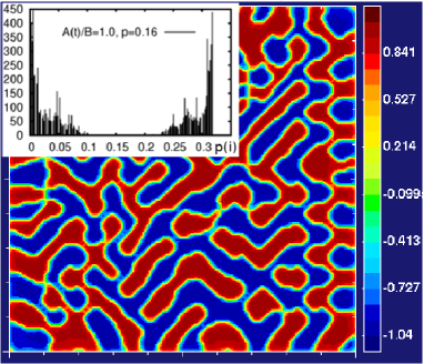
Figure 1: (color online) The order parameter $u(i)\equiv(p(i)-p)/p$ simulation of the inhomogeneous local charge density on a $100\times 100$ sites. In the inset, the local densities $p(i)$ histogram of the optimal compound ($p=0.16$) indicating the tendency to segregate into grains with $p(i)\approx 0$ and $p(i)\approx 0.32$. As the temperature $T$ goes down below the phase separation temperature $T_{ps}$ the segregation increases.

In Fig.(1) we show a typical density profile after a long time evolution ($A,B=1$ and average doping $p=0.16$) with a high segregation level as it is seen by the local densities histogram (in the inset). The colour map shows regions with $p(i)\approx 0$ (red) and $p(i)\approx 2p$ (blue). The lack of direct measurements does not let us know whether all cuprates have such high level of charge inhomogeneity and it is possible that it varies according to a specific family of compounds.

2 The EPS and the Fundamental Interaction

During the EPS process the holes move preferable along the $Cu-O$ bonds or nearest neighbor hopping according to the measured dispersion relations[37]. Here we show by the local free energy calculations that this hole motion can be regarded as if it was produced by an effective hole-hole interaction as has been proposed before, like, for instance, by the work of Trugman[38]. To see this we perform numerical simulations of the local potential energy $V_{GL}(u(i,T))$ with the solutions $u(i,T)$ of the CH equation. The results are shown in Fig.(2) and they reveal two important and different effects: i- it divides the system in many tiny potential wells as it is shown on the free energy map of Fig.(2). The inset shows also the free energy along the white straight line on 42 sites ($\approx 160\AA$) showing these potential wells and the barriers between the low and high density regions. We define the height of these inter-grain or grain-boundary potential $V_{gb}$ since it gives a granular structure to the system. In this way each small grain of low or high density is a small bounded region by $V_{gb}$. Each of these potential wells form local single-particle bound states. These bound states are seen experimentally by the local density of states (LDOS) derived from STM experiments[7, 8, 9, 10, 11, 12]. $V_{gb}(T)$ is function of the temperature and increases when the temperature goes down below $T_{PS}$ as it is demonstrated by the two insets in Fig.(2) taken from simulations at two different temperatures.
ii- Second, in the process of minimizing the local free energy, the holes move to cluster themselves in a similar fashion as if they attract themselves, forming the hole rich and hole poor regions.

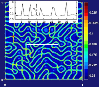
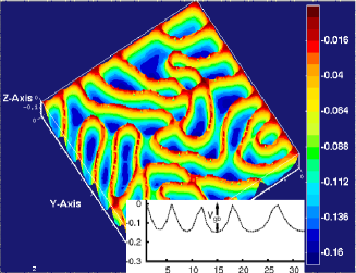
Figure 2: (color online) On the top panel, the potential ${\it V}(p,i,T)$ planar map simulation. The values on 42 sites at the white line are shown in the top inset to demonstrate the potential wells with average barrier $\approx V_{gb}$ where single-particle bound states appear. The lower panel is a 3-dimensional section of the above map, where the potential barriers are more clearly visible, at a higher temperature and smaller $V_{gb}$, as shown in the inset.

This hole-hole effective attraction is schematically illustrated in Fig.(3) where a) represents a homogeneous system with $p=0.25$ (one hole at each four sites) and b) the motion toward clusters formation of low ($p_{i}=0$) and high densities ($p_{i}=2p=0.50$). This hole movement can be regarded as originated from an effective two-body attraction. Conceptually, this is similar to the spin-spin exchange interaction, that arises from the Pauli principle and the minimization of the local electronic energy, that produces ferromagnetic order.

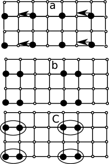
Figure 3: Schematic representation of the cluster and pair formation. a) represents a homogeneous system with $p=0.25$ (one hole at each four sites) and the CH phase separation produces hopping preferably along the $Cu-O$ bond toward clusters formation of low ($p_{i}=0$) and high densities ($p_{i}=0.50$)(b). At low temperatures, d-wave superconducting pairs may be formed (c).

We made simulations using ${\it V_{GL}}(p,i,T)$ at low temperatures up to $T_{PS}(p)$, where the disorder disappears. The low temperatures values are parameterized to yield the low temperature gaps at different average doping $p$ from the STM measurements of the series of Bi2212 LDOS[7]. In this way we obtain a numerical estimate of $V_{gb}(p,T)$ that reproduces the STM results of this entire family. Namely

$$V_{gb}(p,T)=V(p)V(T)=(-0.7+2.4p)(1-(T/T_{PS})^{1.5}),$$ (3)

where the values are in $eV$, $V(p)$ is linear and vanishes at $p\approx 0.32$ following the approximate behavior of $T_{PS}(p)$ from the $T_{0}(p)$ curve plotted in the phase diagram of Timusk and Statt[1]. The power to the 1.5 temperature dependence is taken from the work of Cahn and Hilliard[30].

3 BdG-CH Combined Calculations

We now perform self consistent-calculations with the Bogoliubov-deGennes (BdG) theory in the system. There are some possibilities to obtain a solution with a disordered density and local dependent superconducting gaps, for instance: Ghosal et al[39] introduced a varying impurity potential in the chemical potential to assure the local changes in the hole density. Other approach is to introduce modulations to the superconducting pair interaction due to the out of plane dopant atoms[40]. Here we introduce a third method, different but it contains the spirit of the work of Ghosal: we keep the local disordered density solution derived from the CH simulation fixed at all points and determine self-consistently the respective local chemical potential and d-wave superconducting amplitudes. In this way we capture the phase separation solution like that shown in Fig.(1). To calculate the superconducting amplitudes and single-particle excitations and bound states we used the effective hole attraction $V_{gb}$ in the form of a local two-body nearest neighbor attraction. Although the potential is constant in space, the different local densities yield different superconducting amplitudes. Starting with an extended Hubbard Hamiltonian with nearest neighbor hopping $t=0.15$eV and next nearest neighbor hopping of $t_{1}/t=-0.64$, close to the ARPES value of $t_{1}/t=-0.50$[37], the BdG mean-field equations are written in terms of the BdG matrix[32, 33, 34, 35, 36]:

These equations, defined in detail in Refs.[32, 34], are solved self-consistently for $E_{n}\geq 0$ together with the eigenvectors $(u_{n},v_{n})$ and d-wave pairing amplitudes

$$\Delta_{d}({\bf x}_{i}) = -{V_{gb}\over 2}\sum_{n}[u_{n}({\bf x}_{i})v_{n}^{*}({\bf x}_{i}+{\bf\delta})+v_{n}^{*}({\bf x}_{i})u_{n}({\bf x}_{i}$$ (4)

$$+{\bf\delta})]\tanh{E_{n}\over 2k_{B}T},$$

and the input inhomogeneous hole density is given by

$$p({\bf x}_{i})=1-2\sum_{n}[|u_{n}({\bf x}_{i})|^{2}f_{n}+|v_{n}({\bf x}_{i})|^{2}(1-f_{n})],$$ (5)

and converges self-consistently to a $N\times N$ square (here we made calculations with $N=28-42$) in the CH density map of Fig.(1). $f_{n}$ is the Fermi function. $V_{gb}$ is maintained fixed at each temperature $T$ and for a given compound with average doping $p$.

The BdG-CH combined calculations yield larger superconducting amplitudes $\Delta_{d}(i,p,T)$ in the high density grains and smaller amplitudes at regions with low densities. The variations on $\Delta_{d}(i,p)$ are usually $\pm 12\%$ around the average value $\Delta^{av}_{d}(T,p)\equiv\sum_{i}^{N}\Delta_{d}(T,i,p)/N$. However, due to the mean-field approach, all the amplitudes vanishes at the same temperature $T^{*}(p)$. We believe that a more rigorous treatment would yield that larger gaps vanish at larger temperatures, but there are many interesting consequences even within this simple approach. Due to the functional form of $V_{gb}(p)$ in Eq.(3) the $\Delta^{av}_{d}(T,p)$ decreases systematically with $p$ as it is shown in Fig.(4). As the temperature decreases below $T^{*}(p)$ the grains become superconductors but the grain boundary potential barrier $V_{gb}$ prevents the current to flow freely. Thus, the electronic grain structure of cuprate superconductors at low temperatures can be regard as formed by numerous $S_{i}-I-S_{j}$ junctions.

Consequently, we apply the theory of granular superconductors[41] to these tiny electronic grains, and as an approximation, we use the Josephson coupling expression to an $S-I-S$ junction given by[41].

$$E_{J}(p,T)=\frac{\pi h\Delta(T,p)}{4e^{2}R_{n}}tanh(\frac{\Delta(T,p)}{2K_{B}T_{c}}).$$ (6)

$\Delta^{av}_{d}(T,p)$ is the average of the calculated BdG superconducting gaps $\Delta_{d}(i,T)$ on the entire $N\times N(N=28-42)$ square. The $R_{n}$ is the normal resistance of a given compound, which we take as proportional to the $\rho_{ab}$ measurements[42] on the complete series of $La_{2-p}Sr_{p}CuO_{2}$. The values of $\Delta^{av}_{d}(T,p)$ as function of $p$ are plotted in the top panel of Fig.(4). In the low panel we plot the two sides of Eq.6) and the intersections yield one of our main result: the $T_{c}(p)$ dome shape in agreement with the Bi2212 series.

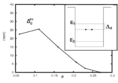
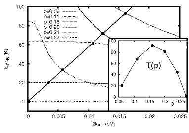
Figure 4: In the top panel we plot the average $\Delta_{d}(T,p)$ and in the inset the schematic single particle energies that appear in the LDOS. In the low panel, the Josephson coupling among superconducting grains $E_{J}(p,T)$ for some selected doping values as function of T and $k_{B}T$. The curves intersections give the dome shape $T_{c}(p)$, as plotted in the inset.

The zero resistivity transition takes place when the Josephson coupling $E_{J}$ among these tiny grains is sufficiently large to overcome thermal fluctuations[43], i.e., $E_{J}(p,T=T_{c})\approx k_{B}T_{c}(p)$, what leads to phase locking and long range phase coherence. Consequently the superconducting transition in cuprates occurs in two steps, similar to a superconducting material embedded in a non superconducting matrix[43]: First, as the temperature goes down, by the appearing of intragrain superconductivity (pseudogap phase) and by Josephson coupling with phase locking (superconducting phase). We emphasize that the reason for the dome shape form of $T_{c}(p)$, with the optimum value near $p=0.16$, is due to the fact that $\Delta^{av}_{d}(T,p)$ decreases and $(1/R_{n}$) increases with $p$.

4 The STM Results and Interpretation

One of the most important experimental result without a widely accepted explanation is the spatial dependent energy gaps $\Delta(\vec{r})$ measured by Scanning Tunneling Microscopy (STM)[7, 8, 9, 10, 11, 12]. We show here that this behavior can be reproduced by the microscopic granular theory developed above. We perform calculations on the non-uniform charge system but the usual local density of states (LDOS)[44] at different places ${\bf x}_{i}$ are not so sharp and difficult to get their real value. To improve the determination of the peaks positions, although the measured LDOS of cuprates are not symmetric, we deal with the following symmetric LDOS,

$$N_{i}(E)=\sum_{n} [ |u_{n}({\bf x}_{i})|^{2}+|v_{n}({\bf x}_{i})|^{2}]\times$$ (7)

$$[f_{n}^{{}^{\prime}}(E-E_{n})+f_{n}^{{}^{\prime}}(E+E_{n})].$$

$f_{n}$ is the Fermi function, the prime is the derivative with respect to the argument, and $u_{n},v_{n}$ and $E_{n}$ are respectively the eigenvectors and positive eigenvalues (quasi-particles exciting energy) of the BdG matrix equation[32, 33, 34, 35, 36].

To study the effects of the disordered density, we examine the ratio $LDOS(V_{gb}\neq 0)/LDOS(V_{gb}=0)$. $LDOS(V_{gb}=0)$ contains the inhomogeneous charge distribution and $LDOS(V_{gb}\neq 0)$, the unnormalized local density of states, vanishes around the Fermi energy due to the superconducting gap and the single particle levels in the grains. This LDOS ratio yields well-defined peaks and converges to the unity at large bias, in close agreement to similar approach of the LDOS ratios calculated from STM measurements[9].

These features are illustrated in Fig.(5) for an overdoped $p=0.20$ compound near a grain boundary at a representative average doping hole point. At $T=40$K, $V_{gb}=0.240$eV and for large applied potential difference ($V>0.1$eV) both LDOS, $LDOS(V_{gb}\neq 0)$ and $LDOS(V_{gb}=0)$ converge to the same values, but around zero bias ($V\approx 0$) there is a large spectral weight suppression in $LDOS(V_{gb}$ only. This is due to the single-particle bound states and to the superconducting pair formations and both effects are destroyed as the temperature is raised, according to the lower panel of Fig.(6). To distinguish clearly the effect of the superconducting gap in the DOS of Fig.(5) we draw arrows at the $\Delta_{d}$ values. Notice that it appears only as an anomaly in the LDOS curve with two well-defined peaks, as it was reported by some STM data[10, 11]. Consequently, the gap calculated directly from the LDOS peaks is identified with the with the pseudogap $\Delta_{PG}(p)$. This also implies that STM may not measure the local superconducting gap but, in some cases, the local gap from the single particle bound states formed in the isolated islands.

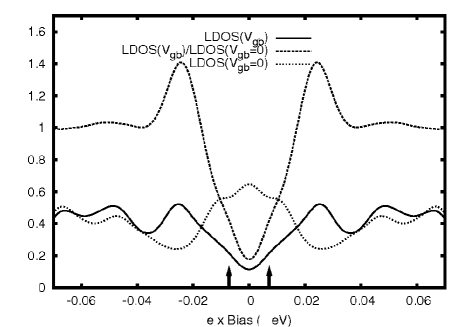
Figure 5: The real LDOS with $V_{gb}=0.240$eV, the zero pair potential LDOS $V_{gb}=0$ and the normalized LDOS on an overdoped $p=0.20$ sample for $V_{gb}=0.240$eV. The zero pair potential LDOS $V_{gb}=0$ is also shown. The arrows show the values of the local superconducting gap $\Delta_{d}=7.2meV$, smaller than the LDOS gap ($\approx 24$meV).

In Fig.(6) we plot the calculated low temperature LDOS at four representative locations with different densities of the $p=0.16$ optimum compound. We see that the peaks vary from $35-65meV$ in accordance with the data of McElroy et al[7]. This overall agreement comes from the choice of the parameter in the potential $V_{gb}$ (Eq.3), however the local variations in nanometer scale comes from the charge inhomogeneity calculated from the CH approach and also reproduces the it local variations of the STM LDOS[7]. The temperature evolution in the low panel of Fig.(6) shows that the single-particle or LDOS gap closes near $T^{*}=115$K, more than 20K above $T_{c}$.

Figure 6: In the top panel, the LDOS at four different regions with local doping $n_{i}$. At the low panel the temperature evolution of the LDOS just to the closing of the gap at $T\approx 114$K, above $T_{c}\approx 92$K. The arrows show the average $\Delta^{av}_{d}(T=40K)=15meV$. In low panel we show the LDOS temperature evolution at one region ($p_{i}=0.25$). The kink at low bias in the low temperature curve has also been observed by many STM data[8, 9, 10, 11, 12] and in our calculations it is due to the superconducting gap $\Delta_{d}(T=40K)=21meV$.

The calculations in the density disordered system yield that the low temperature superconducting gaps $\Delta_{d}(i,p=0.16)$ vary from $7-23meV$, depending on the local density, that is, they are much smaller than the gaps derived from the LDOS peaks shown in Fig.(6). Consequently we conclude that the measured LDOS gaps are due to the single-particle bound states gaps $\Delta_{PG}(i,p,T)$ that leads to the following scenario to the cuprate superconductors: The pseudogap phase derived from our calculations is formed due to the granular behavior by the single-particle bound states gaps $\Delta_{PG}(i,p,T)$ in the isolated local doping dependent regions or grains. Like in granular superconductors, there are also the intragrain superconducting amplitude $\Delta_{d}(i,p,T)$. At lower temperatures the superconducting phase also contains both gaps but has phase coherent through the Josephson coupling among the grains. At the overdoped region $T^{*}(p)$ approaches $T_{c}(p)$ while their difference increases in the underdoped region. These two calculated curves as function of $p$ are shown in the phase diagram of Fig.(7).

We have also plotted the EPS line $T_{PS}(p)$ used in our calculations where stats the phase separation process and which we assumed to be near the observed anomaly calledupper-pseudogap Timusk and Statt[1]. As mentioned in the introduction, this transition may be due to the presence of the AF order which has lower free energy[24] (intrinsic origin) or due to out of plane arrangements of dopant atoms[21, 22, 23] (extrinsic origin).

Figure 7: The calculated phase diagram of cuprate superconductors as derived from the EPS transition $T_{PS}(p)$ and the formation of tiny grains. The onset of single particle bound states and superconducting amplitude formation occurs at $T^{*}(p)$. The dome shape $T_{c}(p)$ curve is due to Josephson coupling among the grains. These three lines are in agreement with the experimental results.

5 Conclusions

The main ideas of our work come from the application of the CH theory to model the highly non-uniform charge distribution in cuprates. This approach describes the formation of local isolated regions of low and high densities formed at the many free energy potential minima. These non-uniform regions act as attraction centers and reduces the charges kinetic energy what favours the Cooper pair formation. We show that an effective hole-hole attraction $V_{gb}(p)$ appears from the Ginzburg-Landau free energy and the Cahn-Hilliard simulations. These simulations reveal also the microscopic granular structure that leads to the charge confinement and the single-particle bound states (as seen in Fig.(2)). With the values of $V_{gb}(p)$ matching the low temperature Bi2212 average LDOS gap values of McElroy et al[7] and the assumption of long range order by Josephson coupling among the different regions we reproduce the entire phase diagram shown in Fig.(7). The dome shape form of $T_{c}(p)$ is a consequence of the different behavior of $1/R_{n}(p)$ which increases, and $\Delta^{av}_{d}(p)$ which decreases with $p$.

In summary: the LDOS main peaks are likely to be due to the intragrain single-particle bound states $\Delta_{PG}$ and the local superconducting gap $\Delta_{d}$ produces in general only a small anomaly at low temperature and low bias as observed by many STM data[8, 11, 10, 12]. $\Delta_{d}$ and $\Delta_{PG}$ have completely different nature but they have the same origin, namely, the inhomogeneous potential $V_{gb}$. They are both present in the pseudogap and superconducting phases but they have distinct strengths. Their differences were verified in the presence of strong applied magnetic fields and also by their distinct temperature behaviour in tunneling experiments[45]. The potential barriers $V_{gb}$ prevents phase coherence and, as in a granular superconductor, the resistivity transition occurs due to Josephson coupling among the intragrain superconducting regions (Eq.6).

6 Acknowledgment

We gratefully acknowledge partial financial aid from Brazilian agencies CNPq and FAPERJ.

References

- [1] T. Timusk and B. Statt, Rep. Prog. Phys., 62, 61 (1999).
- [2] J.L. Tallon and J.W. Loram, Physica C 349, 53 (2001).
- [3] S. Hüfner, M.A. Hossain, A. Damascelli, G.A. Sawatzky, Rep. Prog. Phys. 71, 062501 (2008).
- [4] A. Damascelli, Z.-X. Shen and Z. Hussain, Rev. Mod. Phys. 75, 473, (2003).
- [5] Lee W.S. et al, Nature (London) 450, 81 (2007).
- [6] U. Chatterjee, et al, Nature Phys. 6, 99 (2010).
- [7] McElroy K. , et al, Phys. Rev. Lett. 94, 197005 (2005).
- [8] Gomes Kenjiro K. et al, Nature 447, 569 (2007).
- [9] Pasupathy Abhay N. et al, Science, 320 196 (2008).
- [10] Kato T., et al, J. Phys. Soc. Jpn. 77, 054710 (2008).
- [11] Aakash Pushp et al, Science 324, 1689 (2009).
- [12] Kato T, et al, J. Supercond. Nov. Magn, 23, 771 (2010).
- [13] Sigmund E. and Muller K.A (Eds.), (Phase Separation in Cuprate Superconductors), Springer-Verlag, Berlin, (1993).
- [14] E.V.L. de Mello E.S. Caixeiro, and J.L. González, Phys. Rev. B67, 024520 (2003).
- [15] J.M.Tranquada, B.J. Sternlieb, J.D. Axe, Y. Nakamura, and S. Uchida, Nature, 375, 561 (1995).
- [16] Bianconi A. et al, Phys. Rev. Lett. 76, 3412 (1996).
- [17] E.S. Bozin, G.H. Kwei, H. Takagi, and S.J.L. Billinge, Phys. Rev. Lett. 84, 5856, (2000).
- [18] Y. J. Uemura, Sol. St. Phys., 126, 23 (2003).
- [19] Sonier J.E. et al, Phys. Rev. Lett. 101 117001 (2008).
- [20] P. M. Singer, A. W. Hunt, and T. Imai, Phys. Rev. Lett. 88, 47602 (2002).
- [21] Ofer Rinat, and Keren Amit, Phys. Rev. B80 224521 (2009).
- [22] H.-J. Grafe, N. J. Curro, M. Hücker, and B. Büchner, Phys. Rev. Lett., 96, 017002 (2006).
- [23] M. Fratini, N. Poccia, A Ricci, G. Campi, M Burghammer, G. Aeppli, and A. Bianconi, Nature 466, 841, (2010).
- [24] E. V. L. de Mello, R. B. Kasal, C. A. C. Passos, J. Phys,: Condens. Matter 21, 235701 (2009).
- [25] Salluzzo M., et al, Phys. Rev. B78, 054524 (l2008).
- [26] E.V.L. de Mello and C.F.S. Pinheiro, Physica C470, S989 (2010).
- [27] L. Cabo et al, Phys. Rev. B73, 184520 (2006).
- [28] Dias D.H.N., et al, Phys. Rev. B76, 134509 (2007).
- [29] A.J. Bray, Adv. Phys. 43, 347 (1994).
- [30] J.W. Cahn and J.E. Hilliard, J. Chem. Phys, 28, 258 (1958).
- [31] E.V.L de Mello, and Otton T. Silveira Filho, Physica A 347, 429 (2005).
- [32] E.V.L. de Mello, and E.S. Caixeiro, Phys. Rev. B70, 224517 (2004).
- [33] E. V. L. de Mello, and D. N. Dias, J. Phys. C.M. 19, 086218 (2007).
- [34] Dias D. N. et al, Physica C468, 480 (2008).
- [35] E.V.L. de Mello et al, Physica B404 3119 (2009).
- [36] E.S.Caixeiro, E.V.L. de Mello and A. Troper, Physica C459 37 (2007).
- [37] M. C. Schabel, C. -H. Park, A. Matsura, Z.-X. Shen, D.A. Bonn, X. Liang, W.N. Hardy, Phys. Rev. B57, 6090 (1998).
- [38] S. A. Trugman, Phys. Rev.B37, 1597 (1988).
- [39] Amit Ghosal, Mohit Randeria, and Nandini Tivedi, Phys. Rev.B65, 014501 (2002).
- [40] T. A. Nunner et al, Phys. Rev. Lett. B95, 177003 (2005).
- [41] V. Ambeogakar and A. Baratoff, Phys. Rev. Lett. 10, 486 (1963).
- [42] H. Takagi et al, Phys. Rev. Lett. 69, 2975 (1992).
- [43] L. Merchant et al, Phys. Rev.B63, 134508 (2001).
- [44] François Gygi, and Michael Schlüter, Phys. Rev. B43, 7609 (1991).
- [45] V.M. Krasnov et al, Phys. Rev. Lett. 86, 2657 (2001).