On sequences of rational interpolants of the exponential function with unbounded interpolation points

Abstract

We consider sequences of rational interpolants $r_{n}(z)$ of degree $n$ to the exponential function $e^{z}$ associated to a triangular scheme of complex points $\{z_{j}^{(2n)}\}_{j=0}^{2n}$, $n>0$, such that, for all $n$, $|z_{j}^{(2n)}|\leq cn^{1-\alpha}$, $j=0,\ldots,2n$, with $0<\alpha\leq 1$ and $c>0$. We prove the local uniform convergence of $r_{n}(z)$ to $e^{z}$ in the complex plane, as $n$ tends to infinity, and show that the limit distributions of the conveniently scaled zeros and poles of $r_{n}$ are identical to the corresponding distributions of the classical Padé approximants. This extends previous results obtained in the case of bounded (or growing like $\log n$) interpolation points. To derive our results, we use the Deift-Zhou steepest descent method for Riemann-Hilbert problems. For interpolation points of order $n$, satisfying $|z_{j}^{(2n)}|\leq cn$, $c>0$, the above results are false if $c$ is large, e.g. $c\geq 2\pi$. In this connection, we display numerical experiments showing how the distributions of zeros and poles of the interpolants may be modified when considering different configurations of interpolation points with modulus of order $n$.

AMS classification: 41A05, 41A21, 30E10, 30E25, 35Q15
Key words and phrases: Rational interpolation, Riemann-Hilbert problem, Strong asymptotics.

1 Introduction and main results

Rational approximants to the exponential function have been the object of numerous studies in the literature. One motivation comes from the fact that the approximation of the exponential function naturally appears in many problems from applied mathematics, like, for instance, the stability of numerical methods for solving differential equations, the modeling of time-delay systems to be found, e.g. in electrical or mechanical engineering, and the efficient computation of the exponential of a matrix. Another, more theoretical, motivation comes from the particular properties of the exponential and its approximants in the framework of function theory. One classical example of such properties is Padé’s theorem about the convergence of Padé approximants to the exponential, and its connection with deep results in analytic number theory. Another typical problem has been the one of finding the rate of rational approximation to the exponential on the semi-axis, the so-called $1/9$-conjecture. It attracted the efforts of many authors in the eighties and was eventually solved in [10].

The behavior of Padé approximants to the exponential function has been studied, among others, in [14, 15, 16, 19, 9], and for extensions to Hermite-Padé approximants, one may consult [17, 18, 12, 11]. Generalizations to rational interpolants are investigated in [3, 4, 2, 20, 21]. In [21], it is shown that rational interpolants to the exponential function with bounded complex interpolation points (also with points growing like a logarithm of the degree) converge locally uniformly in the complex plane, as the degree of the interpolant tends to infinity. The proof uses the Deift-Zhou steepest descent method for Riemann-Hilbert problems [8, 5, 6, 7]. In the present paper, we consider the case of interpolation points whose modulus may grow with the degree $n$ of the interpolants, namely like $n^{1-\alpha}$, $0<\alpha\leq 1$, and we show that the Deift-Zhou method can still be used to show convergence of the interpolants as $n\to\infty$. For interpolation points whose growth is linear with respect to the degree, it is easy to see from the periodicity of the exponential on the imaginary axis that convergence cannot always hold true. Also, for the particular case of shifted Padé approximants, interpolating the exponential at the point $n\xi$, $\xi\in\mathbb{C}$, it is possible to give a necessary and sufficient condition on $\xi$ for convergence to hold true, see [22].

Let us now describe our findings in more detail. Given a triangular sequence of complex interpolation points $\{z_{j}^{(n_{1}+n_{2})}\}_{j=0}^{n_{1}+n_{2}}$, $n_{1}+n_{2}>0$, we are interested in the behavior, as $n_{1}+n_{2}$ becomes large, of the rational function $\frac{p_{n_{1}}}{q_{n_{2}}}$, with $p_{n_{1}},q_{n_{2}}$ polynomials satisfying the conditions:

$$\text{(i) }\deg p_{n_{1}}\leq n_{1},~{}\deg q_{n_{2}}\leq n_{2},$$ (1.1)

$$\text{(ii) }e_{n_{1},n_{2}}(z):=p_{n_{1}}(z)e^{-z/2}+q_{n_{2}}(z)e^{z/2}={\cal O}(\omega_{n_{1}+n_{2}+1}(z)),$$ (1.2)

$$\quad~{}~{}\text{as }z\to z_{j}^{(n_{1}+n_{2})},~{}j=0,\ldots,n_{1}+n_{2},$$

with

$$\omega_{n_{1}+n_{2}+1}(z)=\prod_{j=0}^{n_{1}+n_{2}}(z-z_{j}^{(n_{1}+n_{2})}).$$ (1.3)

For any choice of (possibly multiple) interpolation points, nontrivial polynomials $p_{n_{1}}$ and $q_{n_{2}}$, such that (1.1)–(1.2) hold true, always exist since these conditions are equivalent to a system of $2n+1$ homogeneous linear equations with $2n+2$ unknowns.

In this paper, we will only be interested in the diagonal case

$$\deg p_{n}\leq n,\quad\deg q_{n}\leq n,$$ (1.4)

and

$$p_{n}(z)e^{-z/2}+q_{n}(z)e^{z/2}={\cal O}(\omega_{2n+1}(z)),\quad z\to z_{j}^{(2n)},\quad j=0,\ldots,2n,$$ (1.5)

though the general case could be studied similarly. As we will see in the sequel, even if we restrict ourselves to the diagonal case, pairs of polynomials of type $(n-1,n+1)$, that is of degrees respectively less than or equal to $n-1$ and $n+1$, will show up in the study.

Let us write

$$\rho_{n}:=\max\{|z_{j}^{(2n)}|:j=0,\ldots,2n\},\qquad n\in\mathbb{N}.$$ (1.6)

If the interpolation points do not grow too rapidly with $n$, i.e. if there exist constants $0<\alpha\leq 1$ and $c>0$ such that

$$\rho_{n}\leq\frac{1-\alpha}{2}\log n+c,\qquad n\in\mathbb{N},$$ (1.7)

it was proved in [21, Theorem 2.2] that a pair $(p_{n},q_{n})$, such that (1.4)-(1.5) hold true (with $n_{1}=n_{2}=n$), satisfies

$$p_{n}(z)\to-e^{z/2},\quad q_{n}(z)\to e^{-z/2},$$

locally uniformly in $\mathbb{C}$, where $q_{n}$ is normalized so that $q_{n}(0)=1$. In particular, $p_{n}(z)/q_{n}(z)$ converges to $-e^{z}$ uniformly on compact sets in the complex plane as $n\to\infty$. Our aim is to weaken the condition (1.7) to interpolation points for which there exists $0<\alpha\leq 1$ and $c>0$ (independent of $n$) such that

$$\rho_{n}\leq cn^{1-\alpha},\qquad n\in\mathbb{N}.$$ (1.8)

This is our main result.

Theorem 1.1

Let $z_{j}^{(2n)}$, $n>0$, $j=0,\ldots,2n$, be a family of interpolation points satisfying (1.8) with $0<\alpha\leq 1$ and $c>0$. Let $p_{n}$ and $q_{n}$ be polynomials satisfying (1.4)-(1.5). Then, the following three assertions hold true:

1. All the zeros and poles of $r_{n}=p_{n}/q_{n}$ tend to infinity, as $n$ becomes large, and, more precisely, no zeros and poles of $r_{n}$ lie in the disk $\{z,|z|\leq\rho_{n}\}$, for $n$ large. In particular, dividing equation (1.5) by $q_{n}$, we get $r_{n}=p_{n}/q_{n}$ as a rational interpolant to $-e^{z}$ satisfying

   $$e^{z}+r_{n}(z)=\mathcal{O}(\omega_{2n+1}(z)),\qquad\mbox{ as $z\to z_{j}^{(2n)}$, $j=0,\ldots,2n$.}$$

2. As $n\to\infty$,

   $$p_{n}(z)\to-e^{z/2},\quad q_{n}(z)\to e^{-z/2},\quad r_{n}(z)\to-e^{z},$$ (1.9)

   locally uniformly in $\mathbb{C}$, where $q_{n}$ is normalized so that $q_{n}(0)=1$.

3. for $n$ large,

   $$e^{z}+r_{n}(z)=(-1)^{n}\left(\frac{ec_{n}}{4n}\right)^{2n+1}w_{2n+1}(z)e^{z-1}\left(1+\mathcal{O}\left(\frac{1}{n^{\alpha}}\right)\right),$$ (1.10)

   locally uniformly in $\mathbb{C}$, where $c_{n}$ is a constant that depends only on the interpolation points $z_{j}^{(2n)}$ and such that

   $$c_{n}=1+{\cal O}\left(\left(\frac{\rho_{n}}{n}\right)^{2}\right),\quad\text{as }n\to\infty.$$

   In particular, if $\rho_{n}=\epsilon(n)\sqrt{n}$ with $\epsilon(n)$ which tends to 0 as $n$ tends to infinity, then (1.10) can be rewritten as

   $$e^{z}+r_{n}(z)=(-1)^{n}\left(\frac{e}{4n}\right)^{2n+1}w_{2n+1}(z)e^{z-1}\left(1+\mathcal{O}(\epsilon^{2}(n))+\mathcal{O}\left(\frac{1}{n^{\alpha}}\right)\right).$$ (1.11)

Remark 1.2

For the special case of bounded interpolation points, the error estimate (1.11) agrees with the estimate (2.4) of [21] except for a minus sign that was incorrect there.

Remark 1.3

For the theorem to be true, an assumption on the growth of $\rho_{n}$ is mandatory. Indeed, if we allow $\rho_{n}$ to grow linearly in the degree, that is $\rho_{n}\leq cn$ with $c>0$ some constant, the theorem can be false. For instance, if $c=2\pi$, it suffices to consider the constant function $r_{n}(z)=1$ which interpolates the exponential $e^{z}$ at the points $\{\pm 2i\pi j,~{}j=0,\ldots,n\}$ and does not converge to it as $n$ tends to infinity. The particular case of shifted Padé approximants also shows that the theorem is false for linear growth, even for constant $c$ smaller than $2\pi$. Indeed, denote by $c_{0}=0.66274...$ the positive real root of the equation

$$\sqrt{z^{2}+1}+\log\frac{z}{1+\sqrt{z^{2}+1}}=0.$$ (1.12)

Then, it follows from results in [22] that shifted Padé approximants of degree $n$, interpolating $e^{z}$ at the point $nc$, where $c$ is any real number with $|c|\geq c_{0}$, does not converge to $e^{z}$. Still, we conjecture that Theorem 1.1 remains true if $\rho_{n}\leq cn$ with $c<c_{0}$.

The next theorem describes the limit distributions, as $n\to\infty$, of the zeros of the scaled polynomials $P_{n}$ and $Q_{n}$ defined by

$$P_{n}(z)=p_{n}(2nz),\quad Q_{n}(z)=q_{n}(2nz).$$ (1.13)

For that, we need to introduce critical trajectories of the quadratic differential $(z^{2}+1)z^{-2}dz^{2}$, defined by the condition

$${\rm Re\,}\int_{i}^{z}\frac{(\sqrt{s^{2}+1})_{+}}{s}ds=0.$$ (1.14)

In (1.14) we assume that the square root has a branch cut along the path of integration and behaves like $z$ at infinity. By $(\sqrt{s^{2}+1})_{+}$ we denote the $+$ boundary value of the square root on that path of integration. An explicit integration of the differential form in the integral actually shows that condition (1.14) can be rewritten in the equivalent form ${\rm Re\,}\left(\eta(z)\right)=0$, with $\eta(z)$ the expression in the right-hand side of (1.12).

From the discussion in [21], it follows that there are four critical trajectories, see Figure 1.

Figure 1: Critical trajectories satisfying (1.14) and the domains $D_{0}$, $D_{1,\infty}$, $D_{2,\infty}$.

We define $\gamma_{1}$ to be the critical trajectory connecting $i$ with $-i$ in the left half of the complex plane; the other critical trajectories are the mirror image $\gamma_{2}$ of $\gamma_{1}$ with respect to the imaginary axis, and the vertical half-lines $(\pm i,\pm i\infty)$. These curves determine three domains that we denote by $D_{1,\infty}$, $D_{0}$ and $D_{2,\infty}$ as in Figure 1.

Next, we define two positive measures respectively supported on the curves $\gamma_{1}$ and $\gamma_{2}$, namely

$$d\mu_{P}=\frac{1}{i\pi}\frac{(\sqrt{s^{2}+1})_{+}}{s}ds,\quad d\mu_{Q}=\frac{1}{i\pi}\frac{(\sqrt{(-s)^{2}+1})_{+}}{s}ds,$$ (1.15)

and, for a polynomial $p$ of degree $n$, we denote by $\nu_{p}$ the normalized zero counting measure

$$\nu_{p}=\frac{1}{n}\sum_{p(z)=0}\delta_{z}.$$

Then, the following theorem holds true.

Theorem 1.4

As $n$ tends to infinity, we have

$$\nu_{P_{n}}\stackrel{{\scriptstyle*}}{{\to}}\mu_{P},\qquad\nu_{Q_{n}}\stackrel{{\scriptstyle*}}{{\to}}\mu_{Q},$$ (1.16)

where the convergence is in the sense of weak-^∗ convergence of measures.

The structure of the paper is as follows. In Section 2, we display a few basic properties of the rational interpolants and characterize them in terms of the solution of a specific matrix Riemann-Hilbert (RH) problem. In Section 3, we introduce different functions that are useful for the steepest descent analysis of the RH problem, which we perform in Section 4. From this analysis we derive in Section 5 our main results. Finally, in Section 6, we present numerical experiments in the case of interpolation points of order $n$.

2 Rational interpolants and a Riemann-Hilbert problem

As said before, polynomials $p_{n}$ and $q_{n}$ such that (1.4)–(1.5) hold true always exist. About uniqueness, we have the following simple proposition.

Proposition 2.1

The irreducible form of the rational function $p_{n}/q_{n}$, associated to any pair of polynomials $(p_{n},q_{n})$ satisfying (1.4)–(1.5), is unique.

• Consider two pairs $(p_{n},q_{n})$ and $(\widetilde{p}_{n},\widetilde{q}_{n})$ satisfying (1.4)–(1.5). By taking away possible common factors, we get two pairs, each with coprime polynomials $(p_{n}^{\prime},q_{n}^{\prime})$ and $(\widetilde{p}_{n}^{\prime},\widetilde{q}_{n}^{\prime})$,

  $$\max(\deg p_{n}^{\prime},\deg q_{n}^{\prime})=n-d_{1},\quad\max(\deg\widetilde{p}_{n}^{\prime},\deg\widetilde{q}_{n}^{\prime}))=n-d_{2}$$

  and sets $J_{1},J_{2}$ such that

  $$p_{n}^{\prime}(z)+q_{n}^{\prime}(z)e^{z} ={\cal O}\left(\prod_{j\in J_{1}}(z-z_{j}^{(2n)})\right),\quad J_{1}\subset\{0,\ldots,2n\},\quad|J_{1}|\geq 2n+1-d_{1},$$

  $$\widetilde{p}_{n}^{\prime}(z)+\widetilde{q}_{n}^{\prime}(z)e^{z} ={\cal O}\left(\prod_{j\in J_{2}}(z-z_{j}^{(2n)})\right),\quad J_{2}\subset\{0,\ldots,2n\},\quad|J_{2}|\geq 2n+1-d_{2}.$$

  Since $q_{n}^{\prime}$ (resp. $\widetilde{q}_{n}^{\prime}$) does not vanish at $z_{j}^{(2n)}$, $j\in J_{1}$ (resp. $z_{j}^{(2n)}$, $j\in J_{2}$), we may divide the above relations by $q_{n}^{\prime}$ and $\widetilde{q}_{n}^{\prime}$ respectively, and deduce that

  $$p_{n}^{\prime}(z)\widetilde{q}_{n}^{\prime}(z)-\widetilde{p}_{n}^{\prime}(z)q_{n}^{\prime}(z)={\cal O}\left(\prod_{j\in J_{1}\cap J_{2}}(z-z_{j}^{(2n)})\right),\quad|J_{1}\cap J_{2}|\geq 2n+1-d_{1}-d_{2}.$$

  Since the degree of the polynomial in the left-hand side is at most $2n-d_{1}-d_{2}$, we may conclude that $p^{\prime}_{n}/q^{\prime}_{n}=\widetilde{p}^{\prime}_{n}/\widetilde{q}^{\prime}_{n}$, which implies uniqueness of the irreducible form of the rational function $p_{n}/q_{n}$ as asserted. $\Box$

Throughout, we will use the scaled interpolation points

$$\widehat{z}_{j}^{(2n)}:=\frac{z_{j}^{(2n)}}{2n},\qquad j=0,\ldots,2n.$$

Note that, by assumption (1.8), we have

$$|\widehat{z}_{j}^{(2n)}|\leq c\frac{n^{-\alpha}}{2},\qquad j=0,\ldots,2n.$$

Our main object of study will be the following Riemann-Hilbert problem.

RH problem for $Y$

Find a $2\times 2$ matrix-valued function $Y=Y^{(2n)}:\mathbb{C}\setminus\Gamma_{n}\to\mathbb{C}^{2\times 2}$, with $\Gamma_{n}$ a counterclockwise oriented closed curve surrounding the scaled interpolation points $\widehat{z}_{j}^{(2n)}$, $j=0,\ldots,2n,$ such that

• $Y$ is analytic in $\mathbb{C}\setminus\Gamma_{n}$,

• $Y$ has continuous boundary values $Y_{+}$ ($Y_{-}$) when approaching $\Gamma_{n}$ from the inside (outside) of $\Gamma_{n}$, and they are related by the multiplicative jump condition

  $$Y_{+}(z)=Y_{-}(z)\begin{pmatrix}1&e^{-nV_{n}(z)}\\ 0&1\end{pmatrix},$$ (2.1)

  with

  $$V_{n}(z)=2z+\frac{1}{n}\sum_{j=0}^{2n}\log(z-\widehat{z}_{j}^{(2n)}),$$ (2.2)

• we have

  $$Y(z)z^{-n\sigma_{3}}=I+{\cal O}(z^{-1}),\qquad\mbox{ as $z\to\infty$},$$ (2.3)

  where $\sigma_{3}=\begin{pmatrix}1&0\\ 0&-1\end{pmatrix}$ is the third Pauli matrix.

A motivation for the choice (2.2) of the potential $V_{n}$ comes from the fact that

$$\int_{\Gamma_{n}}z^{j}P_{n}(z)\frac{e^{-2nz}}{\Omega_{n}(z)}dz=0,\quad j=0,\ldots,n-1,$$ (2.4)

where we set

$$P_{n}(z)=p_{n}(2nz),\qquad\Omega_{n}(z)=\prod_{j=0}^{2n}\left(z-\widehat{z}_{j}^{(2n)}\right).$$

These relations easily follow from (1.4)-(1.5) and Cauchy formula. They can be interpreted as orthogonality relations for the polynomial $P_{n}(z)$ on the contour $\Gamma_{n}$ with respect to the varying weight $e^{-nV_{n}(z)}$.

Next, we prove a proposition concerning existence and uniqueness of a solution to the RH problem, and relate this solution to the scaled polynomials $P_{n},Q_{n}$ defined in (1.13), and the scaled remainder term

$$E_{n}(z)=P_{n}(z)e^{-nz}+Q_{n}(z)e^{nz}={\cal O}(\Omega_{n}(z)).$$

Proposition 2.2

The following assertions hold true:
(i) There is at most one solution to the RH problem for $Y$. For $n$ large enough, a solution $Y$ exists.
(ii) Let $n\in\mathbb{N}$ and $z_{j}^{(2n)}\in\mathbb{C}$ for $j=0,\ldots,2n$. If the RH problem for $Y$ has a solution, and if we write

$$p_{n}(2nz):=Y_{11}(z), \mbox{for $z\in\mathbb{C}\setminus\Gamma_{n}$},$$ (2.5)

$$q_{n}(2nz):=\Omega_{n}(z)Y_{12}(z), \mbox{for $z$ outside of $\Gamma_{n}$},$$ (2.6)

then $p_{n},q_{n}$ are polynomials with $\deg p_{n}=n$, $\deg q_{n}\leq n$, and they satisfy the interpolation conditions (1.5).
(iii) Assume $(p_{n},q_{n})$ is a pair satisfying (1.4)-(1.5) with

$$\deg p_{n}=n,\quad\deg q_{n}\leq n,$$

and $(p_{n-1},q_{n+1})$ is a pair satisfying (1.1)-(1.2) with

$$\deg p_{n-1}\leq n-1,\quad\deg q_{n+1}=n+1.$$

Assume also that the normalizations of $p_{n}$ and $q_{n+1}$ are chosen so that $P_{n}(z)=p_{n}(2nz)$ and $q_{n+1}(2nz)$ are monic polynomials. Then,

$$Y(z) =\begin{pmatrix}P_{n}(z)&\Omega_{n}^{-1}(z)Q_{n}(z)\\[10.0pt] p_{n-1}(2nz)&\Omega_{n}^{-1}(z)q_{n+1}(2nz)\end{pmatrix}, z\text{ outside }\Gamma_{n},$$ (2.7)

$$Y(z) =\begin{pmatrix}P_{n}(z)&\Omega_{n}^{-1}(z)e^{-nz}E_{n}(z)\\[10.0pt] p_{n-1}(2nz)&\Omega_{n}^{-1}(z)e^{-nz}e_{n-1,n+1}(2nz)\end{pmatrix}, z\text{ inside }\Gamma_{n},$$ (2.8)

solves the RH problem.

• Uniqueness of a solution $Y$ to the RH problem follows easily from Liouville’s theorem, implying first that $\det Y(z)=1$ everywhere in the complex plane, and second, that the product $\widetilde{Y}Y^{-1}(z)$, where $\widetilde{Y}$ is another solution, can only equal $I$, the identity matrix, since $\widetilde{Y}Y^{-1}(z)$ has no jump and behaves like $I+{\cal O}(1/z)$ at infinity. The fact that a solution exists for $n$ large is a consequence of the steepest descent analysis to be done in Section 4.

  We now show assertion (ii). The first column of the jump matrix in (2.1) is $\begin{pmatrix}1\\ 0\end{pmatrix}$, so $Y_{11}$ and $Y_{21}$ have no jump across $\Gamma_{n}$, and they are entire functions. The asymptotic condition (c) of the RH problem tells us that $Y_{11}$ is a monic polynomial of degree $n$, which we denote by $P_{n}$, and that $Y_{21}$ is a polynomial of degree at most $n-1$, which we denote by $\widehat{p}_{n-1}$. From the jump relation (2.1), it follows that

  $$Y_{12}(z)=\frac{1}{2\pi i}\int_{\Gamma_{n}}\frac{P_{n}(s)e^{-nV_{n}(s)}}{s-z}ds.$$

  Calculating the integrals using residue arguments and the precise form (2.2) of $V_{n}$, we find, for $z$ outside $\Gamma_{n}$, that $Y_{12}$ is of the form

  $$Y_{12}(z)=\Omega_{n}^{-1}(z)Q_{n}(z)$$

  where $Q_{n}$ is a polynomial which has to be of degree at most $n$ because of (2.3). Similarly, we find that $Y_{22}$ is of the form

  $$Y_{22}(z)=\Omega_{n}^{-1}(z)\widehat{q}_{n+1}(z),$$

  with $\widehat{q}_{n+1}$ a monic polynomial of degree $n+1$. From the jump relation (2.1), it then follows that

  $$Y_{12}(z)=e^{-nV_{n}(z)}\left(P_{n}(z)+e^{2nz}Q_{n}(z)\right),$$ (2.9)

  $$Y_{22}(z)=e^{-nV_{n}(z)}\left(\widehat{p}_{n-1}(z)+e^{2nz}\widehat{q}_{n+1}(z)\right),$$ (2.10)

  for $z$ inside $\Gamma_{n}$. Since $Y_{12}$ is analytic inside $\Gamma_{n}$, it follows from (2.9) and the definition (2.2) of $V_{n}$ that the polynomials $p_{n}(z)=P_{n}(\frac{z}{2n})$ and $q_{n}(z)=Q_{n}(\frac{z}{2n})$ satisfy the interpolation conditions (1.5), as asserted.

  Assertion (iii) is easily checked. We leave the details to the reader. $\Box$

Corollary 2.3

For $n$ large enough, polynomials $p_{n}$ and $q_{n}$ satisfying (1.4)-(1.5) exist, are unique up to a normalization constant, and the interpolation problem is normal in the sense that the polynomials $p_{n}$ and $q_{n}$ have full degrees,

$$\deg p_{n}=n,\qquad\deg q_{n}=n.$$

• For $n$ large, we know from assertion (i) of Proposition 2.2 that the RH problem admits a solution $Y$ which is unique. By assertion (ii) of the same proposition, the polynomials $p_{n}$ and $q_{n}$ defined by (2.5) and (2.6) satisfy the interpolation conditions (1.4)-(1.5) with $\deg p_{n}=n$. Assume there exists another pair $(\widetilde{p}_{n},\widetilde{q}_{n})$, not a scalar multiple of the pair $(p_{n},q_{n})$, satisfying (1.4)-(1.5). Then, by Proposition 2.1, there exists a polynomial $r$, $\deg r=d$, $0<d<n$, $p_{n}=r\widetilde{p}_{n}$, $q_{n}=r\widetilde{q}_{n}$. By considering any other polynomial $\widetilde{r}$ of degree $d$, we get a pair $\widehat{p}_{n}=\widetilde{r}\widetilde{p}_{n}$, $\widehat{q}_{n}=\widetilde{r}\widetilde{q}_{n}$ satisfying (1.4)-(1.5), with $\deg\widehat{p}_{n}=n$, different from the pair $(p_{n},q_{n})$. Moreover, without loss of generality, we may assume that $\widehat{p}_{n}(2nz)$ is monic. Then, the matrix $\widehat{Y}$ defined by

  $$\widehat{Y}(z) =\begin{pmatrix}\widehat{p}_{n}(2nz)&\Omega_{n}^{-1}(z)\widehat{q}_{n}(2nz)\\[10.0pt] Y_{21}(z)&Y_{22}(z)\end{pmatrix}, z\text{ outside }\Gamma_{n},$$

  $$Y(z) =\begin{pmatrix}\widehat{p}_{n}(2nz)&\Omega_{n}^{-1}(z)e^{-nz}\widehat{E}_{n}(z)\\[10.0pt] Y_{21}(z)&Y_{22}(z)\end{pmatrix}, z\text{ inside }\Gamma_{n},$$

  is different from $Y$ and, using assertion (iii) of Proposition 2.2, we see that it also solves the RH problem. This is a contradiction with the uniqueness of a solution $Y$. We may then conclude that, for $n$ large, there exists, up to a multiplicative constant, a unique pair $(p_{n},q_{n})$ satisfying (1.4)-(1.5), and also that $\deg p_{n}=n$. The fact that, for $n$ large, $\deg q_{n}=n$ is a consequence of the symmetry of our interpolation problem, namely that the pair $(p_{n}(z),q_{n}(z))$ solves (1.4)-(1.5) with respect to the interpolation points $\{z_{i}^{(2n)}\}$ if and only if the pair $(q_{n}(-z),p_{n}(-z))$ solves (1.4)-(1.5) with respect to the interpolation points $\{-z_{i}^{(2n)}\}$. $\Box$

All the necessary ingredients to prove our convergence results, namely Theorem 1.1 and Theorem 1.4, are contained in the RH problem for $Y$. We will perform a rigorous asymptotic analysis of the RH problem for $Y$ using the Deift/Zhou nonlinear steepest descent method [8, 5, 6, 7].

Using this method, we will obtain existence and precise large $n$ asymptotics for the matrix $Y(z)$ everywhere in the complex plane. This allows us to obtain uniform asymptotics for the polynomials $P_{n}$ and $Q_{n}$, from which asymptotics for the original polynomials $p_{n}$ and $q_{n}$ follow. Such asymptotics were obtained in [21] for interpolation points satisfying (1.7), and can be obtained similarly in our more general situation.

3 Construction of the $g$-function

Assume that, for each $n>0$, a suitable oriented curve $\gamma_{1,n}$, with endpoints $a_{n}$ and $b_{n}$, is given. We want to construct a $g$-function $g_{n}(z)$ satisfying the conditions

• $e^{g_{n}}:\mathbb{C}\setminus\gamma_{1,n}\to\mathbb{C}$ is analytic,

• there exists $\ell_{n}\in\mathbb{C}$ such that

  $$g_{n,+}(z)+g_{n,-}(z)-2z-\frac{1}{n}\sum_{j=1}^{2n}\log(z-\widehat{z}_{j}^{(2n)})+2\ell_{n}=0,\qquad\mbox{ for $z\in\gamma_{1,n}$,}$$ (3.1)

  where a branch of the logarithm is chosen which is analytic on $\gamma_{1,n}$,

• $g_{n}(z)=\log z+{\cal O}(1)$ as $z\to\infty$.

This function will play an essential role in the asymptotic analysis of the RH problem for $Y$: it will enable us to transform the RH problem for $Y$ to a RH problem for $T$ which is normalized at infinity (i.e. $T(z)\to I$ as $z\to\infty$) and which has jump matrices which are convenient for asymptotic analysis.

One can construct such a function $g_{n}$ with properties (a)-(c) for any smooth curve $\gamma_{1,n}$. Indeed, condition (3.1) is equivalent to

$$g_{n,+}^{\prime}(z)+g_{n,-}^{\prime}(z)=2+\frac{1}{n}\sum_{j=1}^{2n}\frac{1}{z-\widehat{z}_{j}^{(2n)}},$$ (3.2)

and the function

$$g_{n}^{\prime}(z)=\frac{1}{R_{n}(z)}\left(1+\frac{1}{2\pi i}\int_{\gamma_{1,n}}\frac{R_{n,+}(s)}{s-z}\left(2+\frac{1}{n}\sum_{j=1}^{2n}\frac{1}{s-\widehat{z}_{j}^{(2n)}}\right)ds\right),$$ (3.3)

with

$$R_{n}(z)=\left((z-a_{n})(z-b_{n})\right)^{1/2},\qquad z\in\mathbb{C}\setminus\gamma_{1,n},$$ (3.4)

satisfies this condition together with the asymptotic condition $g_{n}^{\prime}(z)\sim\frac{1}{z}$ if the branch of $R_{n}$ is chosen which is analytic off $\gamma_{1,n}$ and which behaves like $z$ as $z\to\infty$. After a straightforward integral calculation, we get

$$\psi_{n}(z):=-\frac{1}{2\pi i}(g_{n,+}^{\prime}(z)-g_{n,-}^{\prime}(z))=-\frac{h_{n}(z)}{2\pi iR_{n,+}(z)},\qquad\mbox{for $z\in\gamma_{1,n}$,}$$ (3.5)

with

$$h_{n}(z)=a_{n}+b_{n}-2z+\frac{1}{n}\sum_{j=1}^{2n}\frac{R_{n}(\widehat{z}_{j}^{(2n)})}{\widehat{z}_{j}^{(2n)}-z}.$$ (3.6)

The $g$-function is then the multi-valued function

$$g_{n}(z)=\int_{\gamma_{1,n}}\log(z-s)\psi_{n}(s)ds,$$ (3.7)

where the branch cut of the logarithm follows $\gamma_{1,n}$ along $(z,b_{n})$ and then it goes further to infinity.

For the particular case of Padé approximants where all interpolation points $z_{j}^{(2n)}$, $j=0,\ldots,2n$, are equal to $0$, the above formulas become independent of $n$ and reduce to

$$g^{\prime}(z)=1+\frac{1}{z}-\frac{z^{2}-\left(\frac{a+b}{2}\right)z+R(0)}{zR(z)},$$ (3.8)

and

$$\psi(z)=-\frac{1}{2\pi iR_{+}(z)}\left(a+b-2z-\frac{2R(0)}{z}\right),$$ (3.9)

with

$$R(z)=((z-a)(z-b))^{1/2},$$

and $a$ and $b$ two points independent of $n$. Now, recall the curve $\gamma_{1}$ that was defined before Theorem 1.4. In the Padé case, we will choose that particular curve $\gamma_{1}$ in the definition of the $g$-function. Its endpoints $i$ and $-i$ satisfy $\psi(i)=\psi(-i)=0$, and we have

$$\psi(z)=\frac{R_{+}(z)}{\pi iz},$$ (3.10)

so that

$$g(z)=\frac{1}{\pi i}\int_{\gamma_{1}}\log(z-s)\frac{(\sqrt{s^{2}+1})_{+}}{s}ds$$ (3.11)

becomes a complex logarithmic potential associated to a real measure, recall (1.14). Actually, it is a positive measure by (1.15). Next, if we take a suitable curve $\widetilde{\gamma}_{2}$ connecting $+i$ with $-i$, lying to the right of $\gamma_{2}$, we have the important inequality

$${\rm Re\,}(g_{+}(z)+g_{-}(z)-2(z+\log z)+2\ell)\leq 0,\qquad\mbox{ for $z\in\widetilde{\gamma}_{2}$,}$$ (3.12)

which is strict for $z\in\widetilde{\gamma}_{2}\setminus\{\pm i\}$, see [21, Lemma 2.9]. We denote by $\Gamma$ the closed contour

$$\Gamma=\gamma_{1}\cup\widetilde{\gamma}_{2},$$ (3.13)

oriented counterclockwise. We return to the general case of complex interpolation points. From (3.6), we obtain

$$h_{n}(a_{n}):=b_{n}-a_{n}+\frac{1}{n}\sum_{j=1}^{2n}\frac{\sqrt{\widehat{z}_{j}^{(2n)}-b_{n}}}{\sqrt{\widehat{z}_{j}^{(2n)}-a_{n}}},$$ (3.14)

and

$$h_{n}(b_{n})=a_{n}-b_{n}+\frac{1}{n}\sum_{j=1}^{2n}\frac{\sqrt{\widehat{z}_{j}^{(2n)}-a_{n}}}{\sqrt{\widehat{z}_{j}^{(2n)}-b_{n}}}.$$ (3.15)

In an ideal situation, we would choose $a_{n}$ and $b_{n}$ in such a way that $h_{n}(a_{n})=h_{n}(b_{n})=0$, like in the Padé case. However, for a general set of interpolation points $z_{j}^{(2n)}$ bounded by (1.8), it is sufficient if $h_{n}(a_{n})$ and $h_{n}(b_{n})$ are small enough. More precisely, we consider the following rescaling of the interpolation points,

$$\widetilde{z}_{j}^{(2n)}=\frac{z_{j}^{(2n)}}{2\rho_{n}}=\frac{\widehat{z}_{j}^{(2n)}}{t},\qquad t=\frac{\rho_{n}}{n}\leq\frac{c}{n^{\alpha}},$$

where $\rho_{n}$ denotes the maximum of the moduli of the $z_{j}^{(2n)}$, recall (1.6). Hence the points $\widetilde{z}_{j}^{(2n)}$ remain bounded with $n$, and we construct $a_{n}$ and $b_{n}$ of the form

$$a_{n}=i(1+\sum_{j=1}^{k}\alpha_{j}t^{j}),\qquad b_{n}=-i(1+\sum_{j=1}^{k}\beta_{j}t^{j})$$ (3.16)

in such a way that

$$h_{n}(a_{n})={\cal O}(t^{k+1}),\qquad h_{n}(b_{n})={\cal O}(t^{k+1}),\qquad\text{as }t\to 0,$$ (3.17)

with $k$ a sufficiently large integer. We will see in Section 4.5 that $k>\frac{1}{2\alpha}$ is sufficient. Substituting (3.16) in (3.14)-(3.15), and expanding up to ${\cal O}(t^{k})$ gives us a system of $2k$ equations: the linear terms in $t$ yield

$$\alpha_{1}=-\frac{i}{2n}\sum_{j=1}^{2n}\widetilde{z}_{j}^{(2n)},\qquad\beta_{1}=-\frac{i}{2n}\sum_{j=1}^{2n}\widetilde{z}_{j}^{(2n)},$$ (3.18)

and in general the ${\cal O}(t^{m})$-term in (3.14) (resp. (3.15)) gives an expression for $\alpha_{m}$ (resp. $\beta_{m}$) in terms of $\widetilde{z}_{j}^{(2n)}$ for $j=1,\ldots,2n$ and in terms of $\alpha_{j},\beta_{j}$ for $j=1,\ldots,m-1$. In particular, our system of $2k$ equations in the unknowns $\alpha_{1},\ldots,\alpha_{k}$ and $\beta_{1},\ldots,\beta_{k}$ has always a unique solution. We can choose $k$ in (3.17) as large as we want, but, as said above, $k>\frac{1}{2\alpha}$ will be sufficient for us.

Proposition 3.1

The points $a_{n}$ and $b_{n}$ tend to $i$ and $-i$ respectively, as $n$ tends to infinity.

• In view of (3.16), it is sufficient to prove that the coefficients $\alpha_{l}$ and $\beta_{l}$, $l=1,\ldots,k$, remain bounded as $n$ tends to infinity. From (3.18), this is true when $l=1$.

  For indices $l>2$, we prove the assertion by induction. Let $\widetilde{a}_{n}=-ia_{n}$ and $\widetilde{b}_{n}=ib_{n}$, then

  $$h_{n}(a_{n})=-iF(\widetilde{a}_{n},\widetilde{b}_{n}),\qquad h_{n}(b_{n})=-iF(-\widetilde{b}_{n},-\widetilde{a}_{n}),$$

  with

  $$F(x,y)=x+y-\frac{1}{n}\sum_{j=1}^{2n}\frac{\sqrt{(x+it\widetilde{z}_{j})(y-it\widetilde{z}_{j})}}{x+it\widetilde{z}_{j}},$$

  where we have dropped the superscript $(2n)$ in the $\widetilde{z}_{j}$’s for simplicity. For $l=2,\ldots,k$, it is easily checked that the coefficients of $t^{l}$ in the expansions of $F(\widetilde{a}_{n},\widetilde{b}_{n})$ and $F(-\widetilde{b}_{n},-\widetilde{a}_{n})$ can be written as

  $$2\alpha_{l}-2c_{0}-\frac{c_{1}}{n}\sum_{j=1}^{2n}\widetilde{z}_{j}-\cdots-\frac{c_{l}}{n}\sum_{j=1}^{2n}\widetilde{z}_{j}^{l},$$ (3.19)

  $$-2\beta_{l}-2d_{0}-\frac{d_{1}}{n}\sum_{j=1}^{2n}\widetilde{z}_{j}-\cdots-\frac{d_{l}}{n}\sum_{j=1}^{2n}\widetilde{z}_{j}^{l},$$ (3.20)

  where the $c_{1}$,…,$c_{l}$ and the $d_{1}$,…,$d_{l}$ are polynomial expressions in the $\alpha_{1}$,…, $\alpha_{l-1}$, $\beta_{1}$,…,$\beta_{l-1}$. Hence, the vanishing of (3.19)-(3.20) and the boundedness of the $\widetilde{z}_{j}$, $j=1,\ldots,2n$, show inductively that the coefficients $\alpha_{l}$ and $\beta_{l}$, $l=1,\ldots,k$, of $a_{n}$ and $b_{n}$ remain bounded as $n$ tends to infinity. $\Box$

Remark 3.2

The question arises whether the expansions (3.16) are convergent as $k\to\infty$ for small $t$. If this is true, we have

$$h_{n}(\lim_{k\to\infty}a_{n})=h_{n}(\lim_{k\to\infty}b_{n})=0.$$ (3.21)

This would enable us to relax the condition (1.8) to

$$\rho_{n}\leq c_{1}n,$$ (3.22)

for a sufficiently small constant $c_{1}>0$.

We still have to choose two curves $\gamma_{1,n}$ and $\widetilde{\gamma}_{2,n}$, each connecting $a_{n}$ with $b_{n}$. These two curves will build up the closed contour $\Gamma_{n}=\gamma_{1,n}\cup\widetilde{\gamma}_{2,n}$ which appears in the Riemann-Hilbert problem. We take the contour $\Gamma_{n}$ as a local deformation around the points $i$ and $-i$ of the contour $\Gamma$ defined in (3.13). For that, we fix two sufficiently small disks $U^{(\pm)}$ surrounding $\pm i$. From Proposition 3.1, for $n$ sufficiently large, $a_{n}$ and $b_{n}$ will lie in those disks. We let $\gamma_{1,n}$ and $\widetilde{\gamma}_{2,n}$ respectively coincide with $\gamma_{1}$ and $\widetilde{\gamma}_{2}$ for $z$ outside $U^{(\pm)}$, and near $\pm i$ we can extend $\gamma_{1,n}$ and $\widetilde{\gamma}_{2,n}$ arbitrarily, as long as they do not intersect and have no self-intersections.

Finally, define

$$\phi_{n}(z)=-2g_{n}(z)+2z+\frac{1}{n}\sum_{j=1}^{2n}\log(z-\widehat{z}_{j}^{(2n)})-2\ell_{n},$$ (3.23)

for $z$ outside of $\gamma_{1,n}$. For $z\in\gamma_{1,n}$, it follows from (3.1) that $\phi_{n,+}(z)=-g_{n,+}(z)+g_{n,-}(z)$, and, together with (3.5), this implies that

$$\phi_{n}(z)=-\int_{a_{n}}^{z}\frac{h_{n}(s)}{R_{n}(s)}ds,$$ (3.24)

with $R_{n}$ and $h_{n}$ the functions respectively defined by (3.4) and (3.6). The path of integration in (3.24) is in $\mathbb{C}\setminus(\gamma_{1,n}\cup(\cup\{\widehat{z}_{j}^{(2n)}\}))$ and does not wind around any of the points $\widehat{z}_{j}^{(2n)}$. The function $\phi_{n}(z)$ has logarithmic singularities at $\widehat{z}_{j}^{(2n)}$, $j=1,\ldots,n$, and a branch cut starting at $a_{n}$ which goes along $\gamma_{1,n}$ and then further to infinity. In the case of Padé interpolants, the function $\phi_{n}$ simplifies to

$$\phi(z)=2\int_{i}^{z}\frac{\sqrt{s^{2}+1}}{s}ds.$$

Proposition 3.3

Let $U$ be a given neighborhood of $0$. Then, we have

$$\phi_{n}\to\phi,\qquad\text{as}\quad n\to\infty,$$

locally uniformly in $\mathbb{C}\setminus(\gamma_{1}\cup U)$. Moreover, for any constant $C<0$, there exists a neighbourhood $U$ of 0 such that ${\rm Re\,}(\phi_{n})<C$ in $U$ for $n$ large enough.

• From the dominated convergence theorem, the facts that $a_{n}$ tends to $i$ and the points $\widehat{z}_{j}^{(2n)}$ tend to $0$ as $n\to\infty$ follows that $\phi_{n}$ tends to $\phi$ point-wise in $\mathbb{C}\setminus(\gamma_{1}\cup U)$. By boundedness of the $\phi_{n}$ outside $U$, we derive that the convergence is locally uniform. The fact that ${\rm Re\,}(\phi_{n})$ has logarithmic singularities at the $\widehat{z}_{j}^{(2n)}$ which tend to 0 implies the second assertion. $\Box$

Concerning the function $\phi$, the following lemma about the sign of its real part will be useful in the sequel.

Lemma 3.4

([21, Lemma 2.9]) Let $D_{0}$, $D_{\infty,1}$ and $D_{\infty,2}$ be the open domains delimited by the four critical trajectories of the Padé case, as depicted in Figure 1. Then, the real part of $\phi$ is negative in $D_{1,\infty}\cup D_{0}$, and it is positive in $D_{2,\infty}$.

Note that, by (1.14), the real part of $\phi$ vanishes on $\gamma_{1}$, $\gamma_{2}$ and the vertical half-lines $(\pm i,\pm i\infty)$.

4 Steepest descent analysis of the RH problem

As usual, the steepest descent analysis consists of a number of transformations.

4.1 First transformation $Y\mapsto T$

Define

$$T(z)=e^{n\ell_{n}\sigma_{3}}Y(z)e^{-ng_{n}(z)\sigma_{3}}e^{-n\ell_{n}\sigma_{3}},$$ (4.1)

Note that $\Gamma_{n}$, which is fixed outside $U^{(\pm)}$, will surround the scaled interpolation points $\widehat{z}_{j}^{(2n)}$ for $n$ large by (1.8).

RH problem for $T$

• $T:\mathbb{C}\setminus\Gamma_{n}\to\mathbb{C}^{2\times 2}$ is analytic, with $\Gamma_{n}=\gamma_{1,n}\cup\widetilde{\gamma}_{2,n}$,

• $T$ has continuous boundary values when approaching $\Gamma_{n}$, and they are related by

  $$T_{+}(z)=T_{-}(z)J_{T}(z),$$

  with

  $$J_{T}(z)=\begin{pmatrix}e^{-n(g_{n,+}(z)-g_{n,-}(z))}&e^{n(g_{n,+}(z)+g_{n,-}(z)-V_{n}(z)+2\ell_{n})}\\ 0&e^{n(g_{n,+}(z)-g_{n,-}(z))}\end{pmatrix}.$$

• $T(z)=I+{\cal O}(z^{-1})$ as $z\to\infty$.

Making use of the function $\phi_{n}$ defined in (3.23), we obtain

$$J_{T}(z)=\begin{cases}\begin{pmatrix}e^{n\phi_{n,+}(z)}&e^{W_{n}(z)}\\ 0&e^{n\phi_{n,-}(z)}\end{pmatrix},&\mbox{ for $z\in\gamma_{1,n}$},\\ \begin{pmatrix}1&e^{W_{n}(z)}e^{-n\phi_{n}(z)}\\ 0&1\end{pmatrix},&\mbox{ for $z\in\widetilde{\gamma}_{2,n}$},\end{cases}$$

with

$$W_{n}(z)=-\log(z-\widehat{z}_{0}^{(2n)}).$$ (4.2)

4.2 Opening of the lens $T\mapsto S$

On $\gamma_{1,n}$, the jump matrix for $T$ can be factorized:

$$\begin{pmatrix}e^{n\phi_{n,+}(z)}&e^{W_{n}(z)}\\ 0&e^{n\phi_{n,-}(z)}\end{pmatrix}=J_{1}(z)J_{2}(z)J_{3}(z)\\ =\begin{pmatrix}1&0\\ e^{n\phi_{n,-}(z)}e^{-W_{n}(z)}&1\end{pmatrix}\begin{pmatrix}0&e^{W_{n}(z)}\\ -e^{-W_{n}(z)}&0\end{pmatrix}\begin{pmatrix}1&0\\ e^{n\phi_{n,+}(z)}e^{-W_{n}(z)}&1\end{pmatrix}.$$ (4.3)

The jump matrix $J_{1}$ can be continued analytically to a region to the left of $\gamma_{1,n}$, and $J_{3}$ to a region to the right of $\gamma_{1,n}$ (simply by replacing $\phi_{n,+}$ and $\phi_{n,-}$ by $\phi_{n}$). This enables us to split the jump contour $\gamma_{1,n}$ into three distinct curves $\gamma_{1,n}^{\prime},\gamma_{1,n},\gamma_{1,n}^{\prime\prime}$ (from left to right) connecting $+i$ with $-i$: we call this the opening of the lens. Define

$$S(z)=\begin{cases}T(z),&\mbox{ for $z$ outside the lens-shaped region},\\ T(z)J_{1}(z),&\mbox{ for $z$ in the left part of the lens},\\ T(z)J_{3}(z)^{-1},&\mbox{ for $z$ in the right part of the lens.}\\ \end{cases}$$ (4.4)

RH problem for $S$

• $S:\mathbb{C}\setminus\Gamma_{n}\to\mathbb{C}^{2\times 2}$ is analytic, with $\Gamma_{n}=\gamma_{1,n}\cup\widetilde{\gamma}_{2,n}\cup\gamma_{1,n}^{\prime}\cup\gamma_{1,n}^{\prime\prime}$,

• $S$ has continuous boundary values when approaching $\Gamma_{n}$, and they are related by

  $$S_{+}(z)=S_{-}(z)J_{T}(z), \mbox{ for $z\in\widetilde{\gamma}_{2,n}$},$$

  $$S_{+}(z)=S_{-}(z)J_{1}(z), \mbox{ for $z\in\gamma_{1,n}^{\prime}$},$$

  $$S_{+}(z)=S_{-}(z)J_{2}(z), \mbox{ for $z\in\gamma_{1,n}$},$$

  $$S_{+}(z)=S_{-}(z)J_{3}(z), \mbox{ for $z\in\gamma_{1,n}^{\prime\prime}$},$$

• $S(z)=I+{\cal O}(z^{-1})$ as $z\to\infty$.

We choose $\gamma_{1,n}^{\prime},\gamma_{1,n}^{\prime\prime}$ to lie sufficiently close to $\gamma_{1,n}$, and in any case in the region where $\phi_{n}$ is analytic, away from the scaled interpolation points $\widehat{z}_{j}^{(2n)}$. The jump matrices $J_{1}$, $J_{3}$, and $J_{T}$ decay on the contours $\gamma_{1,n}^{\prime}$, $\gamma_{1,n}^{\prime\prime}$, and $\widetilde{\gamma}_{2,n}$ respectively as $n\to\infty$, except in two small but fixed neighborhoods $U^{(\pm)}$ of $\pm i$. This follows from Proposition 3.3 and Lemma 3.4, together with the fact that $W_{n}(z)$ is uniformly bounded on the jump contour. The only jumps that survive the large $n$ limit, are the jump on $\gamma_{1,n}$ and the jumps in the vicinity of $\pm i$. In this perspective one is tempted to believe that the leading order asymptotic behavior of $S$, away from $\pm i$, will be determined by the solution to a RH problem with jump $J_{2}$ on the curve $\gamma_{1,n}$. Nevertheless, some substantial analysis remains to be done to turn this into a rigorous argument.

4.3 Outside parametrix

Consider the following RH problem, on the contour $\gamma_{1,n}$ connecting $a_{n}$ with $b_{n}$.

RH problem for $P^{(\infty)}$:

• $P^{(\infty)}:\mathbb{C}\setminus\gamma_{1,n}\to\mathbb{C}^{2\times 2}$ is analytic,

• $P^{(\infty)}_{+}(z)=P^{(\infty)}_{-}(z)\begin{pmatrix}0&e^{W_{n}(z)}\\ -e^{-W_{n}(z)}&0\end{pmatrix}$,  for $z\in\gamma_{1,n}$,

• $P^{(\infty)}(z)=I+{\cal O}(z^{-1})$,  as $z\to\infty$.

A solution to this problem is given by

$$P^{(\infty)}(z)=N^{-1}\left(\frac{z-b_{n}}{z-a_{n}}\right)^{-\sigma_{3}/4}ND_{n}(z)^{-\sigma_{3}},$$ (4.5)

for $z\in\mathbb{C}\setminus\gamma_{1,n}$, with

$$N=\frac{1}{\sqrt{2}}\begin{pmatrix}1&1\\ -1&1\end{pmatrix}e^{-\frac{1}{4}\pi i\sigma_{3}},$$ (4.6)

and $D_{n}(z)$ is the Szegő function which is analytic and non-zero in $\mathbb{C}\setminus\gamma_{1,n}$, and satisfies

$$D_{n,+}(x)D_{n,-}(x)=e^{W_{n}(x)},\quad x\in\gamma_{1,n}.$$

An explicit expression for $D_{n}(z)$ is given by

$$D_{n}(z)=\exp\left(\frac{R_{n}(z)}{2\pi i}\int_{\gamma_{1,n}}\frac{W_{n}(s)}{R_{n,+}(s)(s-z)}ds\right),$$ (4.7)

with $R_{n}$ defined by (3.4). This outside parametrix $P^{(\infty)}=P^{(\infty)}(z;n)$ will determine the leading order asymptotics of $S(z)$ for $z$ in $\mathbb{C}\setminus U^{(\pm)}$, as $n\to\infty$. In $U^{(\pm)}$, we need to construct local parametrices $P^{(\pm)}$ that determine the leading order asymptotics of $S$ in those disks. This is the goal of the next section.

4.4 Local Airy parametrices

We will construct local parametrices in the regions $U^{(\pm)}$ surrounding $\pm i$. These parametrices $P=P^{(\pm)}$ should be analytic in $\overline{U}^{(\pm)}\setminus(\gamma_{1,n}^{\prime}\cup\gamma_{1,n}\cup\gamma_{1,n}^{\prime\prime}\cup\widetilde{\gamma}_{2,n})$, see Figure 2, and they should have exactly the same jumps as $S$ has on $U^{(\pm)}\cap(\gamma_{1,n}^{\prime}\cup\gamma_{1,n}\cup\gamma_{1,n}^{\prime\prime}\cup\widetilde{\gamma}_{2,n})$.

Figure 2: Contours in the neighborhood $U^{(-)}$ around the point $-i$.

In addition, we aim to construct the parametrices in such a way that $P^{(\pm)}(z)P^{(\infty)}(z)^{-1}$ is as close as possible to the identity matrix on $\partial U^{(\pm)}$. As is common for the construction of local parametrices near the points where the lens closes, we will build $P$ using the Airy function. If our function $\phi_{n}(z)$ would behave like $c(z\pm a_{n})^{3/2}$ as $z\to a_{n}$ and as $c(z\pm b_{n})^{3/2}$ as $z\to b_{n}$, this would be a standard construction as in [5, 6, 7]. Unfortunately, this is only the case if $h_{n}(a_{n})=h_{n}(b_{n})=0$. Therefore we will need some technical modifications to have suitable parametrices. The reason why we are still able to construct Airy parametrices, is that $h_{n}(a_{n})=h_{n}(b_{n})={\cal O}(t^{k+1})$ as $n\to\infty$.

4.4.1 Airy model RH problem

Define

$$y_{j}=y_{j}(\zeta)=\omega^{j}{\rm Ai\,}(\omega^{j}\zeta),\qquad j=0,1,2,$$

with $\omega=e^{\frac{2\pi i}{3}}$ and ${\rm Ai\,}$ the Airy function. Let

$$A_{1}(\zeta)=\sqrt{2\pi}e^{-\frac{\pi i}{4}}\begin{pmatrix}y_{0}&-y_{2}\\ y_{0}^{\prime}&-y_{2}^{\prime}\end{pmatrix},\qquad A_{2}(\zeta)=\sqrt{2\pi}e^{-\frac{\pi i}{4}}\begin{pmatrix}-y_{1}&-y_{2}\\ -y_{1}^{\prime}&-y_{2}^{\prime}\end{pmatrix},$$

$$A_{3}(\zeta)=\sqrt{2\pi}e^{-\frac{\pi i}{4}}\begin{pmatrix}-y_{2}&y_{1}\\ -y_{2}^{\prime}&y_{1}^{\prime}\end{pmatrix},\qquad A_{4}(\zeta)=\sqrt{2\pi}e^{-\frac{\pi i}{4}}\begin{pmatrix}y_{0}&y_{1}\\ y_{0}^{\prime}&y_{1}^{\prime}\end{pmatrix},$$

where $y_{j}^{\prime}$ denotes the derivative of $y_{j}$ with respect to $\zeta$. Since the Airy function is entire, each $A_{j}$ is an entire matrix function. Furthermore, using the identity $y_{0}+y_{1}+y_{2}=0$, it follows that

$$A_{1}(\zeta)=A_{4}(\zeta)\begin{pmatrix}1&1\\ 0&1\end{pmatrix},$$ (4.8)

$$A_{1}(\zeta)=A_{2}(\zeta)\begin{pmatrix}1&0\\ 1&1\end{pmatrix},$$ (4.9)

$$A_{2}(\zeta)=A_{3}(\zeta)\begin{pmatrix}0&1\\ -1&0\end{pmatrix},$$ (4.10)

$$A_{3}(\zeta)=A_{4}(\zeta)\begin{pmatrix}1&0\\ 1&1\end{pmatrix}.$$ (4.11)

Figure 3: The four sectors $(\Gamma_{j})_{j=1,\ldots,4}$, and the contours and jumps for the matrix $A(\zeta)$.

From the asymptotics of the Airy function and its derivative,

$${\rm Ai\,}(\zeta)=\frac{1}{2\sqrt{\pi}}\zeta^{-1/4}e^{-\frac{2}{3}\zeta^{3/2}}\left(1+{\cal O}\left(\frac{1}{\zeta^{3/2}}\right)\right),$$ (4.12)

$${\rm Ai\,}^{\prime}(\zeta)=\frac{-1}{2\sqrt{\pi}}\zeta^{1/4}e^{-\frac{2}{3}\zeta^{3/2}}\left(1+{\cal O}\left(\frac{1}{\zeta^{3/2}}\right)\right),$$ (4.13)

as $\zeta\to\infty$ with $|\arg\zeta|<\pi$, follows that

$$A_{j}(\zeta) =\zeta^{-\frac{\sigma_{3}}{4}}N\left[I+{\cal O}\left(\zeta^{-3/2}\right)\right]e^{-\frac{2}{3}\zeta^{3/2}\sigma_{3}},\quad j=1,\ldots,4,$$ (4.14)

as $\zeta\to\infty$ in the sector $\widetilde{\Gamma}_{j}$ defined by

$$\widetilde{\Gamma}_{1}=\{\zeta\in\mathbb{C}:-\frac{\pi}{3}<\arg\zeta<\pi\},$$ (4.15)

$$\widetilde{\Gamma}_{2}=\{\zeta\in\mathbb{C}:\frac{\pi}{3}<\arg\zeta<\frac{5\pi}{3}\},$$ (4.16)

$$\widetilde{\Gamma}_{3}=\{\zeta\in\mathbb{C}:-\frac{5\pi}{3}<\arg\zeta<-\frac{\pi}{3}\},$$ (4.17)

$$\widetilde{\Gamma}_{4}=\{\zeta\in\mathbb{C}:-\pi<\arg\zeta<\frac{\pi}{3}\}.$$ (4.18)

Let $\Gamma_{j}$, $j=1,\ldots,4$, be the sectors delimited by the four rays of argument $-\frac{2\pi}{3},0,\frac{2\pi}{3},\pi$, as shown in Figure 3. Then, it follows from what precedes that the matrix $A$ such that

$$A(\zeta)=A_{j}(\zeta),\quad\zeta\in\Gamma_{j},\quad j=1,\ldots,4,$$

admits the jumps shown in Figure 3 and has the asymptotic behavior

$$A(\zeta)=\zeta^{-\frac{\sigma_{3}}{4}}N\left[I+{\cal O}\left(\zeta^{-3/2}\right)\right]e^{-\frac{2}{3}\zeta^{3/2}\sigma_{3}},\qquad\text{as }\zeta\to\infty,$$ (4.19)

with $N$ the constant matrix defined by (4.6).

4.5 Construction of the parametrix in $U^{(-)}$

We search for functions $f_{n},s_{n}$ in $U^{(-)}$ such that the function $\phi_{n}$, defined by (3.23), can be expressed as

$$\phi_{n}(z)\equiv\frac{4}{3}f_{n}(z)^{3/2}+2s_{n}(z)f_{n}(z)^{1/2}\mod 2\pi i,\qquad\mbox{ for $z\in U^{(-)}$}.$$ (4.20)

In view of the integral expression (3.24) of $\phi_{n}(z)$, we therefore define $f_{n}$ by

$$-\frac{4}{3}f_{n}(z)^{3/2}=\int_{b_{n}}^{z}\frac{h_{n}(s)-h_{n}(b_{n})}{R_{n}(s)}ds,$$ (4.21)

and $s_{n}(z)$ by

$$s_{n}(z)=\frac{-1}{2f_{n}(z)^{1/2}}\int_{b_{n}}^{z}\frac{h_{n}(b_{n})}{R_{n}(s)}ds.$$ (4.22)

Then $f_{n}$ and $s_{n}$ are both analytic functions in $U^{(-)}$, and we have

$$f_{n}(b_{n})=0, |f_{n}^{\prime}(b_{n})|^{3/2}=\frac{|h_{n}^{\prime}(b_{n})|}{2\sqrt{|b_{n}-a_{n}|}}=\sqrt{2}+{\cal O}(t)>0,$$ (4.23)

$$s_{n}(z)={\cal O}(t^{k+1}), \mbox{ as $n\to\infty$, uniformly for $z\in U^{(-)}$}.$$ (4.24)

For $n$ sufficiently large, $f_{n}+s_{n}$ is a conformal map from $U^{(-)}$ onto a neighborhood of 0. In the Padé case, we have

$$\phi(z)=2\int_{-i}^{z}\frac{\sqrt{s^{2}+1}}{s}ds,$$

and it suffices to consider the function $f$ defined by

$$f(z)=\left[\frac{3}{4}\phi(z)\right]^{2/3},$$

which is analytic in a neighborhood of $-i$, and where the $2/3$rd power is taken so that $f(z)$ is real negative for $z\in\gamma_{1}$. Then, the three contours $\widetilde{\gamma}_{2}$, $\gamma_{1}^{\prime}$ and $\gamma_{1}^{\prime\prime}$ are chosen so that they are respectively mapped by $f$ on the real positive semi-axis, and on the rays of argument $-2\pi/3$ and $2\pi/3$. In our situation, and for $n$ large, the map $f_{n}+s_{n}$ does not send $\gamma_{1,n}$ exactly on the negative real line, see Figure 4. Choosing $\gamma_{1,n}$ as an arc which tends to $\gamma_{1}$ as $n$ tends to infinity, and since $f_{n}+s_{n}$ converges uniformly to $f$ in $U^{(-)}$ as $n$ tends to infinity, we get that $\gamma_{1,n}$ is mapped to an arc $\lambda_{1,n}$ which tends to the negative real line. Then, the contours $\gamma_{1,n}^{\prime}$, $\gamma_{1,n}^{\prime\prime}$ and $\widetilde{\gamma}_{2,n}$ can also be chosen so that they are mapped by $f_{n}+s_{n}$ to contours $\lambda_{1,n}^{\prime}$, $\lambda_{1,n}^{\prime\prime}$ and $\widetilde{\lambda}_{2,n}$ tending to the three other rays of the usual Airy parametrix.

Figure 4: Images of the domain $U^{(-)}$ and the contours by the conformal map $f_{n}+s_{n}$. Inside the image domain, contours of the usual Airy parametrix are drawn in dotted lines.

For $E^{(-)}$ some matrix-valued analytic function in $U^{(-)}$ that we will define in the sequel, let

$$P^{(-)}(z):=E^{(-)}(z)\widetilde{A}_{n}(n^{2/3}(f_{n}(z)+s_{n}(z)))e^{\frac{n}{2}\phi_{n}(z)\sigma_{3}}e^{-\frac{W_{n}(z)}{2}\sigma_{3}},$$ (4.25)

with

$$\widetilde{A}_{n}(\zeta)=A_{j}(\zeta),\qquad\zeta\in n^{2/3}S_{j,n},\quad j=1,\ldots,4,$$

and $S_{j,n}$ is the image by the conformal map $f_{n}+s_{n}$ of the region $R_{j,n}$ in $U^{(-)}$, as indicated in Figure 4. As a consequence of (4.8)-(4.11) and the right multiplication with the two exponential factors in (4.25), it follows easily that

$$P_{+}^{(-)}(z)=P_{-}^{(-)}(z)J_{T}(z), \mbox{ for $z\in\widetilde{\gamma}_{2,n}$},$$

$$P_{+}^{(-)}(z)=P_{-}^{(-)}(z)J_{1}(z), \mbox{ for $z\in\gamma_{1,n}^{\prime}$},$$

$$P_{+}^{(-)}(z)=P_{-}^{(-)}(z)J_{2}(z), \mbox{ for $z\in\gamma_{1,n}$},$$

$$P_{+}^{(-)}(z)=P_{-}^{(-)}(z)J_{3}(z), \mbox{ for $z\in\gamma_{1,n}^{\prime\prime}$}.$$

Now our main concern is the matching of $P^{(-)}$ with $P^{(\infty)}$ at $\partial U^{(-)}$. Suppose that $z$ is in region $R_{j,n}$ and on the boundary of $U^{(-)}$, then one can verify that $n^{2/3}(f_{n}(z)+s_{n}(z))$ lies in region $\widetilde{\Gamma}_{j}$ defined in (4.15)-(4.18), if $n$ is sufficiently large. Consequently we can use (4.14) for $z\in\partial U^{(-)}$, and we obtain

$$P^{(-)}(z)=E^{(-)}(z)(n^{2/3}(f_{n}(z)+s_{n}(z)))^{-\frac{\sigma_{3}}{4}}N\\ \times\left[I+{\cal O}(n^{-1})\right]e^{-\frac{2}{3}n(f_{n}(z)+s_{n}(z))^{3/2}\sigma_{3}}e^{\frac{n}{2}\phi_{n}(z)\sigma_{3}}e^{-\frac{W_{n}(z)}{2}\sigma_{3}}.$$ (4.26)

Substituting (4.24), we find by (4.20) and $t\leq cn^{-\alpha}$ that (4.26) simplifies to

$$P^{(-)}(z)=E^{(-)}(z)n^{-\frac{\sigma_{3}}{6}}f_{n}(z)^{-\frac{\sigma_{3}}{4}}N\left[I+{\cal O}(n^{-1})+{\cal O}(n^{-(k+1)\alpha})+{\cal O}(n^{1-2(k+1)\alpha})\right]e^{-\frac{W_{n}(z)}{2}\sigma_{3}}.$$ (4.27)

For $k>\frac{1}{2\alpha}$, we have

$$P^{(-)}(z)=E^{(-)}(z)n^{-\frac{\sigma_{3}}{6}}f_{n}(z)^{-\frac{\sigma_{3}}{4}}N\left[I+{\cal O}(n^{-2\widehat{\alpha}})\right]e^{-\frac{W_{n}(z)}{2}\sigma_{3}},$$ (4.28)

with $\widehat{\alpha}=\min\{\alpha,1/2\}$. Since we want $P^{(-)}$ to match with the outside parametrix, we define

$$E^{(-)}(z)=P^{(\infty)}(z)e^{\frac{W_{n}(z)}{2}\sigma_{3}}N^{-1}f_{n}(z)^{\frac{\sigma_{3}}{4}}n^{\frac{\sigma_{3}}{6}},$$ (4.29)

and we need to check that $E^{(-)}$ is analytic in $\overline{U}^{(-)}$, since, if not, the jump relations for $P^{(-)}$ would be violated. By (4.5), it is easily checked that, indeed, (4.29) defines $E^{(-)}$ analytically in $\overline{U}^{(-)}$.

Since the function $W_{n}$ defined by (4.2) is bounded on $\partial U^{(\pm)}$, we have

$$P^{(-)}(z)P^{(\infty)}(z)^{-1}=I+{\cal O}(n^{-2\widehat{\alpha}}),\qquad\mbox{ for $z\in\partial U^{(-)},n\to\infty$}.$$ (4.30)

A similar construction works for the local parametrix $P^{(+)}$ near $+i$ if we let $P^{(+)}$ be of the form

$$P^{(+)}(z):=E^{(+)}(z)\sigma_{3}\widetilde{A}_{n}(-n^{2/3}(f_{n}(z)+s_{n}(z)))\sigma_{3}e^{n\frac{\phi_{n}(z)}{2}\sigma_{3}}e^{-\frac{W_{n}(z)}{2}\sigma_{3}},\qquad\mbox{for $z$ in region $R_{j,n}^{\prime}$},$$ (4.31)

with region $R^{\prime}_{1,n}$ being the one outside the lens and to the left of it, and the regions $R^{\prime}_{2,n},R^{\prime}_{3,n},R^{\prime}_{4,n}$ occur in order when turning around $i$ in counterclockwise direction. One can mimic the construction of $P^{(-)}$ with minor modifications such that

$$P^{(+)}(z)P^{(\infty)}(z)^{-1}=I+{\cal O}(n^{-2\widehat{\alpha}}),\qquad\mbox{ for $z\in\partial U^{(+)}$, $n\to\infty$}.$$ (4.32)

4.6 Final transformation

Now we define

$$R(z)=\begin{cases}S(z)P^{(\infty)}(z)^{-1},&\mbox{ for $z\in\mathbb{C}\setminus U^{(\pm)}$,}\\ S(z)P^{(\pm)}(z)^{-1},&\mbox{ for $z\in U^{(\pm)}$.}\end{cases}$$ (4.33)

Then $R$ is analytic in $\mathbb{C}\setminus\Sigma_{R}$ with $\Sigma_{R}$ as shown in Figure 5, and it tends to $I$ as $z\to\infty$.

Figure 5: Contour $\Sigma_{R}$.

On $\Sigma_{R}$, we have

$$R_{+}(z)=R_{-}(z)\left(I+{\cal O}(n^{-2\widehat{\alpha}})\right),$$ (4.34)

uniformly as $n\to\infty$. The ${\cal O}(n^{-2\widehat{\alpha}})$ error term is present for $z\in\partial U^{(\pm)}$ because of (4.30) and (4.32). On $\Sigma_{R}\setminus\partial U^{(\pm)}$ the jumps are even exponentially small as $n\to\infty$, see the discussion about the RH problem for $S$ at the end of Section 4.2. Standard estimates in RH theory show that (4.34) implies existence of the RH solution $R$ for large $n$, and the asymptotics

$$R(z)=I+{\cal O}(n^{-2\widehat{\alpha}}),\qquad\mbox{ as $n\to\infty$,}$$ (4.35)

uniformly for $z\in\mathbb{C}\setminus\Sigma_{R}$. Reversing the explicit transformations (4.33), (4.4), and (4.1), we have existence of $Y$ for $n$ sufficiently large, and we can also find asymptotics for $Y$ as $n\to\infty$. For $z$ outside the lens-shaped region and outside $U^{(\pm)}$, we obtain

$$Y_{11}(z) = S_{11}(z)e^{ng_{n}(z)}$$ (4.36)

$$= \left((1+{\cal O}(n^{-2\widehat{\alpha}}))P_{11}^{(\infty)}(z)+{\cal O}(n^{-2\widehat{\alpha}})P_{21}^{(\infty)}(z)\right)e^{ng_{n}(z)},$$

and

$$Y_{12}(z) = S_{12}(z)e^{-ng_{n}(z)}e^{-2n\ell_{n}}$$ (4.37)

$$= \left((1+{\cal O}(n^{-2\widehat{\alpha}}))P_{12}^{(\infty)}(z)+{\cal O}(n^{-2\widehat{\alpha}})P_{22}^{(\infty)}(z)\right)e^{-ng_{n}(z)}e^{-2n\ell_{n}},$$

5 Proof of the main results

Let

$$r^{(\pm)}(z) =\frac{1}{2}\left(\left(\frac{z+i}{z-i}\right)^{1/4}\pm\left(\frac{z+i}{z-i}\right)^{-1/4}\right),$$

$$r_{n}^{(\pm)}(z) =\frac{1}{2}\left(\left(\frac{z-b_{n}}{z-a_{n}}\right)^{1/4}\pm\left(\frac{z-b_{n}}{z-a_{n}}\right)^{-1/4}\right),$$

where the $1/4$-roots are defined outside of $\gamma_{1}$ and $\gamma_{1,n}$ respectively, and tend to 1 as $z$ tends to infinity. Note that, since $a_{n}=i(1+\mathcal{O}(n^{-\alpha}))$ and $b_{n}=-i(1+\mathcal{O}(n^{-\alpha}))$, as $n\to\infty$, we have

$$r_{n}^{(\pm)}(z)=r^{(\pm)}(z)(1+\mathcal{O}(n^{-\alpha})),\quad n\to\infty,$$ (5.1)

locally uniformly in $\mathbb{C}\setminus\gamma_{1}$. Also, since $\widehat{z}_{0}^{(2n)}=\mathcal{O}(n^{-\alpha})$, we have that

$$D_{n}(z)=D(z)(1+\mathcal{O}(n^{-\alpha})),\quad n\to\infty,$$ (5.2)

locally uniformly in $\mathbb{C}\setminus\gamma_{1}$, where

$$D(z)=\exp\left(\frac{R(z)}{2\pi i}\int_{\gamma_{1}}\frac{-\log(s)}{R_{+}(s)(s-z)}ds\right).$$

We first prove the following proposition which gives asymptotic estimates for the polynomials $P_{n}(z)$, $Q_{n}(z)$ and the error function $E_{n}$ in the complex plane, respectively outside of the curves $\gamma_{1}$, $\gamma_{2}$ and $(\pm i,\pm\infty)$.

Proposition 5.1

As $n\to\infty$, we have

$$P_{n}(z)=r^{(+)}(z)D^{-1}(z)e^{ng_{n}(z)}(1+\mathcal{O}(n^{-\alpha})),$$ (5.3)

uniformly for $z$ in compact subsets of $\mathbb{C}\setminus\gamma_{1}$,

$$Q_{n}(z)=\begin{cases}-r^{(+)}(z)D^{-1}(z)e^{n(g_{n}(z)-2z)}(1+\mathcal{O}(n^{-\alpha})),\quad&z\in D_{0}\cup\gamma_{1}\setminus\{i,-i\},\\[10.0pt] -i\Omega_{n}(z)r^{(-)}(z)D(z)e^{-n(g_{n}(z)+2l_{n})}(1+\mathcal{O}(n^{-\alpha})),\quad&z\in\mathbb{C}\setminus\overline{D_{0}},\end{cases}$$ (5.4)

uniformly for $z$ in compact subsets of $\mathbb{C}\setminus\gamma_{2}$. Furthermore, we have

$$E_{n}(z)=\begin{cases}r^{(+)}(z)D^{-1}(z)e^{n(g_{n}(z)-z)}(1+\mathcal{O}(n^{-\alpha})),\quad&z\in D_{1,\infty}\cup\gamma_{1}\setminus\{i,-i\},\\[10.0pt] -i\Omega_{n}(z)r^{(-)}(z)D(z)e^{n(z-g_{n}(z)-2l_{n})}(1+\mathcal{O}(n^{-\alpha})),\quad&z\in\mathbb{C}\setminus\overline{D_{1,\infty}},\end{cases}$$ (5.5)

uniformly for $z$ in compact subsets of $\mathbb{C}\setminus(\pm i,\pm i\infty)$.

• The outside parametrix $P^{(\infty)}(z)$ depends on the endpoints $a_{n}$ and $b_{n}$. We know that $a_{n}\to i$, $b_{n}\to-i$ as $n\to\infty$. In view of (4.5), we can then conclude that the entries of $P^{(\infty)}(z)$ have modulus uniformly bounded below and above in compact subsets of $\mathbb{C}\setminus\gamma_{1}$, as $n\to\infty$. Since $P_{n}(z)=Y_{11}(z)$, we thus get from (4.36) that, locally uniformly,

  $$P_{n}(z)=P_{11}^{(\infty)}(z)e^{ng_{n}(z)}(1+\mathcal{O}(n^{-2\widehat{\alpha}})).$$

  Moreover, it follows from (4.5) that

  $$P_{11}^{(\infty)}(z)=r_{n}^{(+)}(z)D_{n}^{-1}(z),$$

  which implies (5.3) because of (5.1) and (5.2).

  For $Q_{n}$, three different cases need to be considered. First, we assume $z\in\mathbb{C}\setminus\overline{D_{0}}$. Then we can assume that the curve $\widetilde{\gamma}_{2}$ is such that $z$ lies outside the contour $\Gamma$. From (2.7) and (4.37), we get

  $$Q_{n}(z)=Y_{12}(z)\Omega_{n}(z)=P_{12}^{(\infty)}(z)\Omega_{n}(z)e^{-ng_{n}(z)}e^{-2n\ell_{n}}(1+{\cal O}(n^{-2\widehat{\alpha}})).$$

  From the fact that

  $$P_{12}^{(\infty)}(z)=-ir_{n}^{(-)}(z)D_{n}(z),$$

  and using (5.1)-(5.2), we obtain the second estimate in (5.4). For $z\in D_{0}$, we use the fact that

  $$Q_{n}(z)=e^{-nz}E_{n}(z)-e^{-2nz}P_{n}(z),$$ (5.6)

  and we need to find out the dominant term as $n$ gets large. From (5.3), we have that, as $n$ tends to infinity,

  $$\frac{1}{n}\log|e^{-2nz}P_{n}(z)|={\rm Re\,}(g_{n}(z)-2z)+\mathcal{O}(n^{-1}).$$

  Similarly, from the second formula in (5.5), which we will prove next and independently, we obtain

  $$\frac{1}{n}\log|e^{-nz}E_{n}(z)|={\rm Re\,}(-g_{n}(z)-2l_{n}+\frac{1}{n}\log\Omega_{n}(z))+\mathcal{O}(n^{-1}).$$

  The difference between the right-hand sides of the two previous estimates equals $-{\rm Re\,}(\phi_{n}(z))+\mathcal{O}(n^{-1})$ which, in view of Proposition 3.3 and Lemma 3.4, is positive, locally uniformly in $D_{0}$, for $n$ large. This implies that the dominant contribution in (5.6) comes from the term $-e^{-2nz}P_{n}(z)$. Hence, the first estimate in (5.4) for $z\in D_{0}$ follows from (5.3). It remains to check that the previous estimate still holds true when $z\in\gamma_{1}\setminus\{-i,i\}$. We do not give the details here and we simply refer to [21, Theorem 2.10] where a proof of a similar assertion is given.

  For the error function $E_{n}$, and for $z\in D_{0}$, we have

  $$E_{n}(z)=e^{nz}\Omega_{n}(z)Y_{12}(z)=P_{12}^{(\infty)}(z)\Omega_{n}(z)e^{n(z-g_{n}(z))}e^{-2n\ell_{n}}(1+{\cal O}(n^{-2\widehat{\alpha}})),$$

  which leads to the second estimate in (5.5) when $z\in D_{0}$. When $z$ is in $D_{1,\infty}$ or $D_{2,\infty}$, we use that

  $$E_{n}(z)=P_{n}(z)e^{-nz}+Q_{n}(z)e^{nz}$$

  and find out which term is dominant in the sum. Using the previous estimates (5.3) and (5.4), along with Proposition 3.3 and Lemma 3.4, it turns out that $P_{n}(z)e^{-nz}$ dominates in $D_{1,\infty}$ while $Q_{n}(z)e^{nz}$ dominates in $D_{2,\infty}$. Then, (5.3) and (5.4) are used to derive (5.5) in $D_{1,\infty}$ and $D_{2,\infty}$. Finally, one checks that these estimates are also valid on the curves $\gamma_{1}$ and $\gamma_{2}$. $\Box$

5.1 Proof of Theorem 1.4

• Applying Rouché theorem on a circle sufficiently large to contain the curve $\gamma_{1}$, we obtain, in view of the asymptotic estimate (5.3), that for $n$ sufficiently large, the difference between the numbers of poles and zeros of $P_{n}$ outside of the circle equals the corresponding difference for the product of functions in the right-hand side of (5.3). This product has no zero (note that, in view of (3.7), ${\rm Re\,}(g_{n})(z)$ is lower bounded if $z$ stays at some distance from $\gamma_{1}$) but $e^{ng_{n}(z)}$ has a pole of order $n$ at infinity, since $g_{n}(z)=\log z+\mathcal{O}(1)$ as $z\to\infty$. Since $P_{n}$ has a pole of multiplicity $n$ at infinity, we may thus conclude that $P_{n}$ has no zero outside of the circle for $n$ large enough. A similar argument using Rouché’s theorem shows that, for any compact in $\mathbb{C}\setminus\gamma_{1}$, there exist $n_{0}$ such that $P_{n}$ has no zeros in that compact for $n\geq n_{0}$.

  Now, let us consider the sequence of counting measures $\nu_{P_{n}}$, $n>0$. We already know that, for $n$ large enough, all these measures are supported inside a fixed compact set. From Helly’s selection theorem, we may thus select a subsequence of $\nu_{P_{n}}$ converging in weak-* sense to a measure $\nu$. Besides, from (5.3), it follows that, as $n\to\infty$,

  $$\frac{1}{n}\log|P_{n}(z)|={\rm Re\,}(g_{n}(z))+\mathcal{O}(n^{-1}),\quad z\in\mathbb{C}\setminus\gamma_{1},$$

  and from the dominated convergence theorem, we see that the sequence of functions $g_{n}(z)$ tends to $g(z)$, defined in (3.11), point-wise in $\mathbb{C}\setminus\gamma_{1}$. Hence, as $n\to\infty$,

  $$\frac{1}{n}\log|P_{n}(z)|\to{\rm Re\,}(g(z)),\quad z\in\mathbb{C}\setminus\gamma_{1},$$

  or equivalently,

  $$\int\log|z-s|d\nu_{P_{n}}(s)\to{\rm Re\,}(g(z)),\quad z\in\mathbb{C}\setminus\gamma_{1}.$$

  Since $\nu_{P_{n}}$ tends to $\nu$ and $P_{n}$ has no zero inside any compact set of $\mathbb{C}\setminus\gamma_{1}$ for $n$ large enough, the above integral also tends to $\int\log|z-s|d\nu(s)$, point-wise in $\mathbb{C}\setminus\gamma_{1}$, as $n\to\infty$, so that

  $$\int\log|z-s|d\nu(s)=\int\log|z-s|d\mu_{P}(s),\quad z\in\mathbb{C}\setminus\gamma_{1},$$

  where we recall that the function $g$ is the complex logarithmic potential associated to the measure $d\mu_{P}$. Since $\gamma_{1}$ has two-dimensional Lebesgue measure 0, the unicity theorem [13, Theorem II.2.1] applies, showing that $\nu$ and $\mu_{P}$ are equal. Since $\mu_{P}$ is the only possible limit of a weakly convergent subsequence, the full sequence $\nu_{P_{n}}$ converges weakly to $\mu_{P}$.

  The similar result for the sequence of counting measures $\nu_{Q_{n}}$, $n>0$, follows from the symmetry of our interpolation problem, already mentioned at the end of the proof of Corollary 2.3. $\Box$

5.2 Proof of Theorem 1.1

Before we start the proof, we need a few preliminary results.

Lemma 5.2

Let $z,u\in\mathbb{C}\setminus\gamma_{n,1}$. Then, we have

$$\frac{R_{n}(z)}{2\pi i}\int_{\gamma_{n,1}}\frac{\log(u-s)}{R_{n,+}(s)(s-z)}ds=\frac{1}{2}\log\left(\frac{(w_{1}(u)-w_{2}(z))(w_{1}(z)-w_{2}(u))}{2w_{2}(z)+a_{n}+b_{n}}\right),$$ (5.7)

$$\frac{1}{2\pi i}\int_{\gamma_{n,1}}\frac{(a_{n}+b_{n}-2s)\log(u-s)}{R_{n,+}(s)}ds=\frac{1}{2}\frac{(a_{n}-b_{n})^{2}}{2w_{2}(z)+a_{n}+b_{n}},$$ (5.8)

where

$$w_{1}(s)=-s+R_{n}(s),\quad w_{2}(s)=-s-R_{n}(s),\quad s\in\mathbb{C}\setminus\gamma_{1,n}.$$ (5.9)

• We will not give the details for the proof of these formulas. We just mention that the computations can be performed by using the change of variables $s\to w$, where $s$ and $w$ satisfy the algebraic equation

  $$w^{2}+2sw+(a_{n}+b_{n})s-a_{n}b_{n}=(w-w_{1}(s))(w-w_{2}(s))=0,$$

  and then applying the Cauchy formula in the $w$-plane. $\Box$

Proposition 5.3

The functions $g_{n}$, $D_{n}^{2}$ and the constant $2\ell_{n}$ admit the following explicit expressions,

$$g_{n}(z) =-\frac{1}{2}\frac{(a_{n}-b_{n})^{2}}{2w_{2}(z)+a_{n}+b_{n}}+\frac{1}{2n}\sum_{j=1}^{2n}\log\left(\frac{(w_{2}(\widehat{z}_{j}^{(2n)})-w_{1}(z))(w_{1}(\widehat{z}_{j}^{(2n)})-w_{2}(z))}{2w_{2}(\widehat{z}_{j}^{(2n)})+a_{n}+b_{n}}\right),$$ (5.10)

$$D_{n}^{2}(z) =\frac{-2w_{2}(z)-a_{n}-b_{n}}{(w_{2}(\widehat{z}_{0}^{(2n)})-w_{1}(z))(w_{1}(\widehat{z}_{0}^{(2n)})-w_{2}(z))},$$ (5.11)

$$2\ell_{n} =a_{n}+b_{n}-\frac{1}{2n}\sum_{j=1}^{2n}\log\left(\frac{2w_{1}(\widehat{z}_{j}^{(2n)})+a_{n}+b_{n}}{2w_{2}(\widehat{z}_{j}^{(2n)})+a_{n}+b_{n}}\right).$$ (5.12)

• The proofs of (5.10) and (5.11) simply follow from the previous lemma together with the expression (3.5)-(3.7) of $g_{n}$ and the expression (4.7) of $D_{n}$. The proof of (5.12) follows by plugging (5.10) into (3.1) and performing a few calculations that we do not detail. $\Box$

Proof of Theorem 1.1. Assertion (i) is a consequence of the strong asymptotics obtained in Proposition 5.1. In order to prove (1.9) we need to evaluate the asymptotic estimates (5.3) and (5.4) with $z$ replaced by $z/2n$ where $z$ is a fixed complex number. We get

$$P_{n}\left(\frac{z}{2n}\right) =r^{(+)}(0)D^{-1}(0)e^{ng_{n}\left(\frac{z}{2n}\right)}(1+\mathcal{O}(n^{-\alpha})),$$ (5.13)

$$Q_{n}\left(\frac{z}{2n}\right) =-r^{(+)}(0)D^{-1}(0)e^{ng_{n}\left(\frac{z}{2n}\right)}e^{-z}(1+\mathcal{O}(n^{-\alpha})).$$ (5.14)

Since the normalization chosen in Theorem 1.1 is such that $q_{n}(0)=1$, we can deduce from (5.13)-(5.14) that

$$p_{n}(z) =-e^{n\left(g_{n}\left(\frac{z}{2n}\right)-g_{n}(0)\right)}(1+\mathcal{O}(n^{-\alpha})),$$ (5.15)

$$q_{n}(z) =e^{n\left(g_{n}\left(\frac{z}{2n}\right)-g_{n}(0)\right)}e^{-z}(1+\mathcal{O}(n^{-\alpha})).$$ (5.16)

As $g_{n}$ tends to $g$ uniformly in a neighbourhood of 0, we have that

$$ng_{n}\left(\frac{z}{2n}\right)=ng_{n}(0)+g_{n}^{\prime}(0)\frac{z}{2}+\mathcal{O}\left(\frac{1}{n}\right),$$ (5.17)

where the $\mathcal{O}(1/n)$ term is uniform in $z$. Finally, $g_{n}^{\prime}(0)$ tends to

$$g^{\prime}(0)=-\frac{1}{i\pi}\int_{\gamma_{1}}\frac{(\sqrt{s^{2}+1})_{+}}{s^{2}}ds,$$

which, by Cauchy theorem, is easily computed to be 1. Hence, by plugging (5.17) into (5.15)-(5.16), the limits (1.9) follows, and the convergence is locally uniform in $\mathbb{C}$.

For the third assertion, note that

$$e^{z}+r_{n}(z)=e^{z}+\frac{P_{n}(\frac{z}{2n})}{Q_{n}(\frac{z}{2n})}=e^{\frac{z}{2}}\frac{E_{n}(\frac{z}{2n})}{Q_{n}(\frac{z}{2n})}.$$

Substituting (5.4) and (5.5), we obtain by (5.1) and (5.2)

$$e^{z}+r_{n}(z)=i\frac{r^{(-)}(0)}{r^{(+)}(0)}\frac{w_{2n+1}(z)}{(2n)^{2n+1}}D(0)^{2}e^{2z}e^{-2ng_{n}(\frac{z}{2n})}e^{-2n\ell_{n}}\left(1+{\cal O}(n^{-\alpha})\right).$$ (5.18)

Evaluating $r^{(\pm)}(0)$ and $D(0)$ using Proposition 5.3, and expanding $ng_{n}(\frac{z}{2n})$, we find

$$e^{z}+r_{n}(z)=\frac{1}{2}\frac{w_{2n+1}(z)}{(2n)^{2n+1}}e^{z}e^{-2ng_{n}(0)}e^{-2n\ell_{n}}\left(1+{\cal O}(n^{-\alpha})\right)$$ (5.19)

where we have also used that $g^{\prime}(0)=1$. From (5.10) and (5.12) we can derive an explicit expression for $2g_{n}(0)+2\ell_{n}$, namely,

$$2g_{n}(0)+2\ell_{n}=-2\sqrt{a_{n}b_{n}}+\frac{1}{2n}\sum_{j=1}^{2n}\log\left(\frac{(\widehat{z}_{j}^{(2n)})^{2}(w_{2}(\widehat{z}_{j}^{(2n)})-\sqrt{a_{n}b_{n}})(w_{1}(\widehat{z}_{j}^{(2n)})+\sqrt{a_{n}b_{n}})}{(w_{2}(\widehat{z}_{j}^{(2n)})+\sqrt{a_{n}b_{n}})(w_{1}(\widehat{z}_{j}^{(2n)})-\sqrt{a_{n}b_{n}})}\right).$$ (5.20)

Moreover, from (3.16), (3.18) and the fact that the coefficients $\alpha_{j}$ and $\beta_{j}$ are bounded with respect to $n$ follows that

$$a_{n}b_{n}=1-\frac{i}{n}\sum_{k=1}^{2n}\widetilde{z}_{k}^{(2n)}t+{\cal O}(t^{2}).$$

Also, recalling the definitions (5.9) of $w_{1}$ and $w_{2}$, we deduce that

$$w_{2}(\widehat{z}_{j}^{(2n)})-\sqrt{a_{n}b_{n}} =-2+\left(\frac{i}{n}\sum_{k=1}^{2n}\widetilde{z}_{k}^{(2n)}-\widetilde{z}_{j}^{(2n)}\right)t+{\cal O}(t^{2}),$$

$$w_{1}(\widehat{z}_{j}^{(2n)})+\sqrt{a_{n}b_{n}} =2-\left(\frac{i}{n}\sum_{k=1}^{2n}\widetilde{z}_{k}^{(2n)}+\widetilde{z}_{j}^{(2n)}\right)t+{\cal O}(t^{2}),$$

$$w_{2}(\widehat{z}_{j}^{(2n)})+\sqrt{a_{n}b_{n}} =-\widehat{z}_{j}\left(1-\frac{\widetilde{z}_{j}^{(2n)}}{2}t+{\cal O}(t^{2})\right),$$

$$w_{1}(\widehat{z}_{j}^{(2n)})-\sqrt{a_{n}b_{n}} =-\widehat{z}_{j}\left(1+\frac{\widetilde{z}_{j}^{(2n)}}{2}t+{\cal O}(t^{2})\right).$$

Plugging these estimates into (5.20) we get

$$2g_{n}(0)+2\ell_{n}=-2+\log(-4)+{\cal O}(t^{2}),$$

which together with (5.19) shows (1.10) and the assertion about the constant $c_{n}$. $\Box$

6 Numerical experiments with interpolation points of modulus as large as the degree of the interpolant

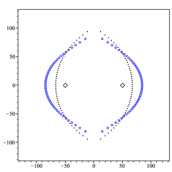
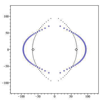
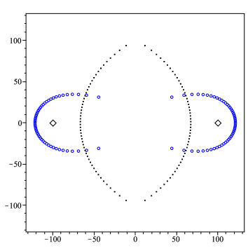
Figure 6: Zeros and poles (circles in the left and right-half planes respectively) of 2-point Padé approximants of degree (51,50) with two real interpolation points (diamonds) of multiplicity 51 located at $\{-50,50\}$, $\{-65,65\}$, $\{-85,85\}$, $\{-100,100\}$. For comparison, the zeros and poles of the Padé approximant of degree 50 are shown with dots.

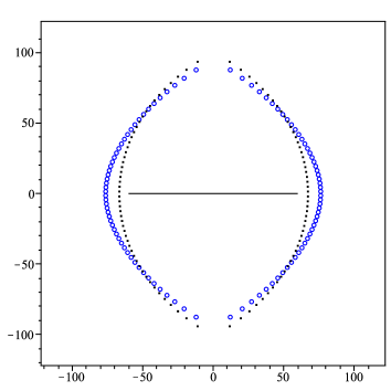
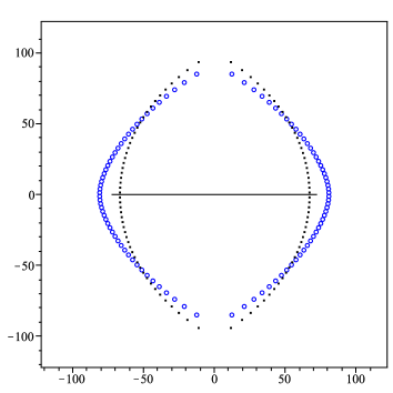
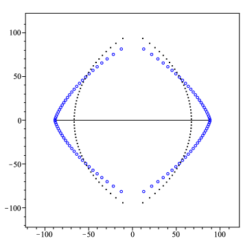
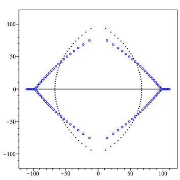
Figure 7: Zeros and poles (circles in the left and right-half planes respectively) of rational interpolants of degree 50 corresponding to 101 interpolation points regularly distributed on the real segments $60I,72.5I,87.5I,110I$, $I=[-1,1]$. For comparison, the zeros and poles of the Padé approximant of degree 50 are shown with dots.

In this section, we are interested in the location of zeros and poles of rational interpolants associated to interpolation points whose moduli are comparable to the degree of the interpolant. For the particular case of shifted Padé approximants $p_{n}^{(\xi_{n})}/q_{n}^{(\xi_{n})}$ interpolating the exponential function at $\xi_{n}$, we have the simple relation

$$\frac{p_{n}^{(\xi_{n})}(z)}{q_{n}^{(\xi_{n})}(z)}=e^{\xi_{n}}\frac{p_{n}^{(0)}(z-\xi_{n})}{q_{n}^{(0)}(z-\xi_{n})},$$

where $p_{n}^{(0)}(z)/q_{n}^{(0)}(z)$ denotes the usual Padé approximant interpolating $e^{z}$ at 0. Hence, we know at once that the distributions of poles and zeros follow exactly the shift of the interpolation point $\xi_{n}$ . In particular, the limit distributions of the scaled (by $2n$) zeros and poles are modified if and only if $\xi_{n}/n$ does not tend to 0, as $n$ tends to infinity.

In Figure 6, we consider the case of 2-point Padé approximants with two real symmetric interpolation points of equal multiplicities. As the points approach the zeros and poles of the usual Padé approximant (or equivalently, in the scaled situation, the critical curves $\gamma_{1}$ and $\gamma_{2}$), we can see how the distributions of zeros and poles are modified. Clearly, a repulsion takes place between the interpolation points and the zeros and poles of the approximants. In Figure 7, we consider the case of interpolation points regularly distributed on a real segment. As the segment approaches the zeros and poles of the usual Padé approximant, we can again observe how the distributions of zeros and poles are modified. Finally, in Figure 8, the case of interpolation points regularly distributed on a circle is depicted. The zeros and poles of the interpolants seem to be pushed away as the circle intersects the limit distributions corresponding to the usual Padé approximant.

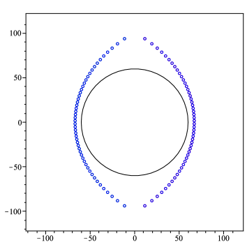
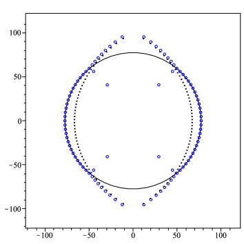
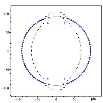
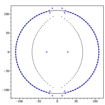
Figure 8: Zeros and poles (circles in the left and right-half planes respectively) of rational interpolants of degree 50 corresponding to 101 interpolation points regularly distributed on the circles of radius 60, 77.5, 92.5, and 110. For comparison, the zeros and poles of the Padé approximant of degree 50 are shown with dots.

From a theoretical point of view, polynomials whose roots are the above zeros and poles still satisfy the orthogonality relations (2.4). We note that, in the corresponding potential (2.2), the sum of log terms becomes preponderant as the interpolation points grow faster with $n$. This should account for the modification in the zeros and poles distributions of the rational interpolants, that we observe in our experiments. In any case, it would be interesting to study in more detail the interaction between the interpolation points and the zeros and poles of the approximants.

Tom Claeys, tom.claeys@uclouvain.be
Université Catholique de Louvain
Chemin du cyclotron 2
B-1348 Louvain-La-Neuve, BELGIUM

Franck Wielonsky, wielonsky@cmi.univ-mrs.fr
Laboratoire LATP - UMR CNRS 6632 Université de Provence
CMI 39 Rue Joliot Curie
F-13453 Marseille Cedex 20, FRANCE

References

- [1] M. Abramowitz and I.A. Stegun, Handbook of Mathematical Functions, Dover Publications, New York, 1968.
- [2] L. Baratchart, E.B. Saff, F. Wielonsky, Rational interpolation of the exponential function, Canad. J. of Math. 47, (1995), 1121-1147.
- [3] P.B. Borwein, Rational interpolation to , J. Approx. Theory 35 (1982), 142-147.
- [4] P.B. Borwein, Rational interpolation to , II, SIAM J. Math. Anal. 16 (1985), 656-662.
- [5] P. Deift, “ Orthogonal Polynomials and Random Matrices: A Riemann-Hilbert Approach”, Courant Lecture Notes 3, New York University 1999.
- [6] P. Deift, T. Kriecherbauer, K.T-R McLaughlin, S. Venakides, and X. Zhou, Uniform asymptotics for polynomials orthogonal with respect to varying exponential weights and applications to universality questions in random matrix theory, Comm. Pure Appl. Math. 52 (1999), 1335-1425.
- [7] P. Deift, T. Kriecherbauer, K.T-R McLaughlin, S. Venakides, and X. Zhou, Strong asymptotics of orthogonal polynomials with respect to exponential weights, Comm. Pure Appl. Math. 52 (1999), 1491-1552.
- [8] P. Deift and X. Zhou, A steepest descent method for oscillatory Riemann-Hilbert problems. Asymptotics for the MKdV equation, Ann. Math. 137 (1993), no. 2, 295-368.
- [9] K.A. Driver, N.M. Temme, Zero and pole distribution of diagonal Padé approximants to the exponential function, Quaest. Math. 22 (1999), 7–17.
- [10] A.A. Gonchar, E.A. Rakhmanov, Equilibrium distributions and degree of rational approximation of analytic functions, Math. USSR Sbornik 62 (1989), 305-348.
- [11] A. Kuijlaars, H. Stahl, W. Van Assche, F. Wielonsky, Type II Hermite–Padé approximation to the exponential function, J. Comp. and Appl. Math., 207 (2007), 227–244.
- [12] A.B.J. Kuijlaars, W. Van Assche, and F. Wielonsky, Quadratic Hermite-Padé approximation to the exponential function: a Riemann–Hilbert approach, Constr. Approx. 21 (2005), 351–412.
- [13] E.B. Saff and V. Totik, “ Logarithmic Potentials with External Fields”, Springer-Verlag, New-York (1997).
- [14] E.B. Saff and R.S. Varga, On the zeros and poles of Padé approximants to , Numer. Math. 25 (1975), 1–14.
- [15] E.B. Saff and R.S. Varga, On the zeros and poles of Padé approximants to . II., Padé and rational approximations: theory and applications (E.B. Saff, R.S. Varga, eds.), pp. 195–213, Academic Press, New York, 1977.
- [16] E.B. Saff and R.S. Varga, On the zeros and poles of Padé approximants to . III., Numer. Math. 30 (1978), 241–266.
- [17] H. Stahl, Quadratic Hermite-Padé polynomials associated with the exponential function, J. Approx. Theory 125 (2003), 238-294.
- [18] H. Stahl, From Taylor to quadratic Hermite-Padé polynomials, Electron. Trans. Numer. Anal. 25 (2006), 480-510.
- [19] R.S. Varga and A.J. Carpenter, Asymptotics for the zeros and poles of normalized Padé approximants to , Numer. Math. 68 (1994), 169–185.
- [20] F. Wielonsky, On rational approximation to the exponential function with complex conjugate interpolation points, J. Approx. Theory 111 (2001), 344-368.
- [21] F. Wielonsky, Riemann-Hilbert analysis and uniform convergence of rational interpolants to the exponential function, J. Approx. Theory 131 (2004), 100–148.
- [22] F. Wielonsky, A note on the convergence of shifted Padé approximants to the exponential function, Manuscript (2011).