Conservative Initial Mapping For Multidimensional Simulations of Stellar Explosions

Abstract

Mapping one-dimensional stellar profiles onto multidimensional grids as initial conditions for hydrodynamics calculations can lead to numerical artifacts, one of the most severe of which is the violation of conservation laws for physical quantities such as energy and mass. Here we introduce a numerical scheme for mapping one-dimensional spherically-symmetric data onto multidimensional meshes so that these physical quantities are conserved. We validate our scheme by porting a realistic 1D Lagrangian stellar profile to the new multidimensional Eulerian hydro code CASTRO. Our results show that all important features in the profiles are reproduced on the new grid and that conservation laws are enforced at all resolutions after mapping.

1 Introduction

Multidimensional simulations shed light on how fluid instabilities arising in supernova explosions mix ejecta [1, 2, 3, 4]. Unfortunately, computing the full self-consistent three-dimensional (3D) stellar evolution initial models for the explosion setup is still beyond the realm of contemporary computational power. One alternative is to first evolve the main sequence star in a 1D stellar evolution code in which the equations of momentum, energy and mass are solved on a spherically symmetric Lagrangian grid, such as KEPLER [5] or MESA [6]. Once the star reaches the pre-supernova phase, its 1D profiles can then be mapped into multidimensional hydro codes such as CASTRO [7, 8] or FLASH [9] and continue to be evolved until the star explodes.

Differences between codes in dimensionality and coordinate mesh can lead to numerical issues such as violation of conservation of mass and energy when profiles are mapped from one code to another. A first, simple approach could be to initialize multidimensional grids by linear interpolation from corresponding mesh points on the 1D profiles. However, linear interpolation becomes invalid when the new grid fails to resolve critical features in the original profile such as the inner core of a star. This is especially true when porting profiles from 1D Lagrangian codes, which can easily resolve very small spatial features in mass coordinate, to a fixed or adaptive Eulerian grid. Besides conservation laws, some physical processes such as nuclear burning are very sensitive to temperature, so slight errors in mapping can lead to very different outcomes for the simulation. Only a few studies have examined mapping 1D profiles to 2D or 3D meshes [10], and none address the conservation of physical quantities by such procedures.

We investigate these issues and introduce a new scheme for mapping 1D data sets to multidimensional grids. We first describe our mapping algorithm in § 2 and then present results of porting a massive star model from KEPLER to CASTRO in § 3. Finally, we conclude in § 4.

2 Method

Since the star is very nearly in hydrostatic equilibrium but we also map explosions where we want to conserve the total energy , care must be taken in mapping its profile from the non-uniform Lagrangian grid in mass coordinate to the new Eulerian spatial grid. Our method preserves conservation of quantities such as mass and energy that are analytically conserved in the evolution equations on the new mesh. Although this does not guarantee that a hydrostatic star will be fully hydrostatic on the new grid because our construction does not, it is a physically motivated constraint and sufficient for our simulations. The algorithm we describe below is specific to our stellar models but can be easily generalized to other mappings of 1D data to higher dimensions.

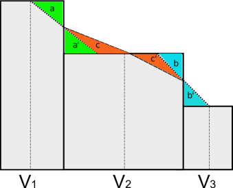
Figure 1: Constructing a conservative profile. The rectangular bins illustrate the original 1D profile. The areas of different colors represent conserved quantities such as mass and internal energy. Note that uniform zones in mass lead to nonuniform bins in volume coordinate, as shown above.

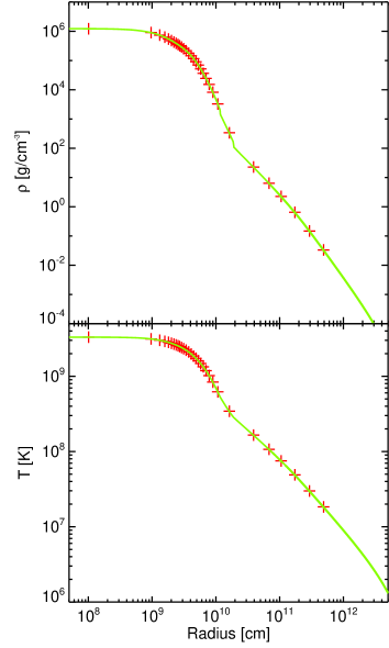
Figure 2: KEPLER densities and temperatures (red crosses) and our piecewise linear fits (green lines). Since we map internal energy (a conserved quantity) rather than temperature, we calculate $T$ from the equation of state using density, element abundance, and internal energy.

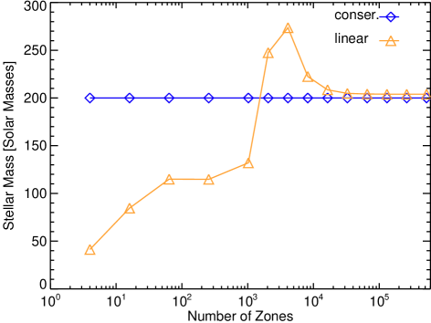
Figure 3: Total mass of the star on the new 1D CASTRO grid vs. number of zones. Conservative mapping (blue) preserves the mass of the star at all resolutions, while linear interpolation (orange) converges to 200 $\mathrm{M}_{\odot}$ at a resolution of $\sim$ a few $\times 10^{4}$, when the grid begins to resolve the core of the star ($\sim 10^{9}$ cm). Even using a very high resolution, the linear interpolation still fails to resolve the density gradient between the inner core and the out envelope (see Figure 2 $10^{9}\sim 10^{11}$ cm). So the curve of linear interpolation is saturated at zone number $\sim 10^{5}$, its results are still off by a few $\%$.

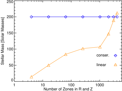
Figure 4: Total mass of the star on the new 2D CASTRO grid vs. number of zones in both $r$ and $z$. Conservative mapping (blue) recovers the mass of the star at all resolutions and linear interpolation (orange) approaches 200 $\mathrm{M}_{\odot}$ at a resolution of $\sim$ $2048^{2}$.

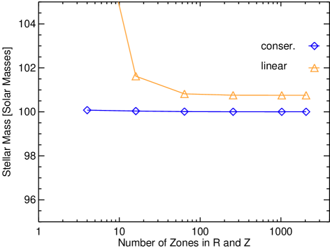
Figure 5: Total mass of the He core on the 2D CASTRO grid vs. number of zones in both $r$ and $z$. Conservative mapping (blue) preserves the original mass of the core at all resolutions while linear interpolation (orange) begins to converge to 100 $\mathrm{M}_{\odot}$ at a resolution of $64^{2}$ but is still off by $\sim 1\%$ even as the resolution approaches $\sim 2048^{2}$ .

First, we construct a continuous (C⁰) function that conserves the physical quantity when it is mapped onto the new grid. An ideal choice for interpolation is the volume coordinate $V$, the volume enclosed by a given radius from the center of the star. Then, integrating a density $\rho_{X}$ (which can represent mass or internal energy density) with respect to the volume coordinate yields a conserved quantity $X$

$$X=\int_{V_{1}}^{V_{2}}\rho_{X}\,\mathrm{d}V,$$ (1)

such as the total mass or internal total energy lying in the shell between $V_{1}$ and $V_{2}$.

Next, we define a piecewise linear function in volume $V$ that represents the conserved quantity $\rho_{X}$, preserves its monotonicity (no new artificial extrema), and is bounded by the extrema of the original data. The segments are constructed in two stages. First, we extend a line across the interface between adjacent zones that either ends or begins at the center of the smaller of the two zones, as shown in Figure 1 (note that uniform zones in mass coordinate do not result in uniform zones in $V$). The slope of the segment is chosen so that the area trimmed from one zone by the segment ($a$ and $b$) is equal to the area added under the segment in the neighboring bin ($a^{\prime}=a$ and $b^{\prime}=b$).

If the two segments bounding $a$ and $a^{\prime}$ and $b$ and $b^{\prime}$ are joined together by a third in the center zone in Figure 1, two “kinks”, or changes in slope, can arise in the interpolated quantity there; plus, the slope of the flat central segment is usually a poor approximation to the average gradient in that interval. We therefore construct two new segments that span the entire central zone and connect with the two original segments where they cross its interfaces, as shown in Figure 1. The new segments join each other at the position in the central bin where the areas $c$ and $c^{\prime}$ enclosed by the two segments are equal (note that they in general have different slopes). After repeating this procedure everywhere on the grid, each bin will be spanned by two linear segments that represent the interpolated quantity $\rho_{X}$ at any $V$ within the bin and have no more than one kink in $\rho_{X}$ across the zone. Our scheme introduces some smearing (or smoothing) of the data, but it is limited to less than or equal to the width of one zone on the original grid.

The result of our interpolation scheme is a piecewise linear reconstruction in $V$ of the original profile in mass coordinate, for which the quantity $\rho_{X}$ can be determined at any $V$, not just the radii associated with the Lagrangian grid. We show this profile as a function of the radius associated with the volume coordinate $V$ for a zero-metallicity 200 $\mathrm{M}_{\odot}$ star with $r$ $\sim$ $2\times 10^{13}$ cm from KEPLER [11, 12] in Figure 2.

We populate the new multidimensional grid with conserved quantities from the reconstructed stellar profiles as follows. First, the distance of the selected mesh point from the center of the new coordinate grid is calculated. We then use this radius to obtain its $V$ to reference the corresponding density in the piecewise linear profile of the star. The density assigned to the zone is then determined from adaptive iterative subsampling. This is done by first computing the total mass of the zone by multiplying its volume by the interpolated density. We then divide the zone into equal subvolumes whose sides are half the length of the original zone. New $V$ are computed for the radii to the center of each of these subvolumes and their densities are again read in from the reconstructed profile. The mass of each subvolume is then calculated by multiplying its interpolated density by its volume element. These masses are then summed and compared to the mass previously calculated for the entire cell. If the relative error between the two masses is larger than some predetermined tolerance, each subvolume is again divided as before, masses are computed for all the constituents comprising the original zone, and they are then summed and compared to the zone mass from the previous iteration. This process continues recursively until the relative error in mass between the two most recent consecutive iterations falls within an acceptable value, typically 10^-4. The density we assign to the zone is just this converged mass divided by the volume of the entire cell. This method is used to map internal energy density and the partial densities of the chemical species to every zone on the new grid. The total density is then obtained from the sum of the partial densities; pressure and temperature in turn are determined from the equation of state. This method is easily applied to hierarchy geometry of the target grid.

3 Results

We port a 1D stellar model from KEPLER into CASTRO to verify that our mapping is conservative. As an example here, we use the zero-metalicity pre-supernova 200 $\mathrm{M}_{\odot}$ star whose profiles are shown in Figure 2. KEPLER is a Lagrangian code that evolves stars in mass coordinate so its mesh is nonuniform in space, and CASTRO has an Eulerian grid with uniform spatial zones.

We compare our piecewise linear fits to the KEPLER data in Figure 2, which shows that they reproduce the original stellar profile. Because our fits smoothly interpolate the block histogram structure of the KEPLER bins (especially at larger radii), they reduce the number of unphysical sound waves that would have been introduced in CASTRO by the discontinuous interfaces between these bins in the original data. The density profile is key to the hydrodynamic and gravitational evolution of the explosion, and the temperature profile is crucial to the nuclear burning that powers the explosion.

We first map the profile onto a 1D grid in CASTRO and plot the mass of the star as a function of grid resolution in Figure 3. The mass is independent of resolution for our conservative mapping because we subsample the quantity in each cell prior to initializing it, as described above. In contrast, the total mass from linear interpolation is very sensitive to the number of grid points but does eventually converge when the number of zones is sufficient to resolve the core of the star, in which most of its mass resides.

We next map the KEPLER profile onto a 2D cylindrical grid ($r,z$) and a 3D cartesian grid ($x,y,z$) in CASTRO. The only difference between mapping to 1D, 2D, and 3D is the form of the volume elements used to subsample each cell, which are $4\pi r^{2}dr$, $2\pi rdrdz$, $dxdydz$, respectively. We show the mass of the star as a function of resolution in Figure 4. Conservative mapping again preserves its mass at all grid resolutions. In 2D, more zones are required for linear interpolation to converge to the mass of the star. To further validate our conservative scheme, we map just the helium core of star ($\sim$ 100 ${\mathrm{M}_{\odot}}$ with $r\sim$ 10¹⁰ cm) onto the 2D grid. The helium core is crucial to modeling thermonuclear supernovae because it is where explosive burning begins. We show its mass as a function of resolution in Figure 5. We again recover all the mass of the core at all resolutions while linear interpolation overestimates the mass by at least $\sim$ 1 $\%$, even with large numbers of zones.

Conservative mapping is effective in 3D but requires much more computational time to subsample each cell to convergence. Furthermore, an impractical number of zones is needed for linear interpolation to reproduce the original mass of the star, so we defer its comparison to our scheme in 3D to a later study. We note that our method also works with adaptive mesh refinement (AMR) grids because both $V$ and the interpolated quantities can be determined and subsampling can be performed on every grid in the hierarchy.

4 Conclusion

Multidimensional stellar evolution and supernova simulations are numerically challenging because multiple physical processes (hydrodynamics, gravity, burning) occur on many scales in space and time. For computational efficiency, 1D stellar models are often used as initial conditions in 2D and 3D calculations. Mapping 1D profiles onto multidimensional grids can introduce serious numerical artifacts, one of the most severe of which is the violation of conservation of physical quantities. We have developed a new mapping algorithm that guarantees that conserved quantities are preserved at any resolution and reproduces the most important features in the original profiles. Our method is practical for 1D and 2D calculations, and we are now developing integral methods (an explicit integral approach instead of using volume subsampling) that are numerically tractable in 3D.

References

References

- [1] Herant M and Woosley S E 1994 ApJ 425 814–828
- [2] Joggerst C C, Woosley S E and Heger A 2009 ApJ 693 1780–1802 (Preprint 0810.5142)
- [3] Joggerst C C, Almgren A, Bell J, Heger A, Whalen D and Woosley S E 2010 ApJ 709 11–26 (Preprint 0907.3885)
- [4] Joggerst C C and Whalen D J 2011 ApJL 728 129 (Preprint 1010.4360)
- [5] Weaver T A, Zimmerman G B and Woosley S E 1978 ApJ 225 1021–1029
- [6] Paxton B, Bildsten L, Dotter A, Herwig F, Lesaffre P and Timmes F 2011 ApJS 192 3 (Preprint 1009.1622)
- [7] Zhang W, Howell L, Almgren A, Burrows A and Bell J 2011 ApJS 196 20 (Preprint 1105.2466)
- [8] Almgren A S, Beckner V E, Bell J B, Day M S, Howell L H, Joggerst C C, Lijewski M J, Nonaka A, Singer M and Zingale M 2010 ApJ 715 1221–1238 (Preprint 1005.0114)
- [9] Fryxell B, Olson K, Ricker P, Timmes F X, Zingale M, Lamb D Q, MacNeice P, Rosner R, Truran J W and Tufo H 2000 ApJS 131 273–334
- [10] Zingale M, Dursi L J, ZuHone J, Calder A C, Fryxell B, Plewa T, Truran J W, Caceres A, Olson K, Ricker P M, Riley K, Rosner R, Siegel A, Timmes F X and Vladimirova N 2002 ApJS 143 539–565 (Preprint arXiv:astro-ph/0208031)
- [11] Heger A and Woosley S E 2002 ApJ 567 532–543 (Preprint arXiv:astro-ph/0107037)
- [12] Heger A and Woosley S E 2010 ApJ 724 341–373 (Preprint 0803.3161)