Spectral properties of one-dimensional spiral spin density wave states

Abstract

We provide a full characterization of the spectral properties of spiral spin density wave (SSDW) states which emerge in one-dimensional electron systems coupled to localized magnetic moments or quantum wires with spin-orbit interactions. We derive analytic results for the spectral function, local density of states and optical conductivity in the low-energy limit by using field theory techniques. We identify various collective modes and show that the spectrum strongly depends on the interaction strength between the electrons. The results provide characteristic signatures for an experimental detection of SSDW states.

It is by now well established that interactions have drastic effects on one-dimensional systems.Giamarchi04 For example, the spectral properties of Luttinger liquids, which one may regards as the standard model of one-dimensional electrons, show spin-charge separation as well as non-trivial power laws which depend on the interaction strength.LL The system decomposes into two gapless sectors describing collective charge and spin excitations which possess linear dispersion relations with velocities $v_{\text{c}}$ and $v_{\text{s}}$, respectively. More general situations can be described by adding appropriate terms to the Luttinger liquid Hamiltonian. For example, spin-orbit interactions (SOI) lead to a mixing of charge and spin degrees of freedom, which strongly affects the spectral function but leaves the system gapless.Schulz-09

A more profound change in the low-energy properties happens when the system develops a gap. The prototype scenarioGiamarchi04 for this situation is the Mott transition at which a gap in the charge sector opens provided the system is at commensurate filling. The spectral function of the resulting Mott insulator (MI)MI still shows spin-charge separation but the charge excitations possess a mass $\Delta$. A similar situation is encountered in systems with SOI and an additional magnetic field, where a spin gap opens while the charge sector remains gapless.Sun-07 On the other hand, if the SOI are spatially modulated with a wave length commensurate with the Fermi wave length, the system develops gaps in both sectors.Japaridze-09 In all three situations the system separates into charge and spin sectors, i.e., there is no non-trivial mixing of gapless and gapped degrees of freedom.

As it was shown by Braunecker et al.,Braunecker-09 this is no longer the case if one considers the interplay of one-dimensional electronic degrees of freedom and localized magnetic moments such as nuclear spins. In such systems feedback effects between the conduction electrons and nuclear magnetic moments can, at sufficiently low temperatures, stabilize the coexistence of electron density order and helical magnetic order. Specifically they showed that the electronic subsystem develops a gap in a superposition of charge and spin degrees of freedom accompanied by a spiral spin density wave (SSDW)SLL following the helical magnetic order. As the original electrons possess a highly non-trivial decomposition into the gapped and gapless sectors one expects the system to possess rather unusual spectral properties. We note that similar situations are encountered in Luttinger liquids coupled to extended ferromagnetic domain wallsPereiraMiranda04 as well as in quantum wires with SOI in a magnetic field along the wire provided the band shift induced by the SOI is commensurate with the Fermi momentum.Braunecker-10

In this Rapid Communication we provide a detailed analysis of the spectral properties of such SSDW states. We show that the spectral function is strongly asymmetric in the spin components and identify various dispersing collective modes. The calculated local density of states (LDOS) exhibits typical features of both the Luttinger liquid and the MI. In particular we are able to derive exact results for the appearing power-law exponents. Finally we show that the optical conductivity possesses characteristic singularities intimately related to the interactions between the electrons. Taken together our results provide a set of specific signatures necessary for the experimental identification of SSDW states.

Model. Experimental systems in which such states may exist require the interaction between electrons and nuclear spins in one dimension as it is, for example, the case in ¹³C single-wall carbon nanotubesCNT or GaAs quantum wires.GaAs Braunecker et al.Braunecker-09 showed that in these systems the conduction electrons mediate an RKKY interaction between the nuclear spins. The feedback of the resulting helical magnetic order causes the formation of a SSDW state and generates a gap in the electronic subsystem, which can be described by the effective low-energy Hamiltonian (which is also relevantBraunecker-10 to quantum wires with SOI showing a spin-selective Peierls transition)

$$H = H_{+}+H_{-},$$ (1)

$$H_{+} = \frac{v_{+}}{16\pi}\int\text{d}x\Bigl{[}\bigr{(}\partial_{x}\Phi_{+}\bigr{)}^{2}+\bigr{(}\partial_{x}\Theta_{+}\bigr{)}^{2}\Bigr{]}$$ (2)

$$+\frac{B}{2\pi}\int\text{d}x\,\cos\bigl{(}\sqrt{K/4}\,\Phi_{+}\bigr{)},$$

$$H_{-} = \frac{v_{-}}{16\pi}\int\text{d}x\Bigl{[}\bigr{(}\partial_{x}\Phi_{-}\bigr{)}^{2}+\bigr{(}\partial_{x}\Theta_{-}\bigr{)}^{2}\Bigr{]}.$$ (3)

Here $\Phi_{\pm}$ are canonical Bose fields and $\Theta_{\pm}$ are their dual fields. The velocities $v_{\pm}$ and the Luttinger parameter $K$ are related to the original parameters in the charge and spin sectors via

$$v_{+}=\frac{1}{K}\left[v_{\mathrm{c}}K_{\mathrm{c}}+\frac{v_{\mathrm{s}}}{K_{\mathrm{s}}}\right],\quad v_{-}=\frac{1}{K}\left[\frac{v_{\mathrm{c}}}{K_{\mathrm{s}}}+v_{\mathrm{s}}K_{\mathrm{c}}\right],$$ (4)

and $K=K_{\text{c}}+1/K_{\text{s}}$. For $K<4$ the cosine term in (2) is relevant and generates a gap $\Delta$, which is a functionZamolodchikov95 of the bare Overhauser field $B$ and $K$. We will view it here as a phenomenological parameter replacing $B$ such that we are left with the four free parameters $K_{\text{c,s}}$, $v_{\text{c}}/v_{\text{s}}$, and $\Delta$. For repulsive electron-electron interactions one has $0<K_{\text{c}}<1$. Furthermore, in the derivation of (1) it was assumed thatBraunecker-09 $K_{\text{s}}\geq 1$, where $K_{\text{s}}=1$ corresponds to the spin rotational invariant situation.

The bosonic fields appearing in (1) are related to the slowly varying right- and left-moving Fermi fields defined via

$$\Psi_{\sigma}(x)=e^{\text{i}k_{\text{F}}x}\psi_{\text{R}\sigma}(x)+e^{-\text{i}k_{\text{F}}x}\psi_{\text{L}\sigma}(x),$$ (5)

by the relationsBraunecker-09 ($l=\text{R/L}\equiv\pm$, $\sigma=\uparrow,\downarrow\equiv\pm$)

$$\psi_{\pm\pm} = \frac{\eta_{\pm\pm}}{\sqrt{2\pi}}\,\exp\bigl{(}\mp\text{i}a\Phi_{+}\bigr{)}\,\exp\bigl{(}\pm\text{i}b\Phi_{-}-\text{i}c\Theta_{-}\bigr{)},$$ (6)

$$\psi_{\pm\mp} = \frac{\eta_{\pm\mp}}{\sqrt{2\pi}}\,\exp\bigl{(}\tfrac{\text{i}}{2\sqrt{K}}\Theta_{+}\mp\text{i}\tfrac{\sqrt{K}}{4}\Phi_{+}\bigr{)}\,\exp\bigl{(}\text{i}d\Theta_{-}\bigr{)},\quad$$ (7)

where the Klein factors $\eta_{l\sigma}$ satisfy the anticommutation relations $\{\eta_{l\sigma},\eta_{l^{\prime}\sigma^{\prime}}\}=2\delta_{ll}\delta_{\sigma\sigma^{\prime}}$ and the constants are defined by $a=(K_{\text{c}}K_{\text{s}}-1)/(4K_{\text{s}}\sqrt{K})$, $b=\sqrt{K_{\text{c}}/(KK_{\text{s}})}/2$, and $c,d=(K_{\text{c}}K_{\text{s}}\pm 1)/(4\sqrt{KK_{\text{c}}K_{\text{s}}})$.

The excitations in the sine-Gordon model (2) are solitons and antisolitons with mass $\Delta$, and, if $K<4/(N+1)$, breather (soliton-antisoliton) bound states $B_{n}$, $n=1,\ldots,N$, with masses $\Delta_{n}=2\Delta\sin(n\pi K/(8-2K))$. We note that there exists at least one breather for repulsive interactions. The solitons and antisolitons possess a relativistic dispersion relation $E^{2}=\Delta^{2}+v_{+}^{2}P^{2}$; the dispersion relation for the $n$th breather is obtained by replacing $\Delta$ by $\Delta_{n}$. The sector (3) describes gapless collective excitations propagating with velocity $v_{-}$.

Green’s function. The spin-resolved spectral function and LDOS discussed below follow from the spin-diagonal Green’s function in Euclidean space, which is defined by

$$G_{\sigma}(\tau,x)=\sum_{ll^{\prime}}e^{\text{i}lk_{\text{F}}x}\,G_{\sigma}^{ll^{\prime}}(\tau,x),$$ (8)

where $G^{ll^{\prime}}_{\sigma}(\tau,x)=-\langle\mathcal{T}_{\tau}\,\psi_{l\sigma}(\tau,x)\,\psi_{l^{\prime}\sigma}^{\dagger}(0,0)\rangle$, $\tau=\text{i}t$ denotes Euclidean time, and $\mathcal{T}_{\tau}$ is the $\tau$-ordering operator. Due to the decomposition of the Hamiltonian the Green’s function factorizes into a product of correlation functions in the gapped and gapless sectors. The correlation functions in the gapless sector can be straightforwardly calculated by using standard methods.Giamarchi04 The derivation in the gapped sector employs the integrability of the sine-Gordon model via a form-factor expansionSmirnov92book ; EsslerKonik05 with the results (${\tau>0}$)

$$\begin{split}&G^{\text{RR}}_{\uparrow}(\tau,x)=-\frac{1}{2\pi}\frac{1}{(v_{-}\tau-\text{i}x)^{2(b+c)^{2}}}\frac{1}{(v_{-}\tau+\text{i}x)^{2(b-c)^{2}}}\\ &\;\times G_{a}^{2}\left[1+\frac{\lambda^{2}\sin^{2}\tfrac{2\pi\sqrt{K}a}{4-K}}{\pi\sin^{2}\tfrac{\pi K}{4-K}}K_{0}\Bigl{(}\Delta_{1}\sqrt{\tau^{2}+x^{2}/v_{+}^{2}}\Bigr{)}+\ldots\right]\end{split}$$ (9)

and

$$\begin{split}&G^{\text{RR}}_{\downarrow}(\tau,x)=-\frac{1}{2\pi}\frac{1}{(v_{-}\tau-\text{i}x)^{2d^{2}}}\frac{1}{(v_{-}\tau+\text{i}x)^{2d^{2}}}\\ &\;\times\left[\frac{Z_{1}}{\pi}\left(\frac{v_{+}\tau+\text{i}x}{v_{+}\tau-\text{i}x}\right)^{\tfrac{1}{4}}K_{1}\Bigl{(}\Delta\sqrt{\tau^{2}+x^{2}/v_{+}^{2}}\Bigr{)}+\ldots\right].\end{split}$$ (10)

Here $K_{0/1}$ denote modified Bessel functionsAS and the constants $G_{a}$, $\lambda$, and $Z_{1}$ (which depend on $K_{\text{c}}$ and $K_{\text{s}}$) were obtained in Refs. LukyanovZamolodchikov97, ; FF, . The subleading terms in (9) and (10) involve heavier breathers $B_{n}$, $n\geq 2$ (for $K<4/3$), or multi-particle states. Furthermore we have $G_{\sigma}^{\text{LL}}(\tau,x)=G_{\bar{\sigma}}^{\text{RR}}(\tau,-x)$, $G_{\sigma}^{ll}(-\tau,-x)=G_{\sigma}^{ll}(\tau,x)$, and $G_{\sigma}^{\text{RL}}=G_{\sigma}^{\text{LR}}=0$ with $\bar{\sigma}=\mp$ for $\sigma=\pm$.

Spectral function. The spectral function can be experimentally probed using angle-resolved photoemission measurements. We can obtain the spin-resolved spectral function $A_{\sigma}(\omega,p)=A^{>}_{\sigma}(\omega,p)+A^{<}_{\sigma}(\omega,p)$ directly from the Green’s function (8) via

$$A^{\gtrless}_{\sigma}(\omega,p)=\mp\int\frac{\text{d}t}{2\pi}\frac{\text{d}x}{2\pi}\,e^{\text{i}(\omega t-px)}\,G_{\sigma}(\tau\gtrless 0,x)\Bigl{|}_{\tau\to\text{i}t\pm\delta},$$ (11)

where $\delta$ is small but finite and mimics broadening by instrumental resolution and temperature in experiments. The form-factor expansions (9) and (10) result in a similar expansion for the spectral function, where each term can be expressed as an integral over a hypergeometric function depending on the parameters $b,c$, and $d$. We note that the multi-particle corrections to (9) and (10) yield negligibleFFexpansion contributions at low energies and vanish for $|\omega|<2\Delta$. The spectral function satisfies $A_{\sigma}(-\omega,k_{\text{F}}-q)=A_{\sigma}(\omega,k_{\text{F}}+q)$ and $A_{\sigma}(\omega,-k_{\text{F}}-q)=A_{\bar{\sigma}}(\omega,k_{\text{F}}+q)$.

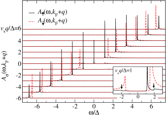
Figure 1: (Color online) Spectral function $A_{\sigma}(\omega,k_{\text{F}}+q)$ for $K_{\text{c}}=0.5$, $K_{\text{s}}=1$, $v_{\text{c}}=1.2\,v_{\text{s}}$, $\sigma=\uparrow$ (solid black lines), and $\sigma=\downarrow$ (dashed red lines). The curves are constant $q$-scans which have been offset along the $y$-axis with respect to one another. We stress that the up-spin component possesses spectral weight within the gap $\Delta$ and that the dispersions cross at $v_{\text{s}}q_{0}/\Delta\approx\pm 2.6$. The arrows in the inset indicate the energies where processes involving $B_{1}$ set in.

The spectral function in the vicinity of $p=k_{\text{F}}$ is shown in Fig. 1. We observe a strong spin dependence. The up-spin component is dominated by a linearly dispersing feature following $\omega=v_{-}q$ which originates from the gapless excitations of (3). In addition the existence of breathers results in dispersing features at $\omega=\pm(\Delta_{n}^{2}+v_{+}^{2}q^{2})^{1/2}$ which are, however, very weak (see the arrows in the inset in Fig. 1). From our analytical results we can extract the power laws at the dispersing features, e.g., for fixed $q>0$ and $\delta\to 0^{+}$, we obtain

$$A_{\uparrow}(\omega,k_{\text{F}}\pm q)\propto(\omega-v_{-}q)^{2(b\mp c)^{2}-1},\;\omega\to v_{-}q^{+},$$ (12)

while at $q=0$ the exponent is $4(b^{2}+c^{2})-2$. The measurement of these power laws can be used to extract the interaction strength encoded in the Luttinger parameters $K_{\text{c}}$ and $K_{\text{s}}$. We note that the derivationBraunecker-09 of the effective low-energy model (1) relied on a linear single-particle dispersion, whereas in any realistic microscopic model some curvature will be present. Although this curvature is irrelevant in the renormalization-group sense, it has been showncurvature to affect the power laws in the spectral function. However, as was argued in Ref. Braunecker-09, for both single-wall carbon nanotubes and GaAs quantum wires the curvature-induced deviations from (1) are negligible. We further note that a potentially present momentum dependence of the two-particle interactionMeden99 was neglected in the derivationBraunecker-09 of (1).

The down-spin component of the spectral function is dominated for $q>0$ by a dispersing mode following $\omega=\omega_{q}\equiv(\Delta^{2}+v_{+}^{2}q^{2})^{1/2}$ for which we find

$$A_{\downarrow}(\omega,k_{\text{F}}+q)\propto(\omega-\omega_{q})^{4d^{2}-1},\;\omega\to\omega_{q}^{+}.$$ (13)

In addition, there is a very weak feature at $\omega=-\omega_{q}$. The dispersing modes for $q<0$ are obtained using the symmetry of the spectral function. These dispersing features originate from the massive soliton excitations of (2), in particular the spectral function vanishes for $|\omega|<\Delta$. For generic system parameters one has $v_{\text{c}}>v_{\text{s}}$ and $K_{\text{c}}K_{\text{s}}<1$, which results in a crossing of the dispersing up- and down-spin features at $q_{0}=\pm\Delta/(v_{-}^{2}-v_{+}^{2})^{1/2}$. In the non-interacting case, ${K_{\text{c}}=K_{\text{s}}=1,v_{\text{c}}=v_{\text{s}}\equiv v}$, the contributions from the breathers vanish and the remaining dispersing features become $\delta$-functions, e.g., ${A_{\uparrow}(\omega,k_{\text{F}}+q)}\propto\delta(\omega-vq)$.

The vanishing of $A_{\downarrow}(\omega,k_{\text{F}}+q)$ and $A_{\uparrow}(\omega,-k_{\text{F}}-q)$ for $|\omega|<\Delta$ shows that the system effectively acts as a spin filter at sufficiently low energies. As was pointed out in Ref. Braunecker-09, , the existence of a gap in one half of the conduction channels yields a reduction of the conductance by a factor of 2. We note, however, that an experimental detection in transport experiments may be hampered by the influence of the attached contacts.conductance

Finally let us compare our results to the one-dimensional MI, whose spectral functionMI does not depend on the spin, possesses a gap, and clearly displays propagating charge and spin excitations. Thus although the low-energy theories of the MI and the SSDW state are both given by a sum of a gapped and a gapless sector, their spectral functions differ significantly due to the non-trivial decomposition of the electronic degrees of freedom into elementary excitations in the latter. In particular, the dispersing features in the SSDW state do not permit a simple interpretation in terms of individually propagating charge and spin excitations, i.e., a direct observation of spin-charge separation in a SSDW state is not possible. Furthermore the operator $e^{\mp\text{i}a\Phi_{+}}$ appearing in (6) possesses a non-vanishing vacuum expectation valueLukyanovZamolodchikov97 and thus gives rise to spectral weight at energies $|\omega|<\Delta$.

LDOS. Scanning tunneling microscopy (STM) and spectroscopy experiments measure the tunneling current between the sample and the STM tip as a function of the position of the tip and the applied voltage. The tunneling current is directly related to the LDOS of the sample, which is thus accessible in STM experiments. The LDOS $\rho(\omega)$ is obtained from the spectral function by integrating over the momentum. The result is spin independent and plotted in Fig. 2. We note that the LDOS has recently been calculatedBraunecker-11 by using a self-consistent harmonic approximation for the gapped sector, i.e., by expanding the cosine in (2) up to quadratic order.

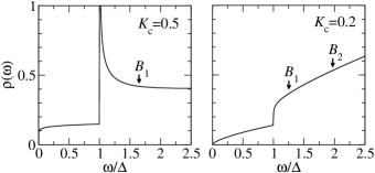
Figure 2: LDOS for $K_{\text{c}}=0.5$ (left panel) and $K_{\text{c}}=0.2$ (right panel), $K_{\text{s}}=1$, and $v_{\text{c}}=1.2\,v_{\text{s}}$. We observe a power-law behavior for $\omega\to 0$ [see Eq. (14)]. The singularity at $\omega=\Delta$ is only present for $K_{\text{c}}>\sqrt{5}-2$ [see Eq. (15)]. The arrows indicate the energies where single-breather processes set in.

The low-energy behavior of the LDOS can be determined from the first term in (9). We find for $|\omega|<\Delta$

$$\rho(\omega)\propto|\omega|^{\alpha},\;\alpha=4(b^{2}+c^{2})-1=\frac{\bigl{[}1+K_{\text{c}}(K_{\text{s}}-2)\bigr{]}^{2}}{4K_{\text{c}}(1+K_{\text{c}}K_{\text{s}})},$$ (14)

in agreement with the harmonic approximation.Braunecker-11 This again highlights the existence of spectral weight within the gap in contrast to the MI.MI In addition the LDOS possesses a pronounced feature at $\omega=\Delta$ at which the gapped sector (2) starts to contribute. For ${\omega\to\Delta^{+}}$ the leading term in (10) results in

$$\begin{split}&\rho(\omega)\propto(\omega-\Delta)^{\beta}+\ldots,\\ &\beta=4d^{2}-\frac{1}{2}=\frac{1+K_{\text{c}}^{2}K_{\text{s}}(K_{\text{s}}-2)-2K_{\text{c}}(1+K_{\text{s}})}{4K_{\text{c}}(1+K_{\text{c}}K_{\text{s}})},\end{split}$$ (15)

where the dots represent the regular background (14). We note that except for the non-interacting case, where $\beta=-1/2$, the exponent differs from the corresponding result of Ref. Braunecker-11, , as the harmonic approximation applied there does not correctly capture the Lorentz spin of solitons and antisolitons.

The most pronounced feature of the LDOS is found at $\omega=\Delta$, which is identical to the gap observed in ${A_{\downarrow}(\omega,k_{\text{F}}+q)}$. Furthermore, the exponents $\alpha$ and $\beta$ are fixed by the Luttinger parameters determined from the spectral function thus providing a consistency check between the measurements. Alternatively, if only the LDOS is accessible but the system is spin-rotational invariant ($K_{\text{s}}=1$), there is a fixed relation between $\alpha$ and $\beta$, e.g., $\beta$ vanishes for $K_{\text{c}}<\sqrt{5}-2$. In any case the breather contributions to the LDOS are negligible (see Fig. 2).

Due to the translational invariance of the system the LDOS shows no signatures of propagating quasiparticles. In order to identify such features in STM experiments it is thus neccessary to study the spatial Fourier transform of the LDOS in systems with boundaries or impurities.STM

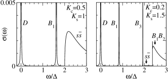
Figure 3: Conductivity for $v_{\text{c}}=1.2\,v_{\text{s}}$ and $K=1.5$ (left panel) as well as $K=0.87$ (right panel). We have convoluted the $\delta$-peaks by a Lorentzian. In both systems we observe the Drude peak ($D$) at $\omega=0$, the $\delta$-peak from the first breather $B_{1}$, and the soliton-antisoliton continuum ($s\bar{s}$). In the right-hand panel we further observe the $\delta$-peak from $B_{3}$ and the $B_{1}B_{2}$ continuum, which possesses a singularity at the lower threshold.

Conductivity. Finally let us discuss the optical conductivityGiamarchi04 $\sigma(\omega)$ which is obtained from the current-current correlation function. With the current densityGiamarchi04 ; Braunecker-09

$$j_{e}=\frac{e}{\pi}\partial_{t}\,\Phi_{\text{c}}=\frac{e}{\pi\sqrt{K}}\left[K_{\text{c}}\,\partial_{t}\,\Phi_{+}-\sqrt{\frac{K_{\text{c}}}{K_{\text{s}}}}\,\partial_{t}\,\Phi_{-}\right]$$ (16)

it follows that the conductivity is the sum of the conductivities in the gapped and gapless sectors, $\sigma(\omega)=\sigma_{+}(\omega)+\sigma_{-}(\omega)$. For the clean system we consider here the latter is given byGiamarchi04 a Drude peak $\propto\delta(\omega)$ while the former can be calculated analogously to a MI.Controzzi-01 Thus $\sigma_{+}(\omega)$ is given by a sum of $\delta$-functions originating in single-breather processes and, at higher frequencies, a many-particle continuum $\sigma_{+}^{\text{cont}}(\omega)$. As the current operator couples only to single-breather states with $n$ odd we find

$$\sigma_{+}(\omega)=\sum_{j=1}^{(N+1)/2}a_{j}\,\delta(\omega-\Delta_{2j-1})+\sigma_{+}^{\text{cont}}(\omega),$$ (17)

where the coefficients $a_{j}$ are fixed by the single-breather form factorsSmirnov92book ; EsslerKonik05 ; Controzzi-01 of the current operator.

For $4/3\leq K<2$ only the breather $B_{1}$ exists. As shown in the left-hand panel in Fig. 3 the conductivity is dominated by two $\delta$-peaks at low energies, while at $\omega>2\Delta$ the soliton-antisoliton ($s\bar{s}$) continuum shows up. In particular the optical gap is twice the gap observed in the spectral function or the LDOS. The leading corrections are given by the three-particle process $s\bar{s}B_{1}$ which sets in at $\omega=2\Delta+\Delta_{1}$. For $K<4/3$ the second breather starts to contribute in the two-breather continuum, but not as a single-particle peak as the current operator does not couple to $B_{2}$. As shown in the right-hand panel in Fig. 3, for $2/3\leq K<1$ a third $\delta$-peak originating in $B_{3}$ exists. The two-particle continuum is dominated by the two-breather process $B_{1}B_{2}$ while the soliton-antisoliton contribution is strongly suppressed as its spectral weight is transferred to the coherent $B_{1}$-peak. ($B_{1}$ is a $s\bar{s}$ bound state.) We stress that the $B_{1}B_{2}$-continuum possesses a singularity at the threshold $\omega\to(\Delta_{1}+\Delta_{2})^{+}$. The leading corrections are given by the three-particle processes $B_{1}B_{1}B_{1}$. We note that the condition $K<1$ requires the breaking of the spin rotation invariance, i.e., $K_{\text{s}}>1$. If $K$ is further decreased, the conductivity develops more features due to the existence of additional breathers.

In contrast to the spectral function and LDOS, the conductivity allows an efficient spectroscopy of the individual breather masses. In particular, the knowledge of the Luttinger parameters and thus $K$ gives a precise prediction for the number and masses of detectable individual breather states as well as features in the many-particle continuum. This provides a non-trivial consistency check between measurements of the optical conductivity and the spectral function or LDOS which has to be satisfied for a definite detection of a SSDW state.

Conclusions. In this Rapid Communication we have presented a complete characterization of the spectral properties of SSDW states, which appearBraunecker-09 in one-dimensional electron systems coupled to nuclear spins or quantum wires in a magnetic field and with SOI that are commensurate with the Fermi momentum.Braunecker-10 We calculated the spin-resolved spectral function, LDOS, and optical conductivity. We identified various collective modes and showed that the spectrum strongly depends on the interaction strength between the electrons. We discussed various consistency checks between the observables and thus between measurements of the spectral function, the LDOS, and the optical conductivity which should allow an unambiguous detection of a SSDW state in future experiments on ¹³C single-wall carbon nanotubes and GaAs quantum wires.

I would like to thank Bernd Braunecker, Volker Meden, Pascal Simon, and particularly Fabian Essler, for useful discussions. This work was supported by the German Research Foundation (DFG) through the Emmy-Noether Program.

References

- (1) T. Giamarchi, Quantum Physics in One Dimension (Oxford University Press, Oxford, UK, 2004).
- (2) V. Meden and K. Schönhammer, Phys. Rev. B 46, 15753 (1992); J. Voit, ibid. 47, 6740 (1993).
- (3) A. Schulz, A. De Martino, P. Ingenhoven, and R. Egger, Phys. Rev. B 79, 205432 (2009); A. Schulz, A. De Martino, and R. Egger, ibid. 82, 033407 (2010).
- (4) F. H. L. Essler and A. M. Tsvelik, Phys. Rev. B 65, 115117 (2002); Phys. Rev. Lett. 90, 126401 (2003).
- (5) J. Sun, S. Gangadharaiah, and O. A. Starykh, Phys. Rev. Lett. 98, 126408 (2007); S. Gangadharaiah, J. Sun, and O. A. Starykh, Phys. Rev. B 78, 054436 (2008).
- (6) G. I. Japaridze, H. Johannesson, and A. Ferraz, Phys. Rev. B 80, 041308(R) (2009); M. Malard, I. Grusha, G. I. Japaridze, and H. Johannesson, ibid. 84, 075466 (2011).
- (7) B. Braunecker, P. Simon, and D. Loss, Phys. Rev. Lett. 102, 116403 (2009); Phys. Rev. B 80, 165119 (2009).
- (8) This state was named ”spiral Luttinger liquid” in Ref. Braunecker-11, , but we stress that it possesses a spectral gap.
- (9) R. G. Pereira and E. Miranda, Phys. Rev. B 69, 140402 (2004); N. Sedlmayr, S. Eggert, and J. Sirker, ibid. 84, 024424 (2011).
- (10) B. Braunecker, G. I. Japaridze, J. Klinovaja, and D. Loss, Phys. Rev. B 82, 045127 (2010).
- (11) F. Simon, Ch. Kramberger, R. Pfeiffer, H. Kuzmany, V. Zólyomi, J. Kürti, P. M. Singer, and H. Alloul, Phys. Rev. Lett. 95, 017401 (2005); M. H. Rümmeli et al., J. Phys. Chem. C 111, 4094 (2007); H. O. H. Churchill, A. J. Bestwick, J. W. Harlow, F. Kuemmeth, D. Marcos, C. H. Stwertka, S. K. Watson, and C. M. Marcus, Nat. Phys. 5, 321 (2009).
- (12) C. H. L. Quay, T. L. Hughes, J. A. Sulpizio, L. N. Pfeiffer, K. W. Baldwin, K. W. West, D. Goldhaber-Gordon, and R. de Picciotto, Nat. Phys. 6, 336 (2010).
- (13) Al. B. Zamolodchikov, Int. J. Mod. Phys. A 10, 1125 (1995).
- (14) F. A. Smirnov, Form Factors in Completely Integrable Models of Quantum Field Theory (World Scientific, Singapore, 1992).
- (15) F. H. L. Essler and R. M. Konik, in From Fields to Strings: Circumnavigating Theoretical Physics (Ian Kogan Memorial Collection), edited by M. Shifman, A. Vainshtein, and J. Wheater (World Scientific, Singapore, 2005), Vol. I.
- (16) Handbook of Mathematical Functions, edited by M. Abramowitz and I. A. Stegun (Dover, New York, 1965).
- (17) S. Lukyanov and A. B. Zamolodchikov, Nucl. Phys. B 493, 571 (1997).
- (18) S. Lukyanov, Mod. Phys. Lett. A 12, 2543 (1997); S. Lukyanov and A. B. Zamolodchikov, Nucl. Phys. B 607, 437 (2001).
- (19) This is a well-known feature of form-factor expansions in massive field theories; see J. L. Cardy and G. Mussardo, Nucl. Phys. B 410, 451 (1993) and Ref. EsslerKonik05, .
- (20) M. Khodas, M. Pustilnik, A. Kamenev, and L. I. Glazman, Phys. Rev. B 76, 155402 (2007); R. G. Pereira, S. R. White, and I. Affleck, ibid. 79, 165113 (2009); A. Imambekov and L. I. Glazman, Science 323, 228 (2009); T. L. Schmidt, A. Imambekov, and L. I. Glazman, Phys. Rev. Lett. 104, 116403 (2010); F. H. L. Essler, Phys. Rev. B 81, 205120 (2010); R. G. Pereira and E. Sela, ibid. 82, 115324 (2010).
- (21) K. Schönhammer and V. Meden, Phys. Rev. B 47, 16205 (1993); V. Meden, ibid. 60, 4571 (1999).
- (22) I. Safi and H. J. Schulz, Phys. Rev. B 52, R17040 (1995); D. L. Maslov and M. Stone, ibid. 52, R5539 (1995); V. V. Ponomarenko, ibid. 52, R8666 (1995); K. Janzen, V. Meden, and K. Schönhammer, ibid. 74, 085301 (2006).
- (23) B. Braunecker, C. Bena, and P. Simon, Phys. Rev. B 85, 035136 (2012).
- (24) S. A. Kivelson, I. P. Bindloss, E. Fradkin, V. Oganesyan, J. M. Tranquada, A. Kapitulnik, and C. Howald, Rev. Mod. Phys. 75, 1201 (2003); D. Schuricht, F. H. L. Essler, A. Jaefari, and E. Fradkin, Phys. Rev. Lett. 101, 086403 (2008); Phys. Rev. B 83, 035111 (2011); I. Schneider and S. Eggert, Phys. Rev. Lett. 104, 036402 (2010); D. Schuricht, Phys. Rev. B 84, 045122 (2011).
- (25) D. Controzzi, F. H. L. Essler, and A. M. Tsvelik, Phys. Rev. Lett. 86, 680 (2001); F. H. L. Essler, F. Gebhard, and E. Jeckelmann, Phys. Rev. B 64, 125119 (2001).