Strategic Arrivals into Queueing Networks:
The Network Concert Queueing Game

Harsha Honnappa EE Department, University of Southern California, Los Angeles, CA 90089. Email: honnappa@usc.edu Rahul Jain EE & ISE Departments, University of Southern California, Los Angeles, CA 90089. Email: rahul.jain@usc.edu

Queueing networks are typically modelled assuming that the arrival process is exogenous, and unaffected by admission control, scheduling policies, etc. In many situations, however, users choose the time of their arrival strategically, taking delay and other metrics into account. In this paper, we develop a framework to study such strategic arrivals into queueing networks. We start by deriving a functional strong law of large numbers (FSLLN) approximation to the queueing network. In the fluid limit derived, we then study the population game wherein users strategically choose when to arrive, and upon arrival which of the $K$ queues to join. The queues start service at given times, which can potentially be different. We characterize the (strategic) arrival process at each of the queues, and the price of anarchy of the ensuing strategic arrival game. We then extend the analysis to multiple populations of users, each with a different cost metric. The equilibrium arrival profile and price of anarchy are derived. Finally, we present the methodology for exact equilibrium analysis. This, however, is tractable for only some simple cases such as two users arriving at a two node queueing network, which we then present. Strategic arrivals, Population games, Game theory, Queueing Networks.

1 Introduction

This paper is motivated by the following scenario: Users arriving at a concert, a game or at a store for Black Friday sales, where arriving before others is preferable, are faced with the dilemma of when to arrive. Should one arrive early before others and wait a while for service to start, or arrive late and wait less, and yet by which time the best seats or deals may already be gone? In such settings, when rational users make strategic decisions of timing, we cannot assume that the arrival process can be modelled by an exogenous renewal process such as a Poisson process. Furthermore, there may be multiple queues (which may start service at different times) and arriving users may have a choice of which queue to join.

Similarly, users downloading large files from a website often time their downloads to times of day when network congestion is expected to be lower (e.g., late at night.) Moreover, upon arrival (at the web-site), they may have to choose which server to download from. A natural question to ask is “Does an equilibrium arrival process exist”? If it does, is it efficient with respect to some metric? If not, can we bound the amount of inefficiency? We answer these questions by modeling this strategic arrival behavior as a game that we call the network concert queueing game. Such strategic analysis of queues was introduced in Juneja and Jain (2009), Jain et al. (2011) for a single server FIFO queue. In this paper, we extend that analysis to a network of queues.

In this paper, users choose their arrival time into a parallel queueing network wherein queues serve at different rates, and start service at different times. We assume servers are work-conserving with infinite buffers. Users can start to queue even before service starts, and do not renege or balk. We also consider that users may belong to multiple populations, each with different cost characteristics. The game is analyzed in the fluid approximation setting which offers significant analytical simplicity and tractability, while still capturing essential features of the problem. Each arriving user chooses a queue to join, and a time to arrive that minimizes a linear cost that is a weighted function of the waiting time and the service completion time. The service completion time of a user depends on the arrival time, and may be considered as a proxy for the latter metric.

We make two main contributions in this paper. Our first contribution is a fluid limit for the queueing model we introduce, wherein each user picks his time of arrival from a distribution. Thus, the inter-arrival times are not independent, and the arrival process need not be a renewal process in general. Functional strong law of large numbers approximation to the queue length process, the busy time and the virtual waiting time process at each queue is derived. Also of interest would be a diffusion limit (via the functional central limit theorem) for the various processes of interest in this non-standard queueing model. We have made some progress on this, and is on-going work.

Our second contribution is to take the fluid approximation derived above, and study the associated population game wherein each non-atomic user strategically picks a time of arrival, as well as a queue it would join. Existence of equilibria in such non-atomic games was established in Schmeidler (1973). We, however, argue its existence (and uniqueness) by construction. The equilibrium arrival profile turns out to be a uniform distribution over a time interval that we can determine. We also characterize the loss in social welfare due to strategically arriving users, and obtain an exact expression for the price of anarchy of the game.

While there has been a lot of work on studying pricing of queueing service (see Dube and Jain (2011), Hassin and Haviv (2003), Mendelson and Whang (1990), Naor (1969)), games of timing where the users choose an arrival time strategically are not so well-understood. The earliest such work is Glazer and Hassin (1983) in which a discrete population of users choose the time of their arrival strategically into an ?/M/1 queue, by minimizing the queueing delay. Problems with similar motivation have been considered in the transportation literature but they have focused on non-queueing theoretic fluid models with delay alone as a cost metric (Lindsey 2004). In contrast, the framework of Jain et al. (2011) is more general: Each user has a cost which is a function of the waiting time as well as the service completion time of the user (a proxy for the number of users who arrive before that user) - a significant motivation for users to arrive early in many scenarios. On the other hand, only a fluid approximation of the discrete population model is considered.

In Section 2, we first develop a path-wise description of the parameters describing the queueing network, and fluid limit approximations to these processes. Next, we analyze the strategic arrivals game in the fluid setting, for a single arriving population in Section 3, and derive the equilibrium arrival distribution and the price of anarchy of this game. In Section 4, we derive the equilibrium arrival profile for multiple populations with disparate arrival costs, and show that it is unique. We derive the price of anarchy of this game, show that in a special case, it is bounded above by 2. In Section 5, we illustrate the difficulty in doing exact equilibrium analysis for a finite population, and hence the importance of equilibrium analysis in the fluid limit. We conclude with a summary and discussion of further work in Section 6.

2 The Queueing Network: Model and Fluid Limit

Consider a queueing network with $K$ single server FIFO nodes in parallel. Each node starts service at some fixed time (which could be different from the other nodes), offers service with a finite service rate, and operates independently of the other nodes. Each users’ time of arrival is an i.i.d. random variable with a given distribution and known support such that users can arrive and queue up even before service starts. Note that inter-arrival times need not be independent. Service times are i.i.d., and independent of the arrival process. A user upon arrival joins one of the queues according to a given routing probability. Routing will be assumed independent of the arrival time process. We first develop the fluid limits for the queueing model introduced as the population size increases to $\infty$.

Let $(\Omega,\mathcal{F},P)$ be a probability space, and $\mathcal{D}^{K}:=\mathcal{D}^{K}[-T_{0},\infty)$ the space of $K$-dimensional “right-continuous with left limits”, or cadlag processes (see Durrett (2010), Billingsley (1968)). Suppose there are $n$ users arriving at the queueing network. Let $\xi_{i}:\Omega\rightarrow\{1,\cdots,K\}$ be a random variable such that user $i$ is routed to the $\xi_{i}(\omega)$th node in the network. Thus, $p_{0,k}=P(\xi_{i}=k)$.

Let $T_{i}:\Omega\rightarrow[-T_{0},T]$ be the arrival time of user $i$, and $F$ the arrival time distribution. Denote $\mathbf{A}^{n}(t):=(A^{n}_{1}(t),\cdots,A^{n}_{K}(t))\in\mathcal{D}^{K}$, where $A^{n}_{K}(t)$ counts the number of arrivals at queue $k$, i.e.,

$$A^{n}_{k}(t):=\sum_{i=1}^{n}\mathbf{1}_{\{T_{i}\leq t\}}\mathbf{1}_{\{\xi_{i}=k\}},\quad\forall t\in[-T_{0},T],$$ (1)

where $\mathbf{1}_{\{\cdot\}}$ denotes the indicator function. Let $A^{n}(t)=\sum_{i=1}^{K}A^{n}_{i}(t)$ be the aggregate number of arrivals to the network by $t$.

Let $\nu_{i}^{k}:\Omega\rightarrow(0,\infty)$ be the service time of arrival $i$ to queue $k$ in the network, independent of $T_{i}$ and $\xi_{i}$. Let $m_{k}$ be the mean service time, $\mu_{k}=1/m_{k}$ the service rate and $T_{s,k}\geq 0$ the service start time of queue $k$. We accelerate the service rate by scaling the service time by $n$, i.e., $\bar{\nu}_{i}^{k}=\frac{\nu_{i}^{k}}{n}$ is the accelerated service time of user $i$ at queue $k$. The accelerated or scaled service process of queue $k$ is defined as

$$S_{k}^{n}(t):=\sup\bigg{\{}m\in\mathcal{N}\,|\,\sum_{i=1}^{m}\bar{\nu}_{i}^{k}\leq t-T_{s,k}\bigg{\}},\quad\forall t\geq T_{s,k}.$$ (2)

The service vector process is $\mathbf{S}^{n}(t):=(S^{n}_{1}(t),\cdots,S^{n}_{K}(t))^{{}^{\prime}}\in\mathcal{D}^{K}$.

Let $V_{k}(m)=\sum_{i=1}^{m}\nu^{k}_{i}$ be the service time requirement for $m$ users at queue $k$. We will call it the (cumulative) workload process, and its scaled process description is

$$V_{k}^{n}(t):=\sum_{i=1}^{\lfloor nt\rfloor}\bar{\nu}_{i}^{k},\quad\forall t\in[-T_{0},T].$$ (3)

The vector cumulative workload process is $\mathbf{V}^{n}(t):=(V_{1}^{n}(t),\cdots,V_{K}^{n}(t))^{{}^{\prime}}$. It is easy to see that $V_{k}^{n}(t)$ and $S_{k}^{n}(t)$ are renewal “inverses” of each other.

We now develop path-wise functional strong law of large numbers approximations to these processes as $n\to\infty$. We will assume that $\xi_{i},T_{i}\text{ and }\nu_{i}^{k}$ are mutually independent. Denote $\mathbf{M}=\text{diag}(m_{1},\cdots,m_{K})$, $\mathbf{p}=(p_{0,1},\cdots,p_{0,K})^{{}^{\prime}}$, and $\mathbf{t_{s,+}}(t):=((t-T_{s,1})_{+},\cdots,(t-T_{s,K})_{+})^{{}^{\prime}}$ where $(x)_{+}:=x\mathbf{1}_{\{x\geq 0\}}$. The fluid limits for the arrival, service and the workload processes are then given by:

Theorem 2.1

As $n\to\infty$, $\left(\frac{1}{n}\mathbf{A}^{n}(t),\frac{1}{n}\mathbf{S}^{n}(t),\mathbf{V}^{n}(t+T_{0})\right)\rightarrow\left(\mathbf{p}F(t),\mathbf{M}^{-1}\mathbf{t_{s,+}}(t),\mathbf{M}\mathbf{1}(t+T_{0})\right)$ a.s.  u.o.c.,   $\forall t\in[-T_{0},\infty)$, where $\mathbf{1}=(1,\cdots,1)^{{}^{\prime}}$.

Here, and in the ensuing, u.o.c. denotes “converges uniformly on compact sets”. The proof of this theorem is omitted, as it uses standard arguments: Convergence of the service and workload processes are standard, and follow from the functional strong law of large numbers. The convergence of the arrival process follows from a generalization of the Glivenko-Cantelli Theorem, using independence of the routing and arrival time random variables.

Now, let $\mathbf{Q}(t):=(Q_{1}(t),\cdots,Q_{K}(t))^{{}^{\prime}}\,\,\in\mathcal{D}^{K}$, where $Q_{k}(t)$ is the queue length at node $k$ at time $t$. We assume that the queueing network starts empty, so $\mathbf{Q}(-T_{0})=\mathbf{0}$. The queue length process of node $k$ is given by $Q_{k}(t)=(A_{k}(t)-S_{k}(t))_{+}$, the non-negative difference between the aggregate number of arrivals and the (potential) service process up to time $t$. Let the amount of time in $[T_{s,k},t]$ that node $k$ spends serving users be called the busy time process, $B_{k}(t)=\left(\int_{T_{s,k}}^{t}\mathbf{1}_{\{Q_{k}(s)>0\}}ds\right)\mathbf{1}_{\{t\geq T_{s,k}\}}.$ It is easy to see that $S_{k}(B_{k}(t))$ is the number of arrivals served by time $t$. Let the scaled queue length vector process be given by $Q_{k}^{n}(t)/n:=(A_{k}^{n}(t)/n-S^{n}_{k}(B^{n}_{k}(t)))_{+}/n.$ We can rewrite this in vector form as $\frac{1}{n}\mathbf{Q}^{n}(t)=\left(\frac{1}{n}\mathbf{A}^{n}(t)-\mathbf{p}F(t)\right)-\left(\frac{1}{n}\mathbf{S}^{n}(B^{n}(t))-\mathbf{M}^{-1}\mathbf{B}^{n}(t)\right)+\left(\mathbf{p}F(t)-\mathbf{M}^{-1}\mathbf{t_{s,+}}(t)\right)+\mathbf{M}^{-1}\left(\mathbf{I}^{n}(t)-\tilde{\mathbf{I}}^{n}(t)\right)+\mathbf{M}^{-1}\tilde{\mathbf{I}}^{n}(t),$ where $\mathbf{B}^{n}(t):=(B^{n}_{1}(t),\cdots,B^{n}_{K}(t))^{{}^{\prime}}$ is the busy time process vector, $\mathbf{I}^{n}(t):=(I^{n}_{1}(t),\cdots,I^{n}_{K}(t))^{{}^{\prime}}=\mathbf{t_{s,+}}(t)-\mathbf{B}^{n}(t)$ is the idle-time process vector, and $\tilde{\mathbf{I}}^{n}(t):=(\tilde{I}^{n}_{1}(t),\cdots,\tilde{I}^{n}_{K}(t))^{{}^{\prime}}$ is the cumulative idleness process vector, with $\tilde{I}_{k}^{n}(t):=\int_{-T_{0}}^{t}\mathbf{1}_{\{Q_{k}^{n}(s)=0\}}ds$.

This can be rewritten again as $\frac{1}{n}\mathbf{Q}^{n}(t)=\mathbf{X}^{n}(t)+\mathbf{Y}^{n}(t),$ where

$$\mathbf{X}^{n}(t) := \bigg{(}\frac{1}{n}\mathbf{A}^{n}(t)-\mathbf{p}F(t)\bigg{)}-\bigg{(}\frac{1}{n}\mathbf{S}^{n}(B^{n}(t))-\mathbf{M}^{-1}\mathbf{B}^{n}(t)\bigg{)}+[\mathbf{p}F(t)-\mathbf{M}^{-1}\mathbf{t_{s,+}}(t)]$$ (4)

$$+\mathbf{M}^{-1}[\mathbf{I}^{n}(t)-\tilde{\mathbf{I}}^{n}(t)]\quad\text{ and }\quad$$

$$\mathbf{Y}^{n}(t) := \mathbf{M}^{-1}\tilde{\mathbf{I}}^{n}(t),$$ (5)

It can be shown that the process $\mathbf{X}^{n}(t)$ satisfies the following functional strong law of large numbers.

Proposition 2.2

As $n\to\infty$, $\mathbf{X}^{n}(t)\rightarrow\bar{\mathbf{X}}(t):=(\mathbf{p}F(t)-\mathbf{M}^{-1}\mathbf{t_{s,+}}(t)),\quad\text{a.s.}\quad\text{u.o.c.}\,\,\forall t\in[-T_{0},\infty).$

The proof is in the appendix. We can now establish the fluid limit for the queue length process.

Theorem 2.3

• The scaled stochastic process vector $\left(\frac{1}{n}\mathbf{Q}^{n}(t),\mathbf{Y}^{n}(t)\right)$ satisfies the Oblique Reflection Mapping Theorem (see Chen and Yao (2001)) and,

• as $n\rightarrow\infty$, $\left(\frac{1}{n}\mathbf{Q}^{n}(t),\mathbf{Y}^{n}(t)\right)\rightarrow\left(\bar{\mathbf{Q}}(t),\bar{\mathbf{Y}}(t)\right):=\left(\Phi(\bar{\mathbf{X}}(t)),\Psi(\bar{\mathbf{X}}(t))\right)\quad\text{a.s.}\quad\text{u.o.c.}\,\,\forall t\in[-T_{0},\infty),$ where $\Phi(\bar{\mathbf{X}}(t))=\bar{\mathbf{X}}(t)+\Psi(\bar{\mathbf{X}}(t))$ and $\Psi(\bar{X})(t)=\sup_{-T_{0}\leq s\leq t}(-\bar{\mathbf{X}}(s))^{+}$ is the reflection regulator map.

We now define the virtual waiting time process as $\mathbf{W}(t):=(W_{1}(t),\cdots,W_{K}(t))^{{}^{\prime}}=\mathbf{Z}(t)-\mathbf{t_{s,-}}(t),$ where $\mathbf{t_{s,-}}(t)=((t-T_{s,1})\mathbf{1}_{\{t\leq T_{s,1},\}},\cdots,(t-T_{s,K})\mathbf{1}_{\{t\leq T_{s,K}\}})^{{}^{\prime}}$, and the workload process as $\mathbf{Z(t)}:=(Z_{1}(t),\cdots,Z_{K}(t))^{{}^{\prime}}$ where $Z_{k}(t):=V_{k}(A_{k}(t))-B_{k}(t),\quad\forall t\in[-T_{0},\infty).$ Here, $V_{k}(A_{k}(t))$ is the total work presented to queue $k$ by arrivals up to time $t$. Thus, the workload process is the amount of work remaining after the queue has been busy for $B_{k}(t)$ units of time in $[T_{s,k},t]$. Now, the scaled $k$th component of $\mathbf{W}(t)$ is given by $W_{k}^{n}(t)=V^{n}_{k}(A^{n}_{k}(t))-B^{n}_{k}(t)-(t-T_{s,k})\mathbf{1}_{\{t\leq T_{s,k}\}}.$ Theorem 3 establishes fluid limits to these processes.

Theorem 2.4

As $n\to\infty$, $\mathbf{B}^{n}(t)\rightarrow\bar{\mathbf{B}}(t):=\mathbf{t_{s,+}}(t)-\mathbf{M}\Psi(\bar{\mathbf{X}}(t))=\mathbf{t_{s,+}}(t)-\mathbf{M}\sup_{-T_{0}\leq s\leq t}(-\bar{\mathbf{X}}(s))^{+}$ and $\mathbf{W}^{n}(t)\rightarrow\bar{\mathbf{W}}(t):=\mathbf{M}\mathbf{p}F(t)-\bar{\mathbf{B}}(t)-\mathbf{t_{s,-}}(t)\quad\text{a.s.}\quad\text{u.o.c.},\,\,\forall t\in[-T_{0},\infty).$

The proofs can be found in the Appendix.

3 The Network Concert Queueing Game

We next address the following question: If the arriving users into a parallel queue network choose a time of arrival so as to minimize a cost function that trades off the amount of time spent waiting for service against the service completion time (a proxy for the number of users that arrive ahead of them), what does the arrival process look like? We consider users choosing mixed strategies, i.e., probability distributions over arrival times, and look for the mixed-strategy Nash equilibrium of the non-atomic game, derived from the fluid limit in the previous section.

Suppose the population size is $n$. We consider cost functions that are a weighted-linear combination of the mean waiting time and service completion time. Thus, the expected cost seen by a user arriving at time $t$ to queue $k$ is $C_{k}(t)=\alpha W_{k}(t)+\beta t^{c}_{k},$ where $W_{k}(t)$ is the expected virtual waiting time, and the service completion time $t^{c}_{k}$ is easily seen to be $t^{c}_{k}=t+m_{k}+w_{k}(t)$, with $m_{k}$ the mean service time. We look for symmetric equilibria in the one-shot arrival game, with each user having the cost function $C_{k}$. In general, it is quite difficult to obtain closed form solutions to the associated fixed-point problem (we illustrate the methodology in section 5). Thus, we scale the population size $n$ to $\infty$, and study the population game associated with the fluid limit derived in the previous section. Now, the scaled cost function is $C_{k}^{n}(t)=\alpha w_{k}^{n}(t)+\beta t^{c,n}_{k}$. From Theorem 2.4, we then have the limit as $C_{k}(t)=\alpha\bar{w}_{k}(t)+\beta\bar{t}^{c}_{k}$, where $\bar{t}_{c,k}=t+\bar{w}_{k}(t)$ and $\bar{w}_{k}(t)=m_{k}(\bar{X}(t)+\Psi(\bar{X}(t))-(t-T_{s,k})\mathbf{1}_{t\leq T_{s,k}})$, with $\bar{X}(t)=F_{k}(t)-\mu_{k}(t-T_{s,k})\mathbf{1}_{t\geq T_{s,k}}$. Here, $F_{k}(t)=\sum_{j=1}^{M}F_{jk}(t)$ denotes the aggregate arrival profile to queue $k$.

Now, consider $N$ populations of users, with population $j$ users having cost characteristics $(\alpha_{j},\beta_{j})$. Denote by $T_{s,k}\geq 0$, the time at which queue $k$ starts service. Let $F_{jk}(t)$ denote the arrival strategy of population $j$ at queue $k$, and $F=(F_{1},\cdots,F_{K})$ denotes the (aggregate) arrival profile. Denote $\textbf{F}^{j}=(F_{jl},l=1,\cdots,K)$ and $\textbf{F}=(\textbf{F}^{j},j=1,\cdots,N)$ as the strategy profile. The service completion time for a population $j$ user arriving at time $t$ at queue $k$ is given by $t^{c}_{j,k}=t+W_{j,k}(t)$, where $W_{j,k}(t)$ is the virtual waiting time. Thus, the cost for a population $j$ user arriving at time $t$ at queue $k$ under arrival distribution F is $C_{j,k,\textbf{F}}(t)=\alpha_{j}W_{j,k}(t)+\beta_{j}(t+W_{j,k}(t)).$ We now define (symmetric) mixed strategy Nash equilibrium profiles for the non-atomic/population game.

Definition 3.1

A strategy profile F is an equilibrium strategy profile if for each population $j$, $\textbf{F}^{j}$ is a minimizer of the corresponding cost functions $C_{jk}$ at each queue $k$ at every time $\tau$ in the support of $F_{jk}$ (denoted $\mathcal{T}_{jk}$), i.e., for any arrival profile G, and $\forall j$, $\forall k$,

$$C_{jk,\textbf{F}}(\tau)\leq C_{jk,\textbf{G}}(t)\quad\forall\tau\in\mathcal{T}_{j},\quad-\infty<t<\infty.$$

In recent literature, these have been called mean field equilibria (Adlakha and Johari 2010).

The equilibrium condition captures the fact that for each population, the equilibrium profile must minimize its cost into any queue at any time. Furthermore, it also implies that all queues with a positive flow of population $j$ must have equal cost, i.e., $~{}\forall l,k$, $C_{jl,\textbf{F}}(t)\mathbf{\underline{1}}\{F_{jl}(\infty)>0\}=C_{jk,\textbf{F}}(t^{{}^{\prime}})\mathbf{\underline{1}}\{F_{jk}(\infty)>0\},$ for all $t$ and $t^{{}^{\prime}}$ in the support of (the Lebesgue measure corresponding to) $F_{jl}$ and $F_{jk}$ respectively. Though it can be established herein, due to space constraints, we will just assume that an equilibrium arrival profile does not have any singular continuous components. Without loss of generality, we also assume that server 1 starts service at $T_{s,1}=0$ while other servers have a delayed start with $T_{s,i}>0$, $i\neq 1$. For simplicity, assume that the queues ${1,\cdots,K}$ start in that order. In the rest of this section, we will consider only a single population of users.

We denote the time of first arrival into queue $l$ by $-T_{0,l}$, the time of last arrival into any queue by $T_{l}$, and the time the last user served departs from queue $l$ by $T_{fl}$. The next two Lemmas help in finding the equilibrium arrival profile.

Lemma 3.2

At equilibrium, all queues finish serving users at the same time instant.

Proof: For simplicity, consider only two queues. To see that $T_{f1}=T_{f2}$, note that at equilibrium, the costs at each of the queues must be equal at all times. Assume that $T_{f1}<T_{f2}$. Then a user arriving into queue 2 at any time $t\in(T_{f1},T_{f2}]$ must experience a higher cost than if she had simply joined queue 1 (which is now idle). It follows that this arrival profile cannot be an equilibrium. Similarly, $T_{f2}\not<T_{f1}$. Thus, we must have $T_{f1}=T_{f2}$.   
The following fact is intuitively obvious but we give a formal argument.

Lemma 3.3

The parallel queue network is never idle at equilibrium.

Proof: We prove this by contradiction. In light of the fact that the cost of arriving at any of the queues is the same, it suffices to prove the assertion in the case of a single queue alone. Let $T_{s}=0$, the service start time. Let $F$ be such that $t^{*}:=inf\{-T_{0}\leq s\leq T|\Psi(\bar{X}(t))>0\}$, i.e., $t^{*}$ is the first time that the regulator mapping is positive during the arrival interval, implying the queue is idle. This implies that $\Psi(\bar{X}(t))=-(F(t^{*})-\mu t^{*}\mathbf{1}_{\{t^{*}\geq 0\}})>0$. Now, let $\epsilon>0$, and $t^{*}-\epsilon$ is just to the left of $t^{*}$. Then, it follows that, $C(t^{*})=\beta t^{*}$. Consider, $C(t^{*})-C(t^{*}-\epsilon)=\beta t^{*}-\frac{(\alpha+\beta)}{\mu}(\bar{Q}(t^{*}-\epsilon))-\beta(t^{*}-\epsilon).$ As $t^{*}$ is the first time the queue is empty, it follows that $\bar{Q}(t^{*}-\epsilon)=(F(t^{*}-\epsilon)-\mu(t^{*}-\epsilon)\mathbf{1}_{\{t^{*}-\epsilon\geq 0\}})$. Substituting for $\bar{Q}$ in the expression above, we have $C(t^{*})-C(t^{*}-\epsilon)=\beta(\epsilon)-\frac{(\alpha+\beta)}{\mu}(F(t^{*}-\epsilon)-\mu(t^{*}-\epsilon)\mathbf{1}_{\{t^{*}-\epsilon\geq 0\}}).$ Let $\epsilon\rightarrow 0$, and use the fact that $F$ has no singularities (and hence is continuous), it follows that $C(t^{*})<C(t^{*}-)$. This implies that this arrival profile $F$, cannot be an equilibrium, thus proving the claim.   

It follows from Lemmas 3.2 and 3.3 that at equilibrium, with a homogeneous population, the last arrivals into any queue should all happen at the same instant, and this time coincides with the instant at which the service process catches up with the backlog; that is, $T_{fl}=T_{l}=T$. Using the above Lemmas, it follows that the cost to a (non-atomic) user arriving at time $t$ as

$$\mathbf{C}(t)=(\alpha+\beta)(M\bar{\mathbf{X}}(t)-\mathbf{t}_{s,-}(t))+\beta t\mathbf{\underline{1}}=\begin{bmatrix}(\alpha+\beta)(p_{0,1}\frac{F(t)}{\mu_{1}}+T_{s,1})-\alpha t\\ \vdots\\ (\alpha+\beta)(p_{0,K}\frac{F(t)}{\mu_{K}}+T_{s,K})-\alpha t\end{bmatrix}.$$ (6)

3.1 Arrival Distribution

Now, let the arrival profile at queue $l$ at equilibrium be $F_{l}^{*}(t)$ with support on $[-T_{0,l},T]$, and define $F_{l}^{*}(t):=p_{0,l}F^{*}(t)$. Due to space constraints, we note without proof that any equilibrium arrival profile F is absolutely continuous. We now derive the equilibrium arrival profile illustrated in Figure 1. Denote $\gamma=\alpha/(\alpha+\beta)$.

Theorem 3.4

Let $0=T_{s,1},\leq T_{s,2}\leq\cdots\leq T_{s,K}$. Assume that $T_{s,K}<\frac{1+\sum_{k=1}^{K}\mu_{k}T_{s,k}}{\sum_{k=1}^{K}\mu_{k}}$. Then, the unique equilibrium arrival profile is $F^{*}=(F_{1}^{*},\cdots,F_{K}^{*})$, where $F_{l}^{*}=\frac{p_{0,l}(t+T_{0,l})}{T+T_{0,l}}$ with support $[-T_{0,l},T]$, where $T=\frac{1+\sum_{k=1}^{K}\mu_{k}T_{s,k}}{\sum_{k=1}^{K}\mu_{k}}$ and $-T_{0,l}=(1-\frac{1}{\gamma})T+\frac{T_{s,l}}{\gamma},$ and the equilibrium routing probabilities are given by $p^{*}_{0,l}=\frac{\mu_{l}}{\sum_{k=1}^{K}\mu_{k}}(1-\sum_{k\neq l}\mu_{l}(T_{s,l}-T_{s,k})).$

Figure 1: Equilibrium arrival profile of a single population to a $K$-queue parallel queueing network.

Proof: Note that the cost function is unbounded as $t$ goes to $\pm\infty$. Thus, at equilibrium the arrival profile must have bounded support. Let the support of the arrival profile to queue $l$ be $[-T_{0,l},T]$. Now, at equilibrium, the cost of arriving at queue $l$ is the same at any time in this arrival interval. Thus, $C_{l}(T)=C_{l}(-T_{0,l}),$ from which we get

$$p_{0,l}=\gamma\mu_{l}(T+T_{0,l}).$$ (7)

Next, the equilibrium expected cost of arrival is the same at any queue and at any time in their respective arrival intervals. From Lemma 3.2, we know that the time of last arrival at any queue is the same for all queues. Thus, $C_{l}(T)=C_{k}(T),$ for any $l,k$, and using $\sum_{l\neq k}p_{0,l}=1-p_{0,k}$, we get $\sum_{l\neq k}\mu_{l}(\frac{p_{0,k}}{\mu_{k}}+T_{s,k}-T_{s,l})=1-p_{0,k},$ rearranging which, we get that the equilibrium probability of routing to queue $k$ upon arrival is $p_{0,k}=\frac{\mu_{k}}{\sum_{l=1}^{K}\mu_{l}}(1-\sum_{l\neq k}\mu_{k}(T_{s,k}-T_{s,l})).$

Now, from Lemma 3.3, we have that $\mu_{l}(T-T_{s,k})=p_{0,k}$ since the population size has been normalized to 1. Substituting for $p_{0,k}$, we get $T=\frac{1+\sum_{k=1}^{K}\mu_{k}T_{s,k}}{\sum_{k=1}^{K}\mu_{k}}.$ Now, it follows from equation (7) that $-T_{0,l}=T-\frac{p_{0,l}}{\gamma\mu_{l}}.$ Substituting for $T$ and $p_{0,l}$ we get $-T_{0,l}=\frac{1}{\sum_{k=1}^{K}\mu_{k}}\left((1-\frac{1}{\gamma})(1+\sum_{k=1}^{K}\mu_{k}T_{s,k})+\frac{T_{s,l}}{\gamma}\sum_{k=1}^{K}\mu_{k}\right)$ which simplifies to $-T_{0,l}=(1-\frac{1}{\gamma})T+\frac{T_{s,l}}{\gamma}.$

Finally, equating the cost of arrival at queue $l$ at any time $t$ with that at $T_{0,l}$ gives $(\alpha+\beta)\frac{F^{*}_{l}(t)}{\mu_{l}}-\alpha t=\alpha T_{0,l},$ which yields $F^{*}_{l}(t)=\mu_{l}\gamma(t+T_{0,l})=\frac{p_{0,l}(t+T_{0,l})}{T+T_{0,l}},$ an equilibrium arrival profile at queue $l$.

We now argue uniqueness. First, note that for a given $T_{s,l}$, the terminal service time $T$ is unique. Let $F$ be another equilibrium profile with support $\mathcal{T}_{i}$ for $F_{i}$, where we can take $\mathcal{T}_{i}=(-\infty,T]$. Now, the cost of arriving at $T$ is $C_{F_{i}}(T)=\beta T=C_{F_{i}}(t)$ for each $t\in\mathcal{T}_{i}$. This is the same as under the profile $F^{*}$. Thus, $F_{i}(t)=F_{i}^{*}(t)$ on $\mathcal{T}_{i}\cap[-T_{0,i},T]$. Now, since $F_{i}^{*}(-T_{0,i})=0$ and $F_{i}^{*}(T)=p_{0,i}$, $F$ has total measure $1$ at $T$ and is absolutely continuous, it follows that $F_{i}(t)=F_{i}^{*}(t)$ on $[-T_{0,i},T]$.   

Remarks. 1. Note that we assume $T_{s,K}<T$ for convenience. Suppose $T_{s,l}>\frac{1+\sum_{k=1}^{l-1}\mu_{k}T_{s,k}}{\sum_{k=1}^{l-1}\mu_{k}}$ for some queue $l\in\{2,\cdots,K\}$, then at equilibrium no users would arrive at queues $\{l,\ldots,K\}$.

3.2 Price of Anarchy

Define the social cost of arrival profile $F$ as $J(F)=\sum_{k=1}^{K}\int C_{F_{k}}(t)dF_{k}(t).$ Let $J_{opt}$ denote the optimal social cost over all arrival profiles, and $J_{eq}(F^{*})$ the social cost at equilibrium $F^{*}$. It is to be expected that $J_{eq}(F^{*})$ will be greater than $J_{opt}$. The inefficiency of the equilibrium arrival profile can be characterized by the price of anarchy (PoA), $\eta=\sup_{F^{*}}\frac{J_{eq}(F^{*})}{J_{opt}},$ where the supremum is over all equilibria. Note that here the equilibrium arrival profile is unique.

Theorem 3.5

The price of anarchy of the network concert queueing game is given by

$$\eta=\frac{2(1+\sum_{k=1}^{K}\mu_{k}T_{s,k})}{\bigg{(}1+\sum_{k=1}^{K}\sum_{l=1}^{K}\mu_{k}\mu_{l}T_{s,l}(T_{s,k}-T_{s,l})+2\sum_{k=1}^{K}\mu_{k}T_{s,k}\bigg{)}}.$$

Proof: Let the equilibrium cost at queue $l$ be $C_{l}(t)=c\equiv\alpha T_{0,1}$ for all $t\in[-T_{0,l},T]$. The equilibrium social cost under profile $F^{*}$ is given by $J_{eq}=\sum_{k=1}^{K}\int C_{F_{k}}(t)dF_{k}(t)=c\sum_{k=1}^{K}\int dF_{k}(t)=c(p_{0,1}+\cdots+p_{0,K})=c.$ Substituting for $c$, we have $J_{eq}=\alpha T_{0,1}=\beta\frac{1+\sum_{k=1}^{K}\mu_{k}T_{s,k}}{\sum_{k=1}^{K}\mu_{k}}.$

Now, the socially optimal outcome would be for each non-atomic user to arrive just at the instant of service, with zero waiting. In this case, the instantaneous cost would be $C_{opt}(t)=\beta t$. Thus, the optimal arrival profile is given by

$$dF_{opt}(t)=\sum_{k=1}^{l}\mu_{k}dt,\quad~{}\text{for}~{}T_{s,l}<t\leq T_{s,l+1}.$$

It is straightforward to see that the time of last arrival (and service) is $T_{opt}=T=\frac{1+\sum_{k=1}^{K}\mu_{k}T_{s,k}}{\sum_{k=1}^{K}\mu_{k}}$. From this, the optimal social cost can be computed as

$$J_{opt} = \int_{0}^{T_{s,2}}\beta\mu_{1}tdt+\int_{T_{s,2}}^{T_{s,3}}\beta(\mu_{1}+\mu_{2})tdt+\cdots+\int_{T_{s,K}}^{T}\beta\bigg{(}\sum_{k=1}^{K}\mu_{k}\bigg{)}tdt,$$

$$= \frac{\beta}{2}\bigg{(}T^{2}\sum_{k=1}^{K}\mu_{k}-\sum_{k=1}^{K}\mu_{k}T_{s,k}^{2}\bigg{)}=\frac{\beta}{2\sum_{k=1}^{K}\mu_{k}}\bigg{(}1+\sum_{k=1}^{K}\sum_{l=1}^{K}\mu_{k}\mu_{l}T_{s,l}(T_{s,k}-T_{s,l})+2\sum_{k=1}^{K}\mu_{k}T_{s,k}\bigg{)}.$$

Using this along with the expression for $J_{eq}$ derived above, we get the expression for $\eta$.   

Corollary 3.6

The price of anarchy $\eta$ is upper bounded by 2.

Proof: We will show that $J_{eq}\leq 2J_{opt}$. Consider the difference $J_{eq}-2J_{opt}$ and simplify the expression to obtain $J_{eq}-2J_{opt}=\frac{\beta}{\sum_{k=1}^{K}\mu_{k}}\left(\sum_{k=1}^{K}\mu_{k}\sum_{k=1}^{K}\mu_{k}T_{s,k}^{2}-\sum_{k=1}^{K}\mu_{k}T_{s,k}\left(\sum_{k=1}^{K}\mu_{k}T_{s,k}+1\right)\right).$ Recalling that $T=\frac{1+\sum_{k=1}^{K}\mu_{k}T_{s,k}}{\sum_{k=1}^{K}\mu_{k}}$, we can replace the last term on the R.H.S. above and simplify to get $J_{eq}-2J_{opt}=\frac{\beta}{\sum_{k=1}^{K}\mu_{k}}\sum_{k=1}^{K}\mu_{k}\left(\sum_{k=1}^{K}\mu_{k}T_{s,k}(T_{s,k}-T)\right).$ Now, we know from the statement of Theorem 3.4 that $T>T_{s,k}\,\,\forall k$. Therefore, it follows that $J_{eq}\leq 2J_{opt}$.   
Remarks. 2. It is easy to see that the upper bound is achieved if $T_{s,k}^{*}=0$. This is not surprising, as a set of parallel queues that start service at the same instant operate like a single server queue with effective service capacity $\sum_{k=1}^{K}\mu_{k}$.
3. Surprisingly though, Corollary 3.6 implies that staggering the start times of the queues can reduce the PoA (even though it may increase the social cost), and induce arrival behavior closer to the optimum.
4. As a special case, consider that all queues have the same service rate $\frac{\mu}{K}$ and start at times spaced $\tau$ apart. Then, the PoA expression reduces to

$$\eta=\frac{2+\mu\tau(K-1)}{1+\mu\tau(K-1)-\frac{\mu^{2}\tau^{2}}{12}(K^{2}-1)}.$$ (8)

An easy lower bound on this expression follows from the fact that $1+\mu\tau(K-1)>1+\mu\tau(K-1)-\frac{\mu^{2}\tau^{2}}{12}(K^{2}-1)$, which after simple algebra (and using some elementary facts) yields $2>\eta>1+\frac{1}{1+\mu\tau(K-1)}>4/3.$

4 The Network Concert Game with Multiple Populations

We now consider multiple populations of users arriving at a $K$ parallel queueing network. Let $\mathcal{N}=\{1,\cdots,N\}$ be the set of arriving populations, each with risk characteristic $(\alpha_{i},\beta_{i})$. Denote $\gamma_{i}=\alpha_{i}/(\alpha_{i}+\beta_{i})$. Let the service start times be $0=T_{s,1}\leq\cdots\leq T_{s,K}$ with mean service rates $\mu_{k}$. Recall, from Section 3, that the (fluid limit of the) expected cost of arrival for a population $i$ user to queue $k$ at time $t$ is given by $C_{i,k}(t)=(\alpha_{i}+\beta_{i})W_{i,k}(t)+\beta_{i}t$, which as earlier, is constant over the arrival interval, and same across all the queues in the network.

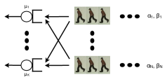
Figure 2: Arrivals from multiple populations into multiple queues.

The following Lemma shows an interesting self-organization property at equilibrium.

Lemma 4.1

Suppose that $\gamma_{1}<\gamma_{2}\cdots<\gamma_{N}$. Then, at equilibrium population $i$ users arrive before population $j$ users for $i<j$. Furthermore, the arrivals are over disjoint intervals, without any gaps.

Proof: Let $T_{s,k}=0$, for all queues $k$. The general case will follow easily from the ensuing argument. First note that there can be no gaps in any equilibrium arrival profile, $F_{k}=\sum_{i=1}^{N}F_{i,k}$. If there were, then, any arriving non-atomic user right after the gap can arbitrarily improve its cost by arriving just before such a gap, implying this arrival profile is not in equilibrium. Now, the cost of arriving at queue $k$ is constant, for a given population $i$ over the arrival interval. Differentiating $C_{i,k}(t)$, we have $0=(\alpha_{i}+\beta_{i})(\frac{1}{\mu_{k}}\frac{\partial F_{i,k}(t)}{\partial t})-\alpha_{i}.$ Solving the equation for $f_{i,k}$, the arrival density, we have $f_{i,k}(t)=\mu_{k}\gamma_{i}$.

Now, let $(t_{1},t_{3})$ be an arbitrary interval, and suppose that $t_{1}<t_{2}<t_{3}$, such that some population $j$ users arrive in $(t_{1},t_{2}]$ and only population $i$ users arrive in $(t_{2},t_{3})$. Consider the cost of arrival for population $j$, $C_{j,k}(t)=(\alpha_{j}+\beta_{j})\frac{F_{k}(t)}{\mu_{k}}-\alpha_{j}t$, for $t\in(t_{1},t_{3})$. As $(t_{1},t_{2}]$ is in the support of $F_{j,k}$, it follows that the cost of arrival is constant over this interval, and it can be evaluated at $t_{2}$. Now, let $\epsilon>0$ be small enough so that $t,t+\epsilon\in(t_{2},t_{3})$. Evaluating the cost of arrival at these points and taking the difference of the resulting expressions we obtain $C_{j,k}(t+\epsilon)-C_{j,k}(t)=(\alpha_{j}+\beta_{j})\left(\frac{\sum_{l=1}^{N}F_{l,k}(t+\epsilon)-\sum_{l=1}^{N}F_{l,k}(t)}{\mu_{k}}\right)-\alpha_{j}\epsilon.$ By assumption, there are only arrivals from population $i$ in the sub-interval $(t_{2},t_{3})$, and it follows that $F_{l,k}(t+\epsilon)=F_{l,k}(t)$ for all $l\neq i$. This implies that $C_{j,k}(t+\epsilon)-C_{j,k}(t)=(\alpha_{j}+\beta_{j})\frac{(F_{i,k}(t+\epsilon)-F_{i,k}(t))}{\mu_{k}}-\alpha_{j}\epsilon.$ Divide through by $\epsilon$ and let $\epsilon\rightarrow 0$ to obtain $C^{{}^{\prime}}_{j,k}(t)=(\alpha_{j}+\beta_{j})\frac{f_{i,k}(t)}{\mu_{k}}-\alpha_{j},$ where $f_{i,k}(t)$ is the density of the arrival profile $F_{i,k}(t)$, which was shown to be $f_{i,k}(t)=\mu_{k}\gamma_{i}$, for $t\in(t_{2},t_{3})\subset\text{Supp}F_{i,k}$. Substituting for $f_{i,k}$ it follows that $C^{{}^{\prime}}_{j,k}(t)=(\alpha_{j}+\beta_{j})(\gamma_{i}-\gamma_{j}).$ By assumption, $\gamma_{i}<\gamma_{j}$, so that $C^{{}^{\prime}}_{j,k}(t)<0$. This implies that the cost of arrival for population $j$ is strictly decreasing over the interval $(t_{2},t_{3})$, and it must be less than $C_{j,k}(t_{2})$. Clearly, $(t_{1},t_{2}]$ cannot be in the support of $F_{j,k}$ in equilibrium. This implies that population $j$ cannot arrive before population $i$, if $i<j$.   

4.1 Arrival Distribution

Figure 3: Two parallel queues, and two arriving populations with $\gamma_{1}<\gamma_{2}$. Population $1$ arrives over $[-T_{0,1},T_{1}]$ at queue 1, and over $[-T_{0,2},T_{1}]$ at queue 2. However, population $1$ need not be served completely until time $\tau_{1}$ at either queue. Population 2 arrives over $[T_{1},T_{2}]$ and is completely served at time $T_{2}$.

Denote by $-T_{0,k}$, the time of first arrival into queue $k$, and $T_{0}:=-T_{0,1}$, the time of the very first arrival to the network. Then, from Lemma 4.1, users from population $i$ arrive in the interval $[T_{i-1},T_{i}]$. Let $\tau_{i}$ denote the time the last user of population $i$ is served, and $\tau_{0}=0$. Obviously, $T_{i}\leq\tau_{i}$, with equality only if $i=N$ since at equilibrium the last (non-atomic) user to arrive into the network has no incentive to arrive before his service time. Figure 3 provides a simple illustration of this phenomenon, for two arriving populations at two parallel nodes.

Define $J_{i}=\{1\leq k\leq K:T_{s,k}\in[\tau_{i-1},\tau_{i}]\}$. Then, population $i$ users are served by the queues $\mathcal{J}_{i}=\bigcup_{j=1}^{i}J_{j}$, where queues $J_{i}$ first serve population $i$ before any other. Consider $l\in J_{i}$ with aggregate arrival profile $F_{l}(t)=\sum_{n=i}^{N}F_{n,l}(t)$, where by Lemma 4.1, $F_{n,l}$ has support $[T_{n-1},T_{n}]$. Note that $\sum_{l\in\mathcal{J}_{i}}p_{i,l}=\sum_{j=1}^{i}\sum_{k\in J_{j}}p_{i,k}=1$. We can now derive the equilibrium arrival profile for each population.

Theorem 4.2

Suppose $\gamma_{i}<\gamma_{i+1}$, $\forall i$ and $T_{s,k}<T_{s,k+1}$, $\forall k$. Then, the unique equilibrium arrival profile for population $i$ at queue $k\in J_{j}$, $j<i$, is $dF^{*}_{i,k}(t)=\gamma_{i}\mu_{k},\quad\forall t\in[T_{i-1},T_{i}]$, and at queue $l\in J_{i}$ is $dF^{*}_{i,l}(t)=\gamma_{i}\mu_{l}\quad\forall t\in[-T_{0,l},T_{i}]$ where $T_{N}=\frac{1}{\sum_{i=1}^{N}\sum_{k\in J_{i}}\mu_{k}}\left(N+\sum_{i=1}^{N}\sum_{k\in J_{i}}\mu_{k}T_{s,k}\right)$, and $T_{i-1}=T_{i}-\frac{p_{i,k}}{\gamma_{i}\mu_{k}}$ for $i=1,\cdots,N-1$, $k\in J_{j}$ and $j<i$. For $l\in J_{i}$, the arrival interval is $[-T_{0,l},T_{i}]$, where $-T_{0,l}=T_{i}-\frac{p_{i,l}}{\gamma_{i}\mu_{l}}$.

Furthermore, equilibrium routing probability for $l\in J_{i},i\geq 1$ is

$$p_{i,l}=\frac{\mu_{l}}{\sum_{j=1}^{i}\sum_{k\in J_{j}}\mu_{k}}\bigg{(}i-\sum_{j=1}^{i}\sum_{k\in J_{j}}\mu_{k}(T_{s,l}-T_{s,k})\bigg{)},$$ (9)

and for $k\in J_{j}$, $j<i$, and $i\geq 2$ is

$$p_{i,k}=\frac{\mu_{k}}{\sum_{j=1}^{i}\sum_{k\in J_{j}}\mu_{k}}\bigg{(}1-\sum_{l\in J_{i}}\frac{\mu_{l}}{\mu_{k}}(\sum_{q=j}^{i-1}p_{q,k})-\sum_{l\in J_{i}}\mu_{l}(T_{s,k}-T_{s,l})\bigg{)}.$$ (10)

Proof: Note that population $i$ is served by queues $J_{l},l\leq i$. The expected cost for a population $i$ user to arrive at queue $k\in\mathcal{J}_{i}$ is $C_{i,k}(t)=(\alpha_{i}+\beta_{i})W_{k}(t)+\beta_{i}t$ for $t\in[T_{i-1},T_{i}]$ for $k\in J_{l},l<i$ , and for $t\in[-T_{0,k},T_{i}]$ for $k\in J_{i}$. Recall that, $F_{k}(t)=\sum_{j=i}^{N}F_{j,k}(t)$, where $F_{i,k}(t)$ has support $[-T_{0,k},T_{i}]$ and $F_{jk}(t)$ has support $[T_{j-1},T_{j}]$ for each $j>i$. The virtual waiting time process at queue $k$ is given by $W_{k}(t)=\frac{1}{\mu_{k}}F_{k}(t)-(t-T_{s,k})$.

Now, note that at equilibrium, the expected cost for a population $i$ user to arrive at any queues $k,l\in J_{i}$ has to be the same. Thus, from $C_{i,k}(T_{i})=C_{i,l}(T_{i})$, we get that

$$\frac{p_{i,k}}{\mu_{k}}+T_{s,k}=\frac{p_{i,l}}{\mu_{l}}+T_{s,l}.$$ (11)

Let $p\leq q<i$ be two populations that arrive prior to population $i$. Then, for any $k\in J_{p}$ and $m\in J_{q}$, $k<m$ and at equilibrium the expected cost of arriving into queues $k$ and $m$ for a population $i$ user has to be the same. Thus, from $C_{i,k}(T_{i})=C_{i,m}(T_{i})$, we get

$$\frac{1}{\mu_{k}}(p_{p,k}+p_{p+1,k}+\cdots+p_{i,k})+T_{s,k}=\frac{1}{\mu_{m}}(p_{q,m}+p_{q+1,m}+\cdots+p_{i,m})+T_{s,m}.$$ (12)

First, consider $p<q$. Then, for a population $q$ user, $C_{q,k}(T_{q})=C_{q,m}(T_{q})$ for queues $k,m$ as above, which yields $\frac{1}{\mu_{k}}(p_{p,k}+p_{p+1,k}+\cdots+p_{i,k})+T_{s,k}=\frac{1}{\mu_{m}}(p_{q,m})+T_{s,m}$. Substituting this into (12) we have, by induction that

$$\frac{p_{i,m}}{\mu_{m}}=\frac{p_{i,k}}{\mu_{k}},\quad\forall k\in J_{p},~{}m\in J_{q},~{}p<q<i.$$ (13)

Now consider $p=q$. Then, for any $k,l\in J_{p}$ we have $C_{i,k}(T_{i})=C_{i,l}(T_{i})$, implying $\frac{1}{\mu_{k}}(p_{p,k}+\cdots+p_{i,k})+T_{s,k}=\frac{1}{\mu_{l}}(p_{p,l}+\cdots+p_{i,l})+T_{s,l}$. It follows from (11) that $\frac{p_{p,k}}{\mu_{k}}+T_{s,k}=\frac{p_{p,l}}{\mu_{l}}+T_{s,l}$. Thus, by induction, we have

$$\frac{p_{i,l}}{\mu_{l}}=\frac{p_{i,k}}{\mu_{k}},\quad\forall k,l\in J_{p},~{}p<i.$$ (14)

Next, let population $j<i$, and $k\in J_{j}$ and $l\in J_{i}$ are two queues that serve population $i$. Once again by the equilibrium conditions we have $C_{i,k}(T_{i})=C_{i,l}(T_{i})$. Simplifying the expression we obtain

$$p_{i,k}=\frac{\mu_{k}}{\mu_{l}}p_{i,l}+\mu_{k}(T_{s,l}-T_{s,k})-\sum_{p=j}^{i-1}p_{p,k}.$$ (15)

Now, we have $\sum_{p=1}^{i}\sum_{m\in J_{p}}p_{i,m}=1.$ Consider a $j<i$ and a $k\in J_{j}$ for $i\geq 2$. It follows that $\sum_{p=1,p\neq j}^{i}\sum_{m\in J_{p}}p_{i,m}+\sum_{l\in J_{j},l\neq k}p_{i,l}=1-p_{i,k}$. Substituting for $p_{i,m}$ and $p_{i,l}$ in terms of $p_{i,k}$ from (13), (14) and (15), we get $p_{i,k}$ in (10). Now, for an $l\in J_{i}$ for any $i\geq 1$, using (11) and (15) and substituting for $p_{i,k}$ and $p_{i,m}$ (respectively) in terms of $p_{i,l}$ in $\sum_{j=1}^{i-1}\sum_{m\in J_{j}}p_{i,m}+\sum_{k\in J_{i},k\neq l}p_{i,k}=1-p_{i,l}$, we get $p_{i,l}$ in (9).

We now derive the equilibrium arrival distributions for each population to each serving queue. First, recall that the cost function for population $i$ at queue $k\in J_{j},j<i$, is given by $C_{i,k}(t)=(\alpha_{i}+\beta_{i})\left(\frac{1}{\mu_{k}}F_{k}(t)+T_{s,k}\right)-\alpha_{i}t$ $\forall t\in[T_{i-1},T_{i}].$ Differentiating this and recalling that at equilibrium the cost is constant over the arrival interval, and that $F_{k}(t)=\sum_{p=j}^{i-1}p_{p,k}+F_{i,k}(t)$, we have $dF_{i,k}(t)=\gamma_{i}\mu_{k}\quad\forall t\in[T_{i-1},T_{i}]$. Now, for queue $k\in J_{i}$, the users arrive over the interval $[-T_{0,k},T_{i}]$. Again, differentiating the cost function $C_{i,k}(t)$, we have $dF_{i,k}(t)=\gamma_{i}\mu_{k}\quad\forall t\in[-T_{0,k},T_{i}]$.

Finally, we can derive the support of these distributions by backward recursion. Note that for population $N$, $\forall k\in J_{N}$ $\mu_{k}(T_{N}-T_{s,k})=p_{N,k}$. Substituting for $p_{N,k}$ from (11), we get $T_{N}=\left(N+\sum_{j=1}^{N}\sum_{k\in J_{j}}\mu_{k}T_{s,k}\right)/\left(\sum_{j=1}^{N}\sum_{k\in J_{j}}\mu_{k}\right)$.

Next, at equilibrium, we must have $C_{i,k}(T_{i})=C_{i,k}(T_{i-1})$ $\forall k\in J_{j},j<i$, from which we get $T_{i-1}=T_{i}-\frac{p_{i,k}}{\gamma_{i}\mu_{k}}.$ Note that we need to use $j<i$ in order to obtain the recursive definition of $T_{i-1}$, since $C_{i,k}(t)<C_{i,l}(t)$ on $[T_{i-1},-T_{0,l}]$, for $l\in J_{i}$; that is, there are no arrivals from population $i$ at queue $l\in J_{i}$ on this sub-interval. Finally, population $i$ users arrive at queue $k\in J_{i}$ in the interval $[-T_{0,l},T_{i}]$. Thus, at equilibrium we must have $C_{i,k}(-T_{0,k})=C_{i,k}(T_{i})$, from which we obtain $-T_{0,k}=T_{i}-\frac{p_{i,k}}{\gamma_{i}\mu_{k}}$.

The proof of uniqueness now follows that of Theorem 3.4 and we omit it for brevity.   

Remarks. 1. Theorem 4.2 shows that at equilibrium the arriving populations self-organize in ascending order of $\gamma_{i}$ and there are no gaps in the arrival profile. Further, the queues operate at full capacity till all arriving users have been served.

4.2 Price of Anarchy

We now compute the price of anarchy for the multiple populations case. Define the social cost at equilibrium with arrival profile $F$, as $J(F)=\sum_{i=1}^{N}J_{i}(F)$, where $J_{eq,i}=\sum_{j=1}^{i-1}\sum_{k\in J_{j}}\int_{T_{i-1}}^{T_{i}}C_{i,k}(t)dF_{i,k}(t)+\sum_{l\in J_{i}}\int_{-T_{0,l}}^{T_{i}}C_{i,l}(t)dF_{i,l}(t)$.

At equilibrium, the cost of arrival for population $i$ is uniform over the support of its arrival profile, and moreover is the same at all queues that the population chooses to arrive at. Thus, $C_{i,l}(t)=c_{i}$, some constant. Then, if $F$ is an equilibrium arrival profile $J_{eq,i}=c_{i}\left(\sum_{j=1}^{i-1}\sum_{k\in J_{j}}\int_{T_{i-1}}^{T_{i}}dF_{i,k}(t)+\sum_{l\in J_{i}}\int_{-T_{0,l}}^{T_{i}}dF_{i,l}(t)\right)=c_{i}\sum_{j=1}^{l}\sum_{k\in J_{j}}p_{0,k}=c_{i},$ since $\sum_{j=1}^{i}\sum_{k\in J_{j}}p_{0,k}$ = 1. The aggregate equilibrium social cost is given by $J_{eq}=\sum_{i=1}^{N}J_{eq,i}=\sum_{i=1}^{N}c_{i}$.

Let $e_{1}(i)$ denote the “first” queue in $J_{i}$, i.e., the queue with the earliest service start time $T_{s,l}$, $l\in J_{i}$. At equilibrium we have $C_{i,e_{1}(i)}(T_{i})\,=\,(\alpha_{i}+\beta_{i})(\frac{p_{i,e_{1}(i)}}{\mu_{e_{1}(i)}}+T_{s,e_{1}(i)})-\alpha_{i}T_{i}\,\equiv\,c_{i}$, where, $p_{i,e_{1}(i)}$ is the fraction of population $i$ users routed to queue $e_{1}(i)$. Now, let $e_{1}(1)$ be the very first queue to start service (and serve population 1 first). Without loss of generality, let $T_{s,e_{1}(1)}=0$. For population $i$ the cost of arrival at any queue in $\mathcal{J}_{i}$ is the same over the arrival interval, and it follows that $C_{i,e_{1}(i)}(T_{i})=C_{i,e_{1}(1)}(T_{i})$, which implies that $\frac{p_{i,e_{1}(i)}}{\mu_{e_{1}(i)}}+T_{s,e_{1}(i)}=\sum_{j=1}^{i}\frac{p_{j,e_{1}(1)}}{\mu_{e_{1}(1)}}$. Further, using the recursive definition of $T_{i}$, $T_{i}\,=\,T_{N}-\sum_{j=i+1}^{N}\frac{p_{j,e_{1}(1)}}{\gamma_{j}\mu_{e_{1}(1)}}$. Substituting for $\frac{p_{i,e_{1}(i)}}{\mu_{e_{1}(i)}}+T_{s,e_{1}(i)}$ and $T_{i}$ in $C_{i}(T_{i})$, we obtain

$$J_{eq}=\sum_{j=1}^{N}\alpha_{j}\bigg{(}\frac{1}{\gamma_{i}}\bigg{(}\sum_{j=1}^{i}\frac{\mu_{e_{1}(i)}}{\mu_{e_{1}(1)}}p_{j,e_{1}(1)}\bigg{)}-\mu_{e_{1}(i)}T_{s,e_{1}(i)}-\bigg{(}T_{N}-\sum_{j=i+1}^{N}\frac{p_{j,e_{1}(1)}}{\gamma_{j}\mu_{e_{1}(1)}}\bigg{)}\bigg{)}.$$ (16)

Now, from Theorem 4.2 we have an expression for $T_{N}$ in terms of the exogeneous parameters of the network. Substituting that into (16) we obtain an expression for $J_{eq}$ that is, unfortunately, quite messy for the general case. Below, we illustrate this expression for a much simpler special case.

Next, we note that the optimal arrival profile would be for each non-atomic user to arrive right at the instant of service. In this case, there is no waiting time and the cost of arrival at time $t$ is $\beta_{i}t$, for a user of population $i$. Let $\pi:\mathcal{N}\rightarrow\mathcal{N}$ be a permutation on the set of populations such that $\beta_{\pi(1)}>\cdots>\beta_{\pi(N)}$. In the optimal arrival profile populations should arrive in the order $\pi(1),\pi(2),\cdots,\pi(N)$.

A key observation is that since the sizeof each population is the same, the set of queues $\mathcal{J}_{i}$ that serve population $i$ at equilibrium, will now serve population $\pi(i)$. Let $\mathcal{J}^{*}_{i}$ be the set of queues that serve population $\pi(i)$ in the optimal arrival profile. This is because there are no gaps in the optimal and equilibrium arrival profiles. Thus, for given queue start time times, $T_{s,k}$, if population $i$ in the equilibrium arrival profile is replaced by population $\pi(i)$, the set of queues that served population $i$ will now serve population $\pi(i)$, whose users now arrive over $[T_{i-1},T_{i}]$, which is the equilibrium arrival interval for population $i$.

Thus, the optimal social cost is

$$J_{opt}=\sum_{i=1}^{N}J_{opt,\pi(i)}=\frac{1}{2}\sum_{i=1}^{N}\beta_{\pi(i)}\bigg{(}\sum_{j=1}^{i-1}\sum_{k\in J_{j}}\mu_{k}((T_{i}^{*})^{2}-(T_{i-1}^{*})^{2})+\>\sum_{l\in J_{i}}\mu_{l}((T_{i}^{*})^{2}-T_{s,l}^{2})\bigg{)},$$ (17)

where $T_{i}=\frac{i+\sum_{j=1}^{i}\sum_{k\in J_{j}}\mu_{k}T_{s,k}}{\sum_{j=1}^{i}\sum_{k\in J_{j}}\mu_{k}}$, and this is precisely the time at which population $i$ finishes service at equilibrium. We can substitute for $T_{i}$ in (17), which yields a fairly complicated expression for $J_{opt}$ and the price of anarchy, $\eta=J_{eq}/J_{opt}$, in terms of the exogeneous parameters.

To get some insight into the price of anarchy, $\eta$, we illustrate it for a special case where the service rate offered by every queue is the same $\mu>0$ and the start time of the $k$th queue is $\tau(k-1)$, for some $\tau>0$. Let the number of queues that serve the first $l$ populations to arrive be $K_{l}$. Then, the instant at which population $\pi(l)$ (or population $l$, at equilibrium) is served out is given by $T_{l}=\frac{l+\sum_{k=1}^{K_{l}}\mu\tau(k-1)}{\sum_{k=1}^{l}\mu}=\frac{l+\frac{\mu\tau}{2}K_{l}(K_{l}-1)}{\mu K_{l}}$. Note that $K_{l}$ is unknown a priori, but can be easily calculated. Suppose $\mu\tau<1$, and relax $K_{l}\in[1,K]$ to take real values. Then, the following Lemma shows that $T_{l}$ is a convex function of $K_{l}$. The optimal value of $K_{l}$ then is the nearest integer to the optimal real value computed. Let $[x]$ denote the nearest integer to the real number $x$.

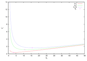
Figure 4: Terminal arrival time $T_{l}$ as a function of $K_{l}$, the number of queues that service population $l$, plotted for $l=1,7,14$, and for $\mu\tau=0.1$ and $\mu=1.0$.

Figure 4 plots $T_{l}$ as a function of $K_{l}$, the number of queues that serve population $l$. Note that $T_{l}$ is a convex function of $K_{l}$ and has a minima. We establish this fact formally in Lemma 4.3.

Lemma 4.3

Suppose $\mu\tau<1$. Then, $T_{l}$ is a convex function of $K_{l}\in(1,K]$. Further, it achieves a minimum at $K^{*}_{l}=[\sqrt{\frac{2l}{\mu\tau}}]$.

Proof: From Theorem 4.2 we have $T_{l}(k)=\frac{l}{\mu k}+\frac{\tau}{2}(k-1)$, for $k\in(1,K]$. Differentiating with respect to $k$ we obtain $\frac{\partial T_{l}(k)}{\partial k}=-\frac{l}{\mu k^{2}}+\frac{\tau}{2},$ which yields a critical point $k^{*}=\sqrt{2l/\mu\tau}$ (only the positive value is feasible). Further, the second derivative yields $\frac{\partial^{2}T_{l}(k)}{\partial k^{2}}=\frac{2l}{\mu k^{3}}>0\quad\forall k\in(1,K]$. Thus, $T_{l}(k)$ is convex for real $k$ and achieves its minimum at $K_{l}^{*}=[k^{*}]$.   

Remarks. 2. Lemma 4.3 shows that the number of queues that will serve population $l$, $K_{l}$, is proportional to $\sqrt{l}$, when $\mu\tau<1$.
3. If $(l-1)\leq\mu\tau<l$, then, there will be more than one queue that serves population $l$, and at most one that serves all populations with index less than $l$. In this case as well, the number of queues that serve population $l$ can be found by solving a convex optimization problem.

Now, we characterize the price of anarchy in the special case when every queue in the network serves at the same rate, and service start times are equi-spaces.

Theorem 4.4

Suppose that each queue offers the same service rate $\mu>0$, and queue $k$ starts service at time $\tau(k-1)$ with $\tau>0$. Then, the price of anarchy $\eta$ is

$$\eta=\frac{\frac{\tau}{2}\{(1-\frac{1}{\gamma_{N}})\sum_{l=1}^{N}\alpha_{l}+\sum_{l=1}^{N}\beta_{l}\}}{\frac{\mu}{2}\sum_{l=1}^{N}\beta_{l}\bigg{\{}\frac{\tau^{2}}{12}\sqrt{\frac{2}{\mu\tau}}(\sqrt{l}-\sqrt{l-1})+\frac{2\tau^{2}}{3}(\frac{2}{\mu\tau})^{3/2}(l\sqrt{l}-(l-1)\sqrt{l-1})-\frac{\tau}{\mu}\bigg{\}}}\leq 2.$$

Proof: The expression for $\eta$ follows by substituting, for any queue $l=1,\cdots,K$, $\mu_{l}=\mu$ and $T_{s,l}=\tau(l-1)$ (i.e., the queue $l$ starts service at time $\tau(l-1)$), in (16) and (17), using Lemma 4.3 and taking $K_{l}\approx\sqrt{2l/\mu\tau}$. The expression in the statement then follows after some elementary algebra and is omitted for brevity.

To see that $\eta$ is upper-bounded by 2, first consider $N=3$. The expression for $J_{opt}$ reduces to

$$J_{opt}= \beta_{1} \frac{\tau}{2}\bigg{(}\frac{4}{3}\sqrt{\frac{2}{\mu\tau}}+\frac{\mu\tau}{12}\sqrt{\frac{2}{\mu\tau}}-1\bigg{)}+\frac{\mu}{2}\beta_{2}\bigg{(}\tau\sqrt{\frac{2\tau}{\mu}}\bigg{(}\frac{\sqrt{2}-1}{12}+\frac{4}{3\mu\tau}(2\sqrt{2}-1)\bigg{)}-\frac{\tau}{\mu}\bigg{)}$$

$$\>+ \frac{\mu}{2}\beta_{3}\bigg{(}\tau\sqrt{\frac{2\tau}{\mu}}\bigg{(}\frac{\sqrt{3}-\sqrt{2}}{12}+\frac{4}{3\mu\tau}(3\sqrt{3}-2\sqrt{2})\bigg{)}-\frac{\tau}{\mu}\bigg{)}.$$

$J_{eq}$ is simply $\frac{\tau}{2}\bigg{(}1-\frac{1}{\gamma_{3}}\bigg{)}\sum_{i=1}^{3}\alpha_{\pi(i)}+\frac{\tau}{2}\sum_{i=1}^{3}\beta_{\pi(i)}\equiv\frac{\tau}{2}\bigg{(}1-\frac{1}{\gamma_{3}}\bigg{)}\sum_{i=1}^{3}\alpha_{i}+\frac{\tau}{2}\sum_{i=1}^{3}\beta_{i}$. Using these expressions, we evaluate $2J_{opt}-J_{eq}=$

$$\frac{\tau}{2}\sum_{i=1}^{3}(\alpha_{i})\bigg{(}\frac{1}{\gamma_{3}}-1\bigg{)} + \beta_{1}\frac{\tau}{2}\bigg{(}\frac{4}{3}\sqrt{\frac{2}{\mu\tau}}+\frac{\mu\tau}{12}\sqrt{\frac{2}{\mu\tau}}-\frac{3}{2}\bigg{)}+\beta_{2}\bigg{(}\mu\tau\sqrt{\frac{2\tau}{\mu}}\bigg{(}\frac{\sqrt{2}-1}{12}+\frac{4}{3\mu\tau}(2\sqrt{2}-1)\bigg{)}-\frac{3\tau}{2}\bigg{)}$$

$$\>+ \beta_{3}\bigg{(}\mu\tau\sqrt{\frac{2\tau}{\mu}}\bigg{(}\frac{\sqrt{3}-\sqrt{2}}{12}+\frac{4}{3\mu\tau}(3\sqrt{3}-2\sqrt{2})\bigg{)}-\frac{3\tau}{2}\bigg{)}.$$

The first term on the right hand side is $>0$, since $\gamma_{3}<1$ and $\alpha_{i}\geq 0$ for all $i$. The terms after $\beta_{2}$ and $\beta_{3}$ can easily be verified to be non-negative. The only term left to consider is the one after $\beta_{1}$. Denote $\delta=\frac{4}{3}\sqrt{\frac{2}{\mu\tau}}+\frac{\mu\tau}{12}\sqrt{\frac{2}{\mu\tau}}-\frac{3}{2}$. Multiplying and dividing by $\sqrt{2/\mu\tau}$ we have $\delta=\sqrt{\frac{\mu\tau}{2}}\left(\frac{4}{3}\frac{2}{\mu\tau}+\frac{1}{6}-\frac{3}{2}\sqrt{\frac{2}{\mu\tau}}\right)$. Let $x:=\sqrt{2/\mu\tau}$. Then, it can be seen that $\delta x=(\frac{4}{3}x^{2}-\frac{3}{2}x+\frac{1}{6})$. Suppose that $\delta x<0$. That is, (after factoring the LHS) $(8x-1)(x-1)<0$. This implies either $(8x-1)>0$ and $(x-1)<0$, which contradicts the fact that $x=\sqrt{2/\mu\tau}>1$ when $\mu\tau<1$; or $(8x-1)<0$ and $(x-1)>0$ which is impossible. Therefore, it cannot be the case that $(8x-1)(x-1)<0$, thus proving that $2\geq J_{eq}/J_{opt}$. It can also be checked (after some tedious algebra) that the terms after $\beta_{l}$, for $l>3$, are larger than those after $\beta_{3}$ and so it is possible to use the same argument for an arbitrary number of arriving populations, $N$.   

5 Exact equilibrium analysis: An example with two users

A natural question is whether equilibria can be found in a finite population strategic arrival game, and how close the non-atomic equilibrium is to such an outcome. It turns out that finite population equilibrium analysis is not malleable to a tractable analysis in general, and the resulting expressions can be solved exactly only in some special cases. We illustrate the methodology with two FIFO queues serving in parallel, with two arriving users, with service rates $\mu_{k}$, service start times $T_{s,1}=T_{s,2}=0$. We derive the exact equilibrium arrival distribution, and show that it is unique. The extension to more than two users cannot be solved in closed form. Finite population analysis for a single server queue can be found in Juneja and Shimkin (2011), which also makes the same observation.

Let the two users be indexed by $i\in\{1,2\}$, and let $T_{i}$ be the arrival time of user $i$. Assume that the distribution function $F_{i}$ of $T_{i}$ is absolutely continuous. Let $\xi_{i}(t)=k\in\{1,2\}$ be a routing random variable, such that $\xi_{i}(\omega,t)=k$ implies that user $i$ at time $t$ is routed to queue $k$. Let $p_{i,k}(t):=P(\xi_{i}(t)=k)$ be the probability of user $i$ being routed to queue $k$ at time $t$. Let $Q^{i}_{k}(t)$ be the number of other arrivals that user $i$ observes in queue $k$ at time $t$, and let $A^{i}_{k}(t)$ denote the aggregate number of arrivals, other than the user $i$, to queue $k$ queue by time $t$, and let $S_{k}(t)$ denote the cumulative number of (potential) service completions, at queue $k$, up to time $t$.

As noted before, the path-wise description of the queue length process is given by $Q^{i}_{k}(t)=(A^{i}_{k}(t)-S_{k}(t))_{+},\quad t\in\mathbb{R},\quad i\in\{1,2\}~{}\text{and}~{}k\in\{1,2\}$. We also make the assumption that the routing, arrival and service processes are mutually independent. We denote by $-i$, the user $j\neq i$. The following proposition describes the dynamics of the expected queue length, $\bar{Q}^{i}_{k}(t)$.

Proposition 5.1

$\bar{Q}^{i}_{k}(t+dt)=\bar{Q}^{i}_{k}(t)+p_{k}(t)f_{-i}(t)dt-\mu_{k}(1-P_{k,0}(t))dt\mathbf{1}_{\{t\geq 0\}}\quad\forall i\in\{1,2\}\text{ and }k\in\{1,2\},$ where, $f_{-i}(\cdot)$ is the density function of the arrival time of the user other than user $i$ and $P_{k,0}(t)$ is the probability that the queue $k$ is empty at time $t$, i.e., $P_{k,0}(t)=P(Q^{i}_{k}(t)=0)$.

Proof: It is easy to see that $\bar{Q}^{i}_{k}(t+dt)=\bar{Q}^{i}_{k}(t)+\mathbb{E}[A^{i}_{k}(t+dt)-A^{i}_{k}(t)]-\mathbb{E}[D_{k}(t+dt)-D_{k}(t)]\mathbf{1}_{\{t\geq 0\}}$. Here, $D_{k}(t)$ is the number of actual service completions by time $t$ and $\mathbb{E}[A^{i}_{k}(t+dt)-A^{i}_{k}(t)]$ is the expected number of users other than $i$ who might arrive in the interval $[t,t+dt]$. The expectation of user $-i$ arriving in an infinitesimal time interval is $p_{k}(t)f_{-i}(t)dt$. The expected number of service completions in the interval $[t,t+dt]$ is given simply by $\mu_{k}(1-P(Q^{i}_{k}(t)=0))dt$. The expression for $\bar{Q}^{i}_{k}(t)$ follows by substitution.   
The mean virtual waiting time of user $i$ at queue $k$ at time $t$ is given by $\bar{W}^{i}_{k}(t)=\frac{\bar{Q}_{k}^{i}(t)}{\mu_{k}}-t\mathbf{1}_{\{t\leq 0\}}$. Note that an arrival at time $t<0$, would have to wait for $t$ units of time before service commences, explaining the presence of the term $t\mathbf{1}_{\{t\leq 0\}}$.

Now, users choose a mixed strategy over the arrival interval and the routing random variable. Thus, the strategy space of the game is $\mathcal{C}_{b}\times[0,1]^{2}$, where $\mathcal{C}_{b}$ is the space of non-decreasing and absolutely continuous functions with support in $\mathbb{R}$, and $[0,1]^{2}$ is the set that the routing probabilities take values in. Thus, user $i$ chooses the tuple $(F_{i},\mathbf{p}_{i})(t),~{}\forall t\in\mathbb{R}$, where $\mathbf{p}_{i}(t)=(p_{1,i}(t),p_{2,i}(t))^{{}^{\prime}}$ is a vector of probabilities at time $t$. Thus, the choice of $\mathbf{p}_{i}(t)$ must satisfy the constraint $p_{1,i}(t)+p_{2,i}(t)=1$. We designate $\textbf{F}=(F_{1},F_{2})$ as an arrival profile and $\textbf{P}=(\mathbf{p}_{1},\mathbf{p}_{2})$ as a routing profile of the game. We are interested in symmetric equilibria in this one-shot arrival game, such that $F_{1}=F_{2}$ and $\mathbf{p}_{1}=\mathbf{p}_{2}$. For brevity, we drop the superscripts from $Q_{k}^{i}$ and $A_{k}^{i}$, as the definition should be clear from the context.

Now, as before, the expected cost of arriving at queue $k$ is a weighted sum of the waiting time and the time at which the user arrives, which yields $C_{k}(t)=(\alpha+\beta)\left(\frac{\bar{Q}_{k}(t)}{\mu_{k}}-t\mathbf{1}_{\{t\leq 0\}}\right)+\beta t$. Note that the equilibrium arrival profile will have some finite support $[-T_{0,k},T_{k}]$ for queue $k$ since the expected cost is increasing in both $t$ and $-t$ (since there is only one other user, the expected queue length is bounded by 1). Furthermore, the expected cost of arrival must be the same at either queue. If this were not the case, then an arriving user could improve its cost by choosing to arrive at a queue with a lower cost. We are interested in symmetric equilibria for which the arrival interval must be the same at either queue. Let this interval be $[-T_{0},T]$, where $-T_{0}$ and $T$ are determined in equilibrium.

Theorem 5.2

The equilibrium profile, ($\textbf{F}^{*},\textbf{P}^{*}$), of the strategic arrivals game with two users and two queues is given by

$$f^{*}(t)=\begin{cases}&\gamma(\mu_{1}+\mu_{2})\quad t\in[-T_{0},0]\\ &\gamma(\mu_{1}+\mu_{2})-\mu_{1}P_{1,0}(t)-\mu_{2}P_{2,0}(t)\quad t\in(0,T],\end{cases}$$

$$\quad\text{and}~{}~{}~{}p^{*}_{i}(t)\,=\,\begin{cases}&\frac{\mu_{i}}{(\mu_{1}+\mu_{2})},\quad t\in[-T_{0},0]\\ &\frac{\mu_{i}}{(\mu_{1}+\mu_{2})}+(\mathbf{1}_{\{i=1\}}-\mathbf{1}_{\{i=2\}})\frac{\mu_{1}\mu_{2}(\mu_{2}-\mu_{1})}{(\mu_{1}+\mu_{2})f(t)}\frac{\beta t}{(\alpha+\beta)},\quad t\in(0,T],\end{cases}$$

where $\gamma=\alpha/(\alpha+\beta)$, $P_{i,0}(t)=1-\frac{\mu_{i}(\beta t-\alpha T_{0})}{\alpha+\beta}$ and

$$T_{0}=-\bigg{(}\frac{\mu_{1}+\mu_{2}}{(\mu_{1}^{2}+\mu_{2}^{2})}\bigg{)}\sqrt{\bigg{(}2+\frac{\beta}{\alpha}\bigg{)}\frac{\beta}{\alpha}}\quad\text{ and }\quad T=\bigg{(}\frac{\mu_{1}+\mu_{2}}{\mu_{1}^{2}+\mu_{2}^{2}}\bigg{)}\bigg{(}\sqrt{\frac{2\alpha}{\beta}+1}-1\bigg{)}.$$

The proof can be found in the appendix.

Remarks. 1. Note that the general case of $K$ parallel queues serving $n$ users is not as simple as the result above. The network state dynamics are determined by a set of $K$ coupled differential equations, that are in general quite difficult to solve. Instead, using a fluid approximation reduces the complexity of the problem, by allowing one to replace the differential equations by simple linear equations.

2. The fluid analysis does lose some accuracy, however, for small numbers of arrivals since it suggests that queues can never be idle at equilibrium, but for a large number of users it still captures the essential features of the strategic arrivals game.

6 Conclusions

In this paper, we have presented three results. First, we have developed large population fluid approximations to various processes of interest in a parallel queueing network where the arriving users choose a time of arrival from an arbitrary distribution function. We believe these are entirely new results and should be of independent interest. Second, using this framework, we then studied the network concert queueing game in the large population regime. We proved the existence and uniqueness of the non-atomic equilibrium arrival profile, both in the case of a homogeneous population of users, as well as heterogeneous populations with disparate cost characteristics. In either case, we also characterized the price of anarchy of the game, due to strategic arrivals. Third, we demonstrated the methodology for finite population analysis, by analyzing a simple instance with two strategic users arriving at a two queue network, and deriving the equilibrium arrival profile.

The queueing model that we have introduced in this paper is of relevance in several settings including transportation networks, data center network traffic, etc. Thus, it would be useful to understand further the various stochastic processes. For example, the FSLLN/fluid limit analysis shows that at equilibrium, no queue is ever idle. This, however, cannot be true in the case of a finite population, where, as we have seen in Section 5, there is a positive probability of the queue being idle during the arrival interval. Thus, we must derive better approximations to the arrival, queue-length and waiting-time processes. One way would be to derive diffusion limits by developing functional central limit theorems (FCLT) for the queueing system model we introduced. This is a current line of our research. In particular, we have been able to establish that the diffusion limiting process to the queue-length in a single server queue is combination of a Brownian motion and a Brownian bridge, where the weak convergence has been established in Skorokhod’s $M_{1}$ topology.

Finally, the alternative queueing system model we have introduced in this paper may involve a general queueing network. In such a setting, it would be useful to develop the fluid and diffusion limits for the various processes of interest, and to establish the set of (non-atomic) strategic equilibria that result. We are currently working towards this goal. Our hope is that the framework that we have introduced would be of greater relevance for some scenarios, as well as more tractable than the GI/G/1 models in standard queueing theory.

Appendix

We first state two Lemmas that are useful in proving Theorem 2.1, and are also useful below.

Lemma 6.1

Let $A^{n}_{k}(t),\,\,\forall k$, be as defined in (1), where $n$ is the population size, and $\mathbf{p}=(p_{0,1},\cdots,p_{0,K})^{{}^{\prime}}$. Then, $\bar{A}^{n}(t):=\frac{A^{n}(t)}{n}\rightarrow F(t)\quad a.s.~{}u.o.c.~{}\forall t\in[-T_{0},T]$, as $n\rightarrow\infty$.

Lemma 6.2

Let $\bigg{(}\frac{1}{n}S_{k}^{n}(t),V_{k}^{n}(t+T_{0})\bigg{)}$ be as defined in (2) and (3), where $k\in\{1,\cdots,K\}$ and $t\in[-T_{0},\infty)$. Then, as $n\rightarrow\infty$,

$$\bigg{(}\frac{1}{n}\mathbf{S}^{n}(t),\mathbf{V}^{n}(t+T_{0})\bigg{)}\rightarrow(\bar{\mathbf{S}}(t),\bar{\mathbf{V}}(t)):=(\mathbf{M}^{-1}\mathbf{t_{s,+}}(t),\mathbf{M}\mathbf{1}(t+T_{0}))\quad a.s.~{}u.o.c.~{}\quad\forall\,t\in[-T_{0},\infty),$$

where $M:=diag(m_{1},\cdots,m_{K})$ is a diagonal matrix of the mean service times at each node, $\mathbf{t_{s,+}}(t):=((t-T_{s,1}))\mathbf{1}_{\{t\geq T_{s,1}\}},\cdots,(t-T_{s,K})\mathbf{1}_{\{t\geq T_{s,K}\}})^{{}^{\prime}}$ and $\mathbf{1}=(1,\cdots,1)^{{}^{\prime}}$.

Both Lemmas above can be proved easily using the Strong Law of Large Numbers, and their proofs are omitted due to space constraints.

Proof of Proposition 2.2

Proof: (Proposition 2.2) In order to establish a functional strong law of large numbers result for (4) we first require the following lemma relating the processes $\mathbf{I}_{k}^{n}(t):=\bigg{(}\int^{t}_{T_{s,k}}\mathbf{1}_{\{Q_{k}^{n}(s)=0\}}ds\bigg{)}\mathbf{1}_{\{t\geq T_{s,k}\}}$ and $\tilde{\mathbf{I}}^{n}(t):=\int^{t}_{-T_{0}}\mathbf{1}_{\{Q_{k}^{n}(s)=0\}}ds$.

Lemma 6.3

Let $I_{k}^{n}(t)$ and $\tilde{I}_{k}^{n}(t)$, the $k$th components of $\mathbf{I}^{n}(t)$ and $\tilde{\mathbf{I}}^{n}(t)$, be elements of $\mathcal{D}$. Then, as $n\rightarrow\infty$, $|I_{k}^{n}(t)-\tilde{I}_{k}^{n}(t)|\rightarrow 0\,\,a.s.\quad u.o.c.\,\,\forall t\in[-T_{0},\infty).$ Thus, $|\mathbf{I}^{n}(t)-\tilde{\mathbf{I}}^{n}(t)|\rightarrow 0,\,\,a.s.\quad u.o.c.\,\,\forall t\in[-T_{0},\infty)$.

The proof of Lemma 6.3 follows directly from the following result.

Lemma 6.4

Let $(\Omega,\mathcal{F},P)$ be a probability space. $F(t)$ is a distribution function of a random variable $\mathcal{T}$ on this space, with support $[S,T]\,\subset\mathbb{R}$. Assume that $F(t)$ is absolutely continuous. Suppose $T_{1},T_{2},\cdots,T_{n}$ are $n$ I.I.D. samples drawn from $\mathcal{T}$. Define $T_{1}^{(n)}:=\inf\{T_{1},T_{2},\cdots\,T_{n}\}$ as the value of the smallest sample. Then, it follows that, $T_{1}^{(n)}\downarrow S\quad a.s.\quad\text{ as }n\rightarrow\infty.$

Proof: We will prove this in the case of a uniformly distributed random variable, on $[0,1]$. Let $U(t)$ be the distribution function of the standard uniform random variable, and let $F(t)=U(t)$. The general case then follows by making use of a transformation of the uniform random variable, since $F(t)$ is assumed to be absolutely continuous. Fix $\epsilon>0$. Consider the event, $E_{n}\,:=\,\{\omega:T_{1}^{(n)}\geq\epsilon\}.$ The measure of this event is given by, $P(E_{n})\,=\,P(T_{1}^{(n)}\geq\epsilon)\,=\,P(\inf\{T_{1},\cdots,T_{n}\}\geq\epsilon).$ Since the samples are I.I.D., it follows easily that, $P(E_{n})=[P(T_{1}\geq\epsilon)]^{n}=[1-F(\epsilon)]^{n}.$ Since $F(t)$ is absolutely continuous, it follows that, $\sum_{n=1}^{\infty}P(E_{n})\,<\,\infty.$ By the First Borel- Cantelli Lemma, it follows that $P(T_{1}^{(n)}\geq\epsilon\,\,\,i.o.)=0$. This implies that $T_{1}^{(n)}\downarrow S=0\,\,a.s.$.   
Proof: (Lemma 6.3) Let $\tau>0$. As the queue is non empty after the very first arrival to the node, we have $I_{k}^{n}(t)\equiv(\int_{T_{k,1}^{(n)}}^{t}\mathbf{1}_{\{Q_{k}^{n}(s)=0\}}ds)\mathbf{1}_{\{t\geq T_{s,k}\}}$. It is easy to see that $I_{k}^{n}(t)\leq\tilde{I}_{k}^{n}(t)\quad\forall t\in[-T_{0},\tau]$. Also, $I_{k}^{n}(t)\geq\tilde{I}_{k}^{n}(t)-\int_{-T_{0}}^{T_{k,1}^{(n)}}\mathbf{1}_{\{Q_{k}^{n}(s)=0\}}ds,\quad\forall t\in[-T_{0},\tau]$. It follows that $\int_{-T_{0}}^{T_{k,1}^{(n)}}\mathbf{1}_{\{Q_{k}^{n}(s)=0\}}ds\,\geq\,\tilde{I}_{k}^{n}(t)-I_{k}^{n}(t)\,\geq\,0.$

The conclusion follows on $[-T_{0},\tau]$, by noting that $Q_{k}^{n}(s)=0\,\,\forall s\in[-T_{0},T^{(n)}_{k,1}]$ and applying Lemma 6.4. Since $\tau$ is arbitrary, the lemma is proved.   
Now, we can proceed to prove Lemma 2.2, and we analyze the claim component-wise, since the processes at each node are statistically independent. The result follows by applying Lemmas 6.1, 6.2 and 6.3 to (4). First, note that $B^{n}_{k}(t)\leq t$. Thus, by the Random Time Change Theorem (Theorem 5.5, Chen and Yao (2001)) and Lemma 6.2 it follows that $\frac{1}{n}S_{k}^{n}(B_{k}^{n}(t))-\mu_{k}B_{k}^{n}(t)\rightarrow 0,$ $\,\,a.s.\quad u.o.c.\text{ as }n\rightarrow\infty\,\,\forall t\in[-T_{0},\infty)$. By Lemma 6.1 we have $\frac{1}{n}A_{k}^{n}(t)-p_{0,k}F(t)\rightarrow 0,$ $\,\,a.s.\quad u.o.c.\text{ as }n\rightarrow\infty\,\,\forall t\in[-T_{0},\infty)$. Applying these results and Lemma 6.3 to (4) we have $X_{k}^{n}(t)\rightarrow\bar{X}_{k}(t):=(p_{0,k}F(t)-\mu_{k}(t-T_{s,k})\mathbf{1}_{\{t\geq T_{s,k}\}})\,\,a.s.\quad u.o.c.\,\,\text{ as }n\rightarrow\infty$. It follows that $\mathbf{X}^{n}(t)\rightarrow(\mathbf{p}F(t)-\mathbf{M}^{-1}\mathbf{t_{s,+}}(t)),$ $\,\,a.s.\quad u.o.c.,\text{ as }n\rightarrow\infty,\,\,\forall t\in[-T_{0},\infty)$.   

Proof of Theorem 2.3

Proof: Recall that $\frac{1}{n}\mathbf{Q}^{n}(t):=\mathbf{X}^{n}(t)+\mathbf{Y}^{n}(t)$, where $\mathbf{X}^{n}$ and $\mathbf{Y}^{n}$ are defined in (4) and (5), respectively. Note that if we defined $\mathbf{Y}^{n}(t):=\mathbf{I}^{n}(t)=\mathbf{t}_{s,+}(t)-\mathbf{B}^{n}(t)$, the Oblique Reflection Mapping Theorem (Theorem 7.2, Chen and Yao (2001)) would not be satisfied, since this process could be zero even when $\mathbf{Q}^{n}(t)$ is zero. To see this, note that if $T_{1}^{(n)}$ is the time of the first arrival to the network then, $\forall t\in[-T_{0},T_{1}^{(n)}]$, $\mathbf{I}^{n}(t)$ and $\mathbf{Q}^{n}(t)$ would be zero, violating the Oblique Reflection Mapping Theorem.

It is a simple exercise to verify that Theorem 7.2 of Chen and Yao (2001) is satisfied, in the case of a parallel node network, with $\mathbf{Y}^{n}(t)=\mathbf{M}^{-1}\tilde{\mathbf{I}}^{n}(t)$: The zero matrix $P$ is trivially a $M$-matrix. By definition, we have $\mathbf{Q}^{n}(t)\geq 0,\,\,\forall t\in[-T_{0},\infty)$. $\mathbf{Y}^{n}(t)$ is a non-decreasing $K$-dimensional process that only grows when every component of $\mathbf{Q}^{n}(t)$ is zero.

This implies, $(\frac{1}{n}\mathbf{Q}^{n}(t),\mathbf{Y}^{n}(t))=(\Phi(\mathbf{X}^{n}(t)),\Psi(\mathbf{X}^{n}(t))).$ The reflection regulator map, $\Psi(\cdot)$, is Lipschitz continuous under the uniform metric (Theorem 7.2, Chen and Yao (2001)). By the Continuous Mapping Theorem and Lemma 2.2 it follows that $(\Phi(\mathbf{X}^{n}(t)),\Psi(\mathbf{X}^{n}(t)))\rightarrow(\Phi(\bar{\mathbf{X}}(t)),\Psi(\bar{\mathbf{X}}(t))),\,\,a.s.\quad u.o.c.\text{ as }n\rightarrow\infty,\,\,\forall t\in[-T_{0},\infty).$   

Proof of Theorem 2.4

Proof: We prove the Theorem by treating the busy time and virtual waiting time processes separately. The fluid limit of the busy time process is derived in the following Lemma.

Lemma 6.5

Let $\mathbf{B}^{n}:=(B_{1}^{n},\cdots,B_{K}^{n})^{{}^{\prime}}$ be an element of $\mathcal{D}^{K}$. Then as $n\rightarrow\infty$ $\mathbf{B}^{n}(t)\rightarrow\bar{\mathbf{B}}(t):=\mathbf{t_{s,+}}(t)-\mathbf{M}\Psi(\bar{\mathbf{X}}(t))=\mathbf{t_{s,+}}(t)-\mathbf{M}\sup_{-T_{0}\leq s\leq t}[-\bar{\mathbf{X}}(s)]_{+}\,\,u.o.c.\,\,a.s.,\,\,\forall t\in[-T_{0},\infty),$ where, $\mathbf{t_{s,+}}(t)=(t\mathbf{1}_{\{t\geq T_{s,1}\}},\cdots,t\mathbf{1}_{\{t\geq T_{s,K}\}})^{{}^{\prime}}$ and $M=diag(m_{1},\cdots,m_{K}).$

Proof: By definition, we have, $\mathbf{B}^{n}(t)=\mathbf{t_{s,+}}(t)-\mathbf{I}^{n}(t).$ Adding and subtracting the vector process $\tilde{\mathbf{I}}^{n}(t)$ and noting that $\mathbf{Y}^{n}(t)=\mathbf{M}^{-1}\tilde{\mathbf{I}}^{n}(t)$ we have $\mathbf{B}^{n}(t)=\mathbf{t_{s,+}}(t)-\mathbf{M}\mathbf{Y}^{n}(t)+\tilde{\mathbf{I}}^{n}(t)-\mathbf{I}^{n}(t).$ Using Lemma 6.3 from the Appendix and Theorem 2.3 it follows that as $n\rightarrow\infty$, $\mathbf{B}^{n}(t)\rightarrow\mathbf{t_{s,+}}(t)-\mathbf{M}\Psi(\bar{\mathbf{X}}(t))\,\,a.s.\quad u.o.c.,\,\,\forall t\in[-T_{0},\infty).$   
Next, we derive the fluid limit of the virtual waiting time process in the following Lemma.

Lemma 6.6

Let $\mathbf{W}^{n}=(W_{1}^{n},\cdots,W_{K}^{n})^{{}^{\prime}}\in\mathcal{D}^{K}$. Then as $n\rightarrow\infty$ $\mathbf{W}^{n}(t)\rightarrow\bar{\mathbf{W}}(t):=\mathbf{M}\mathbf{p}F(t)-\bar{\mathbf{B}}(t)-\mathbf{t_{s,-}}(t)\quad a.s.\quad u.o.c.,\,\,\forall t\in[-T_{0},\infty),$ where $\mathbf{t_{s,-}}(t)=((t-T_{s,1})\mathbf{1}_{\{t\leq T_{s,1},\}},\cdots,(t-T_{s,K})\mathbf{1}_{\{t\leq T_{s,K}\}})^{{}^{\prime}}$, $\mathbf{p}=(p_{0,1},\cdots,p_{0,K})^{{}^{\prime}}$ and $\mathbf{M}=diag(m_{1},\cdots,m_{K})$.

Proof: The theorem follows by an application of Lemma 2.1, the Random Time Change Theorem (Theorem 5.5, Chen and Yao (2001)) and Lemma 2.4. We define the following vector for notational convenience. Let $\mathbf{V}(A(t)):=(V_{1}(A_{1}(t)),\cdots,V_{K}(A_{K}(t)))^{{}^{\prime}}$ The fluid-scaled version of the virtual waiting time process is given by $\mathbf{W}^{n}(t)=\mathbf{V}^{n}(A^{n}(t))-\mathbf{B}^{n}(t)-\mathbf{t_{s,-}}(t).$ First note that by Lemma 6.2 and the Random Time Change Theorem $\mathbf{V}^{n}(A^{n}(t))-\mathbf{M}\frac{1}{n}\mathbf{A}^{n}(t)\rightarrow 0\,\,u.o.c.\quad a.s.\text{ as }n\rightarrow\infty,\,\,\forall t\in[-T_{0},\infty)$. Thus, centering the process $\mathbf{V}^{n}(A^{n}(t))$ we get $\mathbf{W}^{n}(t)=\mathbf{V}^{n}(A^{n}(t))-\mathbf{M}\frac{1}{n}\mathbf{A}^{n}(t)+\mathbf{M}\frac{1}{n}\mathbf{A}^{n}(t)-\mathbf{B}^{n}(t)-\mathbf{t_{s,-}}(t).$ Applying Lemma 6.1, Lemma 2.4 and the comment above we have $\mathbf{W}^{n}(t)\rightarrow\mathbf{M}\mathbf{p}F(t)-\bar{\mathbf{B}}(t)-\mathbf{t_{s,-}}(t).$ Substituting for $\bar{\mathbf{B}}(t)$ we get $\bar{\mathbf{W}}(t)=\mathbf{M}\mathbf{p}F(t)-(\mathbf{t_{s,+}}(t)-\mathbf{M}\Psi(\bar{\mathbf{X}}(t)))-\mathbf{t_{s,-}}(t)=\mathbf{M}\bar{\mathbf{Q}}(t)-\mathbf{t_{s,-}}(t).$   

Proof of Theorem 5.2

Proof: Recall that $C_{i}(t)=c$, a constant,  $\forall i\in\{1,2\}$. Noting that that expected queue length at time $-T_{0}$ is zero, it is easy to see that $c=\alpha T_{0}$. It follows that $C^{{}^{\prime}}_{i}(t)=0$. Thus, solving for $p_{i}(t)f(t)$ we obtain

$$p_{i}(t)f(t)\,=\,\begin{cases}&\gamma\mu_{i}\quad t\in[-T_{0},0]\\ &\gamma\mu_{i}-\mu_{i}P_{i,0}(t)\quad t\in(0,T].\end{cases}$$

Using the fact that $p_{1}(t)+p_{2}(t)=1$, we solve for $p_{1}(t)$ and $p_{2}(t)$ to obtain

$$p_{i}(t)\,=\,\begin{cases}&\frac{\mu_{i}}{(\mu_{1}+\mu_{2})}\quad t\in[-T_{0},0]\\ &\frac{\mu_{i}}{(\mu_{1}+\mu+2)}+(\mathbf{1}_{\{i\equiv 1\}}-\mathbf{1}_{\{i\equiv 2\}})\frac{\mu_{1}\mu_{2}(\mu_{2}-\mu_{1})}{(\mu_{1}+\mu_{2})f(t)}\frac{\beta t}{(\alpha+\beta)}\quad t\in(0,T].\end{cases}$$

Thus, it can be seen that the probability of being routed to queue $i$ (in equilibrium) is constant before service commences, and is time dependent afterwards. The time dependence is determined by the expected idle time of the queue, as can be seen by solving for $f(t)$. Again, using the fact that $p_{1}(t)+p_{2}(t)=1$, add the equations for $p_{i}(t)f(t)$, for $i\in\{1,2\}$, to obtain

$$f(t)=\begin{cases}&\gamma(\mu_{1}+\mu_{2})\quad t\in[-T_{0},0]\\ &\gamma(\mu_{1}+\mu_{2})-\mu_{1}P_{1,0}(t)-\mu_{2}P_{2,0}(t)\quad t\in(0,T].\end{cases}$$

Interestingly, the arrival distribution is piecewise continuous. It is uniform up to time $0$, at which point service commences, and is a continuous function of $t$ in $[0,T]$. Notice that when there are only two arriving users, the expected queue length observed by one of the arrivals is fully determined by the probability of idling. We have for queue $i$, $\bar{Q}_{i}(t)=1\times P(Q_{i}(t)=1)+0\times P(Q_{i}(t)=0)=P_{i,1}(t).$ Now, using the fact that $P_{i,0}(t)+P_{i,1}(t)=1$ and the fact that $C_{i}(t)=\alpha T_{0}$, we can solve for $P_{i,1}(t)$ to obtain $P_{i,1}(t)=\frac{\mu_{i}(\beta t-\alpha T_{0})}{(\alpha+\beta)}=1-P_{i,0}(t).$ Thus, we can now substitute for $f(t)$ on $(0,T]$ to obtain $f(t)\,=\,(\gamma-1)(\mu_{1}+\mu_{2})+\frac{\alpha T_{0}-\beta t}{(\alpha+\beta)}(\mu_{1}^{2}+\mu_{2}^{2}).$

By definition, we have $\int_{-T_{0}}^{T}f(t)dt=1$. Note that $f(t)$ is a continuous function of $t$ in the interval $[0,T]$. By assumption, $F$ has no point masses. Thus, it follows that $f(T)=0$. Now, using the fact that $\int_{-T_{0}}^{T}f(t)dt=1$ we have $(\gamma-1)(\mu_{1}+\mu_{2})(T+T_{0})-(\mu_{1}^{2}+\mu_{2}^{2})((1-\gamma)\frac{T^{2}-T_{0}^{2}}{2}-\gamma T_{0}(T+T_{0}))=1.$ Next, using the fact that $f(T)=0$, we have $T=\frac{\mu_{1}+\mu_{2}}{\mu_{1}^{2}+\mu_{2}^{2}}-\frac{\alpha}{\beta}T_{0}.$ Substituting for $T$ in terms of $T_{0}$ from the expression above, and solving the resulting quadratic equation, we obtain

$$T_{0}=-\bigg{(}\frac{\mu_{1}+\mu_{2}}{(\mu_{1}^{2}+\mu_{2}^{2})}\bigg{)}\sqrt{\bigg{(}2+\frac{\beta}{\alpha}\bigg{)}\frac{\beta}{\alpha}}\quad\text{and}\quad T=\bigg{(}\frac{\mu_{1}+\mu_{2}}{\mu_{1}^{2}+\mu_{2}^{2}}\bigg{)}\bigg{(}\sqrt{\frac{2\alpha}{\beta}+1}-1\bigg{)}.$$

These expressions describe the symmetric equilibrium strategy $(F^{*},\textbf{p}^{*})$ in the case of two strategically arriving users and two parallel queues. The uniqueness of the equilibrium profile follows by construction. For given service rates and cost characteristics, it is clear that $T$ and $T_{0}$ are unique. It is easy to see that $T$ and $-T_{0}$ together fully determine $F^{*}$ and hence $\textbf{p}^{*}$. It follows that the arrival profile and routing profiles are unique.

References

- Adlakha and Johari (2010) Adlakha, S., R. Johari. 2010. Mean field equilibrium in dynamic games with strategic complementarities. Submitted .
- Billingsley (1968) Billingsley, P. 1968. Convergence of Probability Measures. Wiley & Sons.
- Chen and Yao (2001) Chen, H., D.D. Yao. 2001. Fundamentals of Queueing Networks: Performance, asymptotics, and optimization. Springer.
- Dube and Jain (2011) Dube, P., R. Jain. 2011. Bertrand equilibria and efficiency in markets for congestible network services. Submitted to Automatica .
- Durrett (2010) Durrett, R. 2010. Probability: Theory and Examples, 4th Ed.. Cambridge University Press.
- Glazer and Hassin (1983) Glazer, A., R. Hassin. 1983. ?/M/1: On the Equilibrium Distribution of Customer Arrivals. European Journal of Operational Research .
- Hassin and Haviv (2003) Hassin, R., M. Haviv. 2003. To Queue or not to Queue. Kluwer Academic Publishers.
- Jain et al. (2011) Jain, R., S. Juneja, N. Shimkin. 2011. The Concert Queueing Game: To Wait or To be Late. Discrete Event Dynamic Systems 21(1) 103–134.
- Juneja and Jain (2009) Juneja, S., R. Jain. 2009. The concert/cafeteria queueing problem: a game of arrivals. Proceedings of the Fourth International ICST Conference on Performance Evaluation Methodologies and Tools. Fourth International ICST Conference on Performance Evaluation Methodologies and Tools, 1–6.
- Juneja and Shimkin (2011) Juneja, S., N. Shimkin. 2011. The Concert Queueing Game with a Finite Homogeneous Population. Operations Research (submitted) .
- Lindsey (2004) Lindsey, R. 2004. Existence, uniqueness, and trip cost function properties of user equilibrium in the bottleneck model with multiple user classes. Transportation science 38(3) 293.
- Mendelson and Whang (1990) Mendelson, H., S. Whang. 1990. Optimal incentive-compatible priority pricing for the M/M/1 queue. Operations Research 870–883.
- Naor (1969) Naor, P. 1969. The regulation of queue size by levying tolls. Econometrica: journal of the Econometric Society 37(1) 15–24.
- Schmeidler (1973) Schmeidler, D. 1973. Equilibrium points of nonatomic games. Journal of Statistical Physics 7(4) 295–300.
- Whitt (2001) Whitt, W. 2001. Stochastic Process Limits. Springer.