High dimensional matrix estimation with unknown variance of the noise

Abstract

Assume that we observe a small set of entries or linear combinations of entries of an unknown matrix $A_{0}$ corrupted by noise. We propose a new method for estimating $A_{0}$ which does not rely on the knowledge or on an estimation of the standard deviation of the noise $\sigma$. Our estimator achieves, up to a logarithmic factor, optimal rates of convergence under the Frobenius risk and, thus, has the same prediction performance as previously proposed estimators which rely on the knowledge of $\sigma$. Some numerical experiments show the benefits of this approach.

AMS 2000 subject classification: 62J99, 62H12, 60B20, 60G05. Keywords and phrases: unknown variance of the noise, low rank matrix estimation, matrix completion, matrix regression

1 Introduction

In this paper we focus on the problem of high-dimensional matrix estimation from noisy observations with unknown variance of the noise. Our main interest is the high dimensional setting, that is, when the dimension of the unknown matrix is much larger than the sample size. Such problems arise in a variety of applications. In order to obtain a consistent procedure in this setting we need some additional constraints. In sparse matrix recovery a standard assumption is that the unknown matrix is exactly or near low-rank. Low-rank conditions are appropriate for many applications such as recommendation systems, system identification, global positioning, remote sensing (for more details see [6]).

We propose a new method for approximate low-rank matrix recovery which does not rely on the knowledge or on an estimation of the standard deviation of the noise. Two particular settings are analysed in more details: matrix completion and multivariate linear regression.

In the matrix completion problem we observe a small set of entries of an unknown matrix. Moreover, the entries that we observe may be perturbed by some noise. Based on these observations we want to predict or reconstruct exactly the missing entries. One of the well-known examples of matrix completion is the Netflix recommendation system. Suppose we observe a few movie ratings from a large data matrix in which rows are users and columns are movies. Each user only watches a few movies compared to the total database of movies available on Netflix. The goal is to predict the missing ratings in order to be able to recommend the movies to a person that he/she has not yet seen.

In the noiseless setting, if the unknown matrix has low rank and is “incoherent”, then, it can be reconstructed exactly with high probability from a small set of entries. This result was first proved by Candès and Recht [7] using nuclear norm minimization. A tighter analysis of the same convex relaxation was carried out in [8]. For a simpler approach see [21] and [13]. An alternative line of work was developed by Keshavan et al in [15].

In a more realistic setting the observed entries are corrupted by noise. This question has been recently addressed by several authors (see, e.g., [6, 14, 22, 19, 20, 17, 18, 10, 16]). These results require knowledge of the noise variance, however, in practice, such an assumption can be difficult to meet and the estimation of $\sigma$ is non-trivial in large scale problems. Thus, there is a gap between the theory and the practice.

The multivariate linear regression model is given by

$$U_{i}=V_{i}\,A_{0}+E_{i}\qquad i=1,\dots,l,$$ (1.1)

where $U_{i}$ are $1\times m_{2}$ vectors of response variables, $V_{i}$ are $1\times m_{1}$ vectors of predictors, $A_{0}$ is an unknown $m_{1}\times m_{2}$ matrix of regression coefficients and $E_{i}$ are random $1\times m_{2}$ vectors of noise with independent entries and mean zero. This model arises in many applications such as the analysis of gene array data, medical imaging, astronomical data analysis, psychometrics and many other areas of applications.

Previously multivariate linear regression with unknown noise variance was considered in [5, 11]. These two papers study rank-penalized estimators. Bunea et al [5], who first introduced such estimators, proposed an unbiased estimator of $\sigma$ which required an assumption on the dimensions of the problem. This assumption excludes an interesting case, the case when the sample size is smaller than the number of covariates. The method proposed in [11] can be applied to this last case under a condition on the rank of the unknown matrix $A_{0}$. Our method, unlike the method of [5], can be applied to the case when the sample size is smaller than the number of covariates and our condition is weaker than the conditions obtained in [11]. For more details see Section 3.

Usually, the variance of the noise is involved in the choice of the regularization parameter. Our main idea is to use the Frobenius norm instead of the squared Frobenius norm as a goodness-of-fit criterion, penalized by the nuclear norm, which is now a well-established proxy for rank penalization in the compressed sensing literature [8, 13]. Roughly, the idea is that in the KKT condition, the gradient of this “square-rooted” criterion is the regression score, which is pivotal with respect to the noise level, so that the theoretically optimal smoothing parameter does not depend on the noise level anymore.

This cute idea for dealing with an unknown noise level was first introduced for square-root lasso by Belloni, Chernozhukov and Wang [4] in the vector regression model setting. The estimators proposed in the present paper require quite a different analysis, with proofs that differ a lot from the vector case. Other methods dealing with the unknown noise level in high-dimensional sparse regression include e.g. the scaled Lasso [24] and the penalized Gaussian log-likelihood [23]. For a very complete and comprehensive survey see [12]. It is an interesting open question if these other methods could be adapted in the matrix setting.

1.1 Layout of the paper

This paper is organized as follows. In Section 1.2 we set notations. In Section 2 we consider the matrix completion problem under uniform sampling at random (USR). We propose a new square-root type estimator for which the choice of the regularization parameter $\lambda$ is independent of $\sigma$. The main result, Theorem 2, shows that, in the case of USR matrix completion and under some mild conditions that link the rank and the “spikiness” of $A_{0}$, the prediction risk of our estimator measured in Frobenius norm is comparable to the sharpest bounds obtained until now.

In Section 3, we apply our ideas to the problem of matrix regression. We introduce a new square-root type estimator. For this construction, as in the case of matrix completion, we do not need to know or estimate the noise level. The main result for matrix regression, Theorem 4 gives, up to a logarithmic factor, minimax optimal bound on the prediction error $\left\|V\left(\hat{A}-A_{0}\right)\right\|_{2}^{2}$.

In Section 4 we give empirical results that confirms our theoretical findings.

1.2 Notation

For any matrices $A,B\in\mathbb{R}^{m_{1}\times m_{2}}$, we define the scalar product

$$\langle A,B\rangle=\mathrm{tr}(A^{T}B),$$

where $\mathrm{tr}(A)$ denotes the trace of the matrix $A$.

For $0<q\leq\infty$ the Schatten-q (quasi-)norm of the matrix $A$ is defined by

$$\|A\|_{q}=\left(\underset{j=1}{\overset{\min(m_{1},m_{2})}{\sum}}\sigma_{j}(A)^{q}\right)^{1/q}\text{for}\;0<q<\infty\;\;\text{and}\;\|A\|_{\infty}=\sigma_{1}(A),$$

where $(\sigma_{j}(A))_{j}$ are the singular values of $A$ ordered decreasingly.

We summarize the notations which we use throughout this paper

• $\partial G$ is the subdifferential of $G$;

• $S^{\bot}$ is the orthogonal complement of $S$;

• $\mathcal{P}_{S}$ is the orthogonal projector on the linear vector subspace $S$ and $\mathcal{P}_{S}^{\bot}=1-\mathcal{P}_{S}$;

• $\left\|A\right\|_{\sup}=\underset{i,j}{\max}\mid a_{ij}\mid$ where $A=(a_{ij})$.

• In what follows we will denote by $c$ a numerical constant whose value can vary from one expression to the other and is independent from $n,m_{1},m_{2}$.

• Set $m=m_{1}+m_{2}$, $m_{1}\wedge m_{2}=\min(m_{1},m_{2})$ and $m_{1}\vee m_{2}=\max(m_{1},m_{2})$.

• The symbol $\lesssim$ means that the inequality holds up to multiplicative numerical constants.

2 Matrix Completion

In this section we construct a square-root estimator for the matrix completion problem under uniform sampling at random. Let $A_{0}\in\mathbb{R}^{m_{1}\times m_{2}}$ be an unknown matrix, and consider the observations $(X_{i},Y_{i})$ satisfying the trace regression model

$$Y_{i}=\mathrm{tr}(X_{i}^{T}A_{0})+\sigma\xi_{i},\>i=1,\dots,n.$$ (2.1)

Here, $Y_{i}$ are real random variables; $X_{i}$ are random matrices with dimension $m_{1}\times m_{2}$. The noise variables $\xi_{i}$ are independent, identically distributed and having distribution $\Phi$ such that

$$\mathbb{E}_{\Phi}(\xi_{i})=0,\>\mathbb{E}_{\Phi}(\xi_{i}^{2})=1$$ (2.2)

and $\sigma>0$ is the unknown standard deviation of the noise.

We assume that the design matrices $X_{i}$ are i.i.d uniformly distributed on the set

$$\mathcal{X}=\left\{e_{j}(m_{1})e_{k}^{T}(m_{2}),1\leq j\leq m_{1},1\leq k\leq m_{2}\right\},$$ (2.3)

where $e_{l}(m)$ are the canonical basis vectors in $\mathbb{R}^{m}$. Note that when $X_{i}=e_{j}(m_{1})e_{k}^{T}(m_{2})$ we observed $(j,k)-$th entry of $A_{0}$ perturbed by some noise. When number of observations $n$ is much smaller then the total number of coefficients $m_{1}\,m_{2}$, we consider the problem of estimating of $A_{0}$, i.e. the problem of reconstruction of many missing entries of $A_{0}$ from $n$ observed coefficients.

In [18], the authors introduce the following estimator of $A_{0}$

$$\hat{A}=\underset{A\in\mathbb{R}^{m_{1}\times m_{2}}}{\mathop{\rm arg\,min}}\big{\{}\parallel A-\mathbf{X}\parallel_{2}^{2}+\lambda\|A\|_{1}\big{\}}$$ (2.4)

where

$$\mathbf{X}=\dfrac{m_{1}\,m_{2}}{n}\overset{n}{\underset{i=1}{\sum}}Y_{i}X_{i}.$$ (2.5)

For this estimator, the variance of the noise is involved in the choice of the regularisation parameter $\lambda$. We propose a new square-root type estimator

$$\hat{A}_{\lambda,\mu}=\underset{A\in\mathbb{R}^{m_{1}\times m_{2}}}{\mathop{\rm arg\,min}}\left\{\|A-\mathbf{X}\|_{2}+\lambda\|A\|_{1}\right\}.$$ (2.6)

The first part of our estimator coincides with the square root of the data-depending term in (2.4). This is similar to the principle used to define the square-root lasso for the usual vector regression model, see [4]. Despite taking the square-root of the least squares criterion function, the problem 2.6 retains global convexity and can be formulated as a solution to a conic programming problem. For more details see Section 4.

We will consider the case of sub-Gaussian noise and matrices with uniformly bounded entries. Let $a$ denote a constant such that

$$\left\|A_{0}\right\|_{\sup}\leq a.$$ (2.7)

We suppose that the noise variables $\xi_{i}$ are such that

$$\mathbb{E}(\xi_{i})=0,\>\mathbb{E}(\xi_{i}^{2})=1$$ (2.8)

and there exists a constant $K$ such that

$$\mathbb{E}\left[\exp(t\xi_{i})\right]\leq\exp\left(t^{2}/2K\right)$$ (2.9)

for all $t>0$. Normal $N(0,1)$ random variables are sub-Gaussian with $K=1$ and (2.9) implies that $\xi_{i}$ has Gaussian type tails:

$$\mathbb{P}\left\{|\xi_{i}|>t\right\}\leq 2\exp\left\{-t^{2}/2K\right\}.$$

Condition $\mathbb{E}\xi_{i}^{2}=1$ implies that $K\leq 1$.

Let us introduce the matrix $\mathbf{M}$

$$\mathbf{M}=\dfrac{1}{m_{1}\,m_{2}}\left(\mathbf{X}-A_{0}\right).$$ (2.10)

Note that $\mathbf{M}$ is centred. Its operator and Frobenius norms play an important role in the choice of the regularisation parameter $\lambda$ (and we will show that they are “small” enough). We set

$$\Delta=\dfrac{\|\mathbf{M}\|_{\infty}}{\|\mathbf{M}\|_{2}}.$$ (2.11)

The next theorem provides a general oracle inequality for the prediction error of our estimator. Its proof is given in the Appendix A.

Theorem 1.

Suppose that $\dfrac{\rho}{\sqrt{2{\rm rank}(A_{0})}}\geq\lambda\geq 3\Delta$ for some $\rho<1$, then

$$\begin{split}\|\hat{A}-A_{0}\|_{2}^{2}&\leq\underset{\sqrt{2{\rm rank}(A)}\leq\rho/\lambda}{\mathrm{inf}}\Big{\{}\left(1-\rho\right)^{-1}\|A-A_{0}\|_{2}^{2}+\left(\dfrac{2\lambda\,m_{1}\,m_{2}}{1-\rho}\right)^{2}\|\mathbf{M}\|_{2}^{2}\;{\rm rank}A\Big{\}}\end{split}$$

where $\Delta$ and $M$ are defined in (2.11) and (2.10).

In order to specify the value of the regularization parameter $\lambda$, we need to estimate $\Delta$ with high probability. Therefore we use the following two lemmas.

Lemma 1.

For $n>8(m_{1}\wedge m_{2})\log^{2}m$, with probability at least $1-3/m$, one has

$$\|\mathbf{M}\|_{\infty}\leq(c_{*}\sigma+2a)\sqrt{\dfrac{2\log(m)}{(m_{1}\wedge m_{2})n}}$$ (2.12)

where $c_{*}$ is a numerical constant which depends only on $K$.
If $\xi_{i}$ are $N(0,1)$, then we can take $c_{*}=6.5$.

Proof.

The bound (2.12) is stated in Lemmas 2 and 3 in [18]. A closer inspection of the proof of Proposition 2 in [17] gives an estimation on $c_{*}$ in the case of Gaussian noise. For more details see the Appendix D. ∎

The following Lemma, proven in the Appendix E, provides bounds on $\left\|\mathbf{M}\right\|_{2}$.

Lemma 2.

Suppose that $4\,n\leq m_{1}m_{2}$. Then, for $\mathbf{M}$ defined in (2.10), with probability at least $1-2/m_{1}m_{2}-c_{1}\exp\{-c_{2}n\}$, one has

• $$2\left(\dfrac{\left\|A_{0}\right\|^{2}_{2}}{nm_{1}m_{2}}+\dfrac{\sigma^{2}}{\,n}\right)\geq\left\|\mathbf{M}\right\|^{2}_{2}\geq\dfrac{\sigma^{2}}{2\,n};$$

• $$\left\|\dfrac{1}{n}\overset{n}{\underset{i=1}{\sum}}Y_{i}X_{i}\right\|^{2}_{2}\geq\dfrac{\left\|A_{0}\right\|_{2}^{2}}{n\,m_{1}m_{2}}\geq\dfrac{4\left\|A_{0}\right\|_{2}^{2}}{(m_{1}m_{2})^{2}};$$

• $$\left\|\mathbf{M}\right\|_{2}\geq\dfrac{1}{2}\left\|\dfrac{1}{n}\overset{n}{\underset{i=1}{\sum}}Y_{i}X_{i}\right\|_{2}$$

where $(c_{1},c_{2})$ are numerical constants which depends only on $K,\,a$ and $\sigma$.

Recall that the condition on $\lambda$ in Theorem 1 is that $\lambda\geq 3\Delta$. Using Lemma 1 and the lower bounds on $\left\|\mathbf{M}\right\|_{2}$ given by Lemma 2, we can choose

$$\lambda=2c_{*}\sqrt{\dfrac{\log m}{m_{1}\wedge m_{2}}}+4a\sqrt{\dfrac{2\,n\log m}{m_{1}\wedge m_{2}}}\dfrac{1}{\left\|\overset{n}{\underset{i=1}{\sum}}Y_{i}X_{i}\right\|_{2}}.$$ (2.13)

Note that in (2.13) $\lambda$ is data driving and is independent of $\sigma$. With this choice of $\lambda$, the assumption of Theorem 1, $\dfrac{\rho}{\sqrt{{\rm rank}(A_{0})}}\geq\lambda$, takes the form

$$\dfrac{\rho}{\sqrt{{\rm rank}(A_{0})}}\geq 2c_{*}\sqrt{\dfrac{\log m}{m_{1}\wedge m_{2}}}+4a\sqrt{\dfrac{2\,n\log m}{m_{1}\wedge m_{2}}}\dfrac{1}{\left\|\overset{n}{\underset{i=1}{\sum}}Y_{i}X_{i}\right\|_{2}}.$$ (2.14)

Using (ii) of Lemma 2 we get that (2.14) is satisfied with a high probability if

$$\dfrac{\rho}{\sqrt{{\rm rank}(A_{0})}}\geq 2\,c_{*}\sqrt{\dfrac{\log m}{m_{1}\wedge m_{2}}}+\dfrac{4\,a\sqrt{m_{1}m_{2}}}{\left\|A_{0}\right\|_{2}}\sqrt{\dfrac{2\log m}{m_{1}\wedge m_{2}}}.$$ (2.15)

Note that as $m_{1}$ and $m_{2}$ are large, the first term in the rhs of (2.15) is small. Thus (2.15) is essentially equivalent to

$$\rho\geq 4\sqrt{\dfrac{2\log m}{(m_{1}\wedge m_{2})}}\sqrt{{\rm rank}(A_{0})}\,\alpha_{sp}$$ (2.16)

where $\alpha_{sp}=\dfrac{\sqrt{m_{1}m_{2}}\left\|A_{0}\right\|_{\sup}}{\left\|A_{0}\right\|_{2}}$ is the spikiness ratio of $A_{0}$. The notion of “spikiness” was introduced by Negahban and Wainwright in [20]. We have that $1\leq\alpha_{sp}\leq\sqrt{m_{1}m_{2}}$ and it is large for “spiky” matrices, i.e. matrices where some “large” coefficients emerge as spikes among very “small” coefficients. For instance, $\alpha_{sp}=1$ if all the entries of $A_{0}$ are equal to some constant and $\alpha_{sp}=\sqrt{m_{1}m_{2}}$ if $A_{0}$ has only one non-zero entry.

Condition (2.16) is a kind of trade-off between “spikiness” and rank. If $\alpha_{sp}$ is bounded by a constant, then, up to a logarithmic factor, ${\rm rank}(A_{0})$ can be of the order $m_{1}\wedge m_{2}$, which is its maximal possible value. If our matrix is “spiky”, then we need low rank. To give some intuition let us consider the case of square matrices. Typically, matrices with both high spikiness ratio and high rank look almost diagonal. Thus, under uniform sampling and if $n\ll m_{1}m_{2}$, with high probability we do not observe diagonal (i.e. non-zero) elements.

Theorem 2.

Let the set of conditions (2.8) - (2.7) be satisfied and $\lambda$ be as in (2.13). Assume that $8(m_{1}\wedge m_{2})\log^{2}m<n\leq\dfrac{m_{1}m_{2}}{4}$ and that (2.15) holds for some $\rho<1$. Then, with probability at least $1-4/m-c_{1}\exp\{-c_{2}n\}$

$$\dfrac{1}{m_{1}m_{2}}\|\hat{A}-A_{0}\|_{2}^{2}\leq C_{*}\dfrac{(m_{1}\vee m_{2})}{n}{\rm rank}(A_{0})\log m.$$ (2.17)

Here $C_{*}=\dfrac{16\left(2c_{*}\sigma^{2}+(18+2c_{*})a^{2}\right)}{(1-\rho)^{2}}$, $c_{*}$ is an absolute constant that depends only on $K$ and $(c_{1},c_{2})$ are numerical constants that depend only on $K,\,a$ and $\sigma$.

Proof.

This is a consequence of Theorem 1 for $A=A_{0}$. From (2.13) we get

$$\begin{split}\|\hat{A}-A_{0}\|_{2}^{2}&\leq\dfrac{8(m_{1}m_{2})^{2}}{(1-\rho)^{2}}\left(c_{*}\sqrt{\dfrac{4\log m}{m_{1}\wedge m_{2}}}+2a\sqrt{\dfrac{2\,n\log m}{m_{1}\wedge m_{2}}}\dfrac{1}{\left\|\overset{n}{\underset{i=1}{\sum}}Y_{i}X_{i}\right\|_{2}}\right)^{2}\\ &\hskip 28.45274pt\times\left\|\mathbf{M}\right\|_{2}^{2}{\rm rank}(A_{0}).\end{split}$$ (2.18)

Using triangle inequality and (ii) of Lemma 2 we compute

$$\begin{split}\left\|\mathbf{M}\right\|_{2}&\leq\left\|\dfrac{1}{n}\overset{n}{\underset{i=1}{\sum}}Y_{i}X_{i}\right\|_{2}+\dfrac{1}{m_{1}m_{2}}\left\|A_{0}\right\|_{2}\\ &\leq\dfrac{3}{2}\left\|\dfrac{1}{n}\overset{n}{\underset{i=1}{\sum}}Y_{i}X_{i}\right\|_{2}.\end{split}$$

Using (i) of Lemma 2 and (2), from (2.18), we get

$$\begin{split}\|\hat{A}-A_{0}\|_{2}^{2}\leq&\dfrac{16\log(m)(m_{1}m_{2})^{2}}{(1-\rho)^{2}(m_{1}\wedge m_{2})}\left(2\,c_{*}\left(\dfrac{\left\|A_{0}\right\|^{2}_{2}}{nm_{1}m_{2}}+\dfrac{\sigma^{2}}{\,n}\right)+\dfrac{18a^{2}}{n}\right){\rm rank}(A_{0}).\end{split}$$

Then, we use $\left\|A_{0}\right\|^{2}_{2}\leq a^{2}m_{1}m_{2}$ to obtain

$$\begin{split}\dfrac{\|\hat{A}-A_{0}\|_{2}^{2}}{m_{1}m_{2}}\leq&\dfrac{16\log(m)(m_{1}\vee m_{2})}{(1-\rho)^{2}n}\left(2c_{*}\sigma^{2}+(18+2c_{*})a^{2}\right){\rm rank}(A_{0}).\end{split}$$

This completes the proof of Theorem 2. ∎

Theorem 2 guarantees that the normalized Frobenius error $\dfrac{\parallel\hat{A}-A_{0}\parallel_{2}}{\sqrt{m_{1}m_{2}}}$ of the estimator $\hat{A}$ is small whenever $n>C(m_{1}\vee m_{2})\log(m){\rm rank}(A_{0})$ with a constant $C$ large enough. This quantifies the sample size, n, necessary for successful matrix completion from noisy data with unknown variance of the noise. Remarkably, this sampling size is the same as in the case of known variance of the noise. In Theorem 2 we have an additional restriction $4n\leq m_{1}m_{2}$. In matrix completion setting the number of observed entries $n$ is always smaller then the total number of entries $m_{1}m_{2}$ and this condition can be replaced by $n\leq\alpha m_{1}m_{2}$ for some $\alpha<1$.

Theorem 2 leads to the same rate of convergence as previous results on matrix completion which treat $\sigma$ as known. In order to compare our bounds to those obtained in past works on noisy matrix completion, we will start with describing the result of Keshavan et al [14]. Under a sampling scheme different from ours (sampling without replacement) and sub-Gaussian errors, the estimator proposed in [14] satisfies, with high probability, the following bound

$$\dfrac{1}{m_{1}m_{2}}\|\hat{A}-A_{0}\|_{2}^{2}\lesssim k^{4}\sqrt{\alpha}\dfrac{(m_{1}\vee m_{2})}{n}{\rm rank}(A_{0})\log n.$$ (2.19)

Here $k=\sigma_{\max}(A_{0})/\sigma_{\min}(A_{0})$ is the condition number and $\alpha=(m_{1}\vee m_{2})/(m_{1}\wedge m_{2})$ is the aspect ratio. Comparing (2.19) and (2.17), we see that our bound is better: it does not involve the multiplicative coefficient $k^{4}\sqrt{\alpha}$ which can be big.

Negahban et al in [20] propose an estimator which, in the case of USR matrix completion and sub-exponential noise, satisfies

$$\dfrac{1}{m_{1}m_{2}}\|\hat{A}-A_{0}\|_{2}^{2}\lesssim\alpha_{sp}\dfrac{m}{n}{\rm rank}(A_{0})\log m.$$ (2.20)

Here $\alpha_{sp}$ is the spikiness ratio of $A_{0}$. For $\alpha_{sp}$ bounded by a constant, (2.20) gives the same bound as Theorem 2. The construction of $\hat{A}$ in [20] requires a priori information on the spikiness ratio of $A_{0}$ and on $\sigma$. This is not the case for our estimator.

The estimator proposed by Koltchinskii et al in [18] achieves the same bound as ours. In addition to prior information on $\left\|A_{0}\right\|_{\sup}$, their method also requires prior information on $\sigma$. In the case of Gaussian errors, this rate of convergence is optimal up to a logarithmic factor (cf. Theorem 6 of [18]) for the class of matrices $\mathcal{A}(r,a)$ defined as follows: for given $r$ and $a$, $A_{0}\in\mathcal{A}(r,a)$ if and only if the rank of $A_{0}$ is bounded by $r$ and all the entries of $A_{0}$ are bounded in absolute value by $a$.

One important difference with previous works on matrix completion is that Theorem 2 requires the additional growth restriction on $\lambda$, that is the condition $\dfrac{\rho}{\sqrt{2{\rm rank}(A_{0})}}\geq\lambda$. The consequence of this growth restriction is that our method can not be applied to matrices which have both large spikiness ratio and large rank. Note that the square-root lasso estimator also requires an additional growth restriction on $\lambda$ (see Theorem 1 in [4]). We may think that these restrictions is the price of not knowing $\sigma$ in our framework.

3 Matrix Regression

In this section we apply our method to matrix regression. Recall that the matrix regression model is given by

$$U_{i}=V_{i}\,A_{0}+E_{i}\qquad i=1,\dots,n,$$ (3.1)

where $U_{i}$ are $1\times m_{2}$ vectors of response variables; $V_{i}$ are $1\times m_{1}$ vectors of predictors; $A_{0}$ is an unknown $m_{1}\times m_{2}$ matrix of regression coefficients; $E_{i}$ are random $1\times m_{2}$ noise vectors with independent entries $E_{ij}$. We suppose that $E_{ij}$ has mean zero and unknown standard deviation $\sigma$. Set $V=\left(V_{1}^{T},\dots,V_{n}^{T}\right)^{T}$, $U=\left(U_{1}^{T},\dots,U_{n}^{T}\right)^{T}$ and $E=\left(E_{1}^{T},\dots,E_{n}^{T}\right)^{T}$.

We propose new estimator of $A_{0}$ using again the idea of the square-root estimators:

$$\hat{A}=\underset{A\in\mathbb{R}^{m_{1}\times m_{2}}}{\mathop{\rm arg\,min}}\left\{\|U-V\,A\|_{2}+\lambda\|VA\|_{1}\right\},$$

where $\lambda>0$ is a regularization parameter. This estimator can be formulated as a solution to a conic programming problem. For more details see Section 4.

Recall that $\mathcal{P}_{V}$ denote the orthogonal projector on the linear span of the columns of matrix $V$. We set

$$\Delta^{\prime}=\dfrac{\left\|\mathcal{P}_{V}\left(E\right)\right\|_{\infty}}{\left\|E\right\|_{2}}.$$

Minor modifications in the proof of Theorem 1 yield the following result.

Theorem 3.

Suppose that $\dfrac{\rho}{\sqrt{2{\rm rank}(VA_{0})}}\geq\lambda\geq 3\Delta^{\prime}$ for some $\rho<1$, then

$$\begin{split}\left\|V\left(\hat{A}-A_{0}\right)\right\|_{2}^{2}&\leq\underset{\sqrt{2{\rm rank}(VA)}\leq\rho/\lambda}{\mathrm{inf}}\left\{\dfrac{\left\|V\left(A-A_{0}\right)\right\|_{2}^{2}}{1-\rho}+\left(\dfrac{2\lambda}{1-\rho}\right)^{2}\left\|E\right\|_{2}^{2}\,{\rm rank}(VA)\right\}\end{split}$$

Proof.

The proof follows the lines of the proof of Theorem 1 and it is given in the Appendix G. ∎

To get the oracle inequality in a closed form it remains to specify the value of regularization parameter $\lambda$ such that $\lambda\geq 3\Delta^{\prime}$. This requires some assumptions on the distribution of the noise $(E_{ij})_{i,j}$. We will consider the case of Gaussian errors. Suppose that $E_{ij}=\sigma\xi_{ij}$ where $\xi_{ij}$ are normal $N(0,1)$ random variables. In order to estimate $\left\|\mathcal{P}_{V}E\right\|_{\infty}$ we will use the following result proven in [5].

Lemma 3 ([5], Lemma 3).

Let $r={\rm rank}(V)$ and assume that $E_{ij}$ are independent $N(0,\sigma^{2})$ random variables. Then

$$\mathbb{E}(\left\|\mathcal{P}_{V}E\right\|_{\infty})\leq\sigma(\sqrt{m_{2}}+\sqrt{r})$$

and

$$\mathbb{P}\left\{\left\|\mathcal{P}_{V}E\right\|_{\infty}\geq\mathbb{E}(\left\|\mathcal{P}_{V}E\right\|_{\infty})+\sigma t\right\}\leq\exp\left\{-t^{2}/2\right\}.$$

We use Bernstein’s inequality to get a bound on $\left\|E\right\|_{2}$. Let $\alpha<1$. With probability at least $1-2\exp\left\{-c\,\alpha^{2}\,n\,m_{2}\right\}$, one has

$$(1+\alpha)\sigma\sqrt{n\,m_{2}}\geq\left\|E\right\|_{2}\geq(1-\alpha)\sigma\sqrt{n\,m_{2}}.$$ (3.2)

Let $\beta>0$ and take $t=\beta\left(\sqrt{m_{2}}+\sqrt{r}\right)$ in Lemma 3. Then, using (3.2), we can take

$$\lambda=\dfrac{(1+\beta)\left(\sqrt{m_{2}}+\sqrt{r}\right)}{(1-\alpha)\sqrt{n\,m_{2}}}.$$ (3.3)

Put $\gamma=\dfrac{1+\beta}{1-\alpha}>1$. Thus, condition $\dfrac{\rho}{\sqrt{2\,{\rm rank}(VA_{0})}}\geq\lambda$ gives

$${\rm rank}(VA_{0})\leq\dfrac{\rho^{2}n\,m_{2}}{2\gamma^{2}\left(\sqrt{m_{2}}+\sqrt{r}\right)^{2}}$$ (3.4)

and we get the following result.

Theorem 4.

Assume that $\xi_{ij}$ are independent $N(0,1)$. Pick $\lambda$ as in (3.3). Assume (3.4) is satisfied for some $\rho<1$, $\alpha<1$ and $\beta>0$. Then, with probability at least $1-2\exp\left\{-c(m_{2}+r)\right\}$, we have that

$$\left\|V\left(\hat{A}-A_{0}\right)\right\|_{2}^{2}\lesssim\sigma^{2}(m_{2}+r)\,{\rm rank}(VA_{0}).$$

Proof.

This is a consequence of Theorem 3. ∎

Let us now compare condition (3.4) with the conditions obtained in [5, 11]. In [5] the authors introduce a new rank-penalised estimator and consider both cases when the variance of the noise is known or not. In the case of known variance of the noise, in [5], minimax optimal bounds on the mean squared errors are established (it does not need growth restriction on $\lambda$ and, thus, applies to all ${\rm rank}(VA_{0})$). In the case when the variance of the noise is unknown, un unbiased estimator of $\sigma$ is proposed. This estimator requires an assumption on the dimensions of the problem. In particular it requires $m_{2}(n-r)$ to be large, which holds whenever $n\gg r$ or $n-r\geq 1$ and $m_{2}$ is large. This condition excludes an interesting case $n=r\ll m_{2}$. On the other hand (3.4) is satisfied for $n=r\ll m_{2}$ if

$${\rm rank}(A_{0})\lesssim n$$

where we used ${\rm rank}(VA_{0})\leq r\wedge{\rm rank}(A_{0})$.

The method of [11] requires the following condition to be satisfied

$${\rm rank}(A_{0})\leq\dfrac{C_{1}(n\,m_{2}-1)}{C_{2}\left(\sqrt{m_{2}}+\sqrt{r}\right)^{2}}$$ (3.5)

with some constants $C_{1}<1$ and $C_{2}>1$. This condition is quite similar to condition (3.4). Note that, as ${\rm rank}(VA_{0})\leq{\rm rank}(A_{0})$, condition (3.4) is weaker than (3.5). To the opposite of [11], our results are valid for all $A_{0}$ provided that

$$r\leq\dfrac{\rho^{2}n\,m_{2}}{2\gamma^{2}\left(\sqrt{m_{2}}+\sqrt{r}\right)^{2}}.$$

For large $m_{2}\gg n$, this condition roughly mean that $n>cr$ for some constant$c$.

4 Simulations

In this section, we give empirical results that confirms our theoretical findings. We illustrate the fact that using the Frobenius norm instead of the square Frobenius norm as a goodness-of-fit criterion makes the optimal smoothing parameter $\lambda$ independent of the noise level, allowing for a better stability of the procedure with respect to the noise level, as compared to other state-of-the-art procedures. We focus on the matrix regression problem only, since our conclusions are the same for matrix completion. We compare in particular the following procedures:

$$\text{argmin}_{A}\Big{\{}\frac{1}{2}\|U-VA\|_{2}^{2}+\lambda\|A\|_{1}\Big{\}},$$ (4.1)

which is based on the classical least-squares penalized by the trace norm,

$$\text{argmin}_{A}\Big{\{}\|U-VA\|_{2}+\lambda\|A\|_{1}\}$$ (4.2)

which uses trace norm penalization with square-root least squares, and

$$\text{argmin}_{A}\Big{\{}\|U-VA\|_{2}+\lambda\|VA\|_{1}\Big{\}}$$ (4.3)

which is the procedure introduced in this paper. We illustrate in particular the fact that (4.2) and (4.3), which are based on a goodness-of-fit using the Frobenius norm instead of the squared Frobenius norm, provide a choice of $\lambda$ which is independent of the noise level $\sigma$.

4.1 Optimization algorithms

In this section, we describe the convex optimization algorithms used for solving problems (4.1), (4.2) and (4.3). For this we need to introduce the proximal operator [1] $\operatorname{prox}_{g}$ of a convex, proper, low-semicontinuous function $g$, given by

$$\operatorname{prox}_{g}(W)=\mathop{\rm arg\,min}_{Y}\Big{\{}\frac{1}{2}\|W-Y\|_{2}^{2}+g(Y)\Big{\}}.$$

In the algorithms described below, we need to compute such proximal operator for specific functions. The proximal operator of the trace norm is given by spectral soft-thresholding, namely

$$\operatorname{prox}_{tg}(W)=\mathcal{S}_{t}(W)\quad\text{ for }\quad g(W)=\| W\|_{1}$$

for any $t>0$, where

$$\mathcal{S}_{t}(W)=U_{W}\mathop{\rm diag}\nolimits[(\sigma_{1}(W)-t)_{+}\;\cdots\;(\sigma_{{\rm rank}(W)}(W)-t)_{+}]V_{W}^{\top},$$

with $U_{W}\mathop{\rm diag}\nolimits[\sigma_{1}(W)\;\cdots\;\sigma_{{\rm rank}(W)}(W)]V_{W}^{\top}$ the singular value decomposition of $W$, with the columns of $U_{W}$ and $V_{W}$ being the left and right singular vectors of $W$, and $\sigma_{1}(W)\geq\cdots\geq\sigma_{{\rm rank}(W)}(W)$ its singular values.

Problem (4.1) is solved using accelerated proximal gradient, also known as Fista [2], since the loss is gradient-Lipschitz. Fista allows to minimize an objective of the form

$$F(A)=f(A)+g(A),$$

where $f$ is smooth (gradient-Lipshitz) with Lipschitz constant $L=\|V\|_{\infty}$ (the operator norm of $V$) and $g$ is prox-capable. In our setting we consider $f(A)=\frac{1}{2}\|U-VA\|_{2}^{2}$ and $g(A)=\lambda\|A\|_{1}$, so that $\nabla f(A)=V^{\top}(VA-U)$ and $\operatorname{prox}_{tg}(A)=\mathcal{S}_{t}(A)$. The Fista algorithm is described in Algorithm 1 below. In our experiments we used backtracking linesearch, instead of fixing the step-size constant and equal to $1/L$.

Algorithm 1 Fista

0:  Starting points $B^{1}=A^{0}$, Lipschitz constant $L>0$ for $\nabla f$, $t_{1}=1$

1:  for $k=0,1,2,\ldots$ do

2:     $A^{k}\leftarrow\operatorname{prox}_{L^{-1}g}(B^{k}-\frac{1}{L}\nabla f(B^{k}))$

3:     $t_{k+1}=\frac{1+\sqrt{1+4t_{k}^{2}}}{2}$

4:     $B^{k+1}=A^{k}+\frac{t_{k}-1}{t_{k+1}}(A^{k}-A^{k-1})$

5:  end for

6:  return  $A^{k}$

Problem (4.2) is solved using a primal-dual algorithm [9], see Algorithm 2. It allows to minimize an objective of the form

$$F(A)=f(KA)+g(A),$$ (4.4)

where both $f$ and $g$ are prox-capable (with $f$ non-smooth) and $K$ a linear operator. In our setting we choose this time $K=V$, $f(A)=\|A-U\|_{2}$ and $g(A)=\lambda\|A\|_{1}$. It is easily proved that

$$\operatorname{prox}_{tf}(A)=\begin{cases}U&\text{ if }\|A-U\|_{2}\leq t\\ A-t\frac{A-U}{\|A-U\|_{2}}&\text{ if }\|A-U\|_{2}>t,\end{cases}$$

which allows to instantiate Algorithm 2 for problem (4.2), using also the Moreau’s identity $\operatorname{prox}_{f^{*}}(A)-A-\operatorname{prox}_{f}(A)$, see [1], where $f^{*}$ is the Fenchel conjugate of $f$. In Algorithm 2 we use the heuristics described in [9] to choose the step-sizes $\eta$ and $\tau$.

Algorithm 2 Primal-dual algorithm

0:  Starting points $A^{0},\bar{A}^{0},Z^{0}$, step-sizes $\eta,\tau>0$ such that

1:  for $k=0,1,2,\ldots$ do

2:     $Z^{k+1}\leftarrow\operatorname{prox}_{\eta f^{*}}(Z^{k}+\eta V\bar{A}^{k})$

3:     $A^{k+1}\leftarrow\operatorname{prox}_{\tau g}(A^{k}-\tau V^{\top}Z^{k+1})$

4:     $\bar{A}^{k+1}\leftarrow A^{k+1}+\theta(A^{k+1}-A^{k})$

5:  end for

6:  return  $A^{k}$

Problem (4.3) is solved using parallel splitting [1]. First, we need to reformulate the problem. Let us observe that if $\hat{A}$ is a solution to (4.3), then any $\hat{A}+B$ with $B\in\ker(V)$, where $\ker(V)=\{A\in\mathbb{R}^{m_{1}\times m_{2}}:VA=0\}$, is also a solution. Thus, we will solve the problem on a splitted variable $W=VA$. We define the linear space $\operatorname{col}(V)=\{W\in\mathbb{R}^{n\times m_{2}}:\exists A\in\mathbb{R}^{m_{1}\times m_{2}},VA=W\}$. Then, we have

$$V\hat{A}=\mathop{\rm arg\,min}_{W\in\operatorname{col}(V)}\|U-W\|_{2}+\lambda\|W\|_{1},$$

so that we end up with the problem

$$\mathrm{minimize}\quad\|U-W\|_{2}+\lambda\|W\|_{1}+\delta_{\operatorname{col}(V)}(W),$$ (4.5)

where $\delta_{C}(X)$ stands for the indicator function of a convex set $C$, defined by $\delta_{C}(X)=0$ when $X\in C$ and $\delta_{C}(X)=+\infty$ when $X\notin C$. Then, we solve (4.5) using parallel splitting [1]. Each function in (4.5) are prox-capable. Let us define

$$f_{1}(W)=\|U-W\|_{2},\quad f_{2}(W)=\lambda\|W\|_{1},\quad f_{3}(W)=\delta_{\operatorname{col}(V)}(W).$$

We gave above $\operatorname{prox}_{f_{1}}$ and $\operatorname{prox}_{f_{2}}$. We have that

$$\operatorname{prox}_{f_{3}}(W)=\mathcal{P}_{\operatorname{col}(V)}(W)=V(V^{\top}V)^{\dagger}V^{\top}W,$$

where $\mathcal{P}_{\operatorname{col}(V)}$ is the projection operator onto the set $\operatorname{col}(V)$, and where $Z^{\dagger}$ stands for the pseudo-inverse of $Z$. The parallel splitting algorithm is described in Algorithm  3 below.

Algorithm 3 Parallel splitting

0:  Step-sizes $\gamma>0$, $\tau_{k}\in[0,2]$, initial values $W_{1}^{0},W_{2}^{0},W_{3}^{0}$

1:  for $k=0,1,2,\ldots$ do

2:     $P^{k}\leftarrow\frac{1}{3}(W_{1}^{k}+W_{2}^{k}+W_{3}^{k})$

3:     $Z_{i}^{k}\leftarrow\operatorname{prox}_{\gamma f_{i}}(W_{i}^{k})$ for $i=1,2,3$

4:     $Q^{k}\leftarrow\frac{1}{3}(Z_{1}^{k}+Z_{2}^{k}+Z_{3}^{k})$

5:     $W_{i}^{k+1}\leftarrow W_{i}^{k}+\tau_{k}(2Q^{k}-P^{k}-Z_{i}^{k})$ for $i=1,2,3$

6:  end for

7:  return  $P^{k}$

Convergence is guaranteed for $\tau_{k}\in[0,2]$ such that $\sum_{k\geq 0}\tau_{k}(2-\tau_{k})=+\infty$, see [1], we simply choose $\tau_{k}=1.9$ in our experiments. An alternative (but somewhat less direct) method for solving (4.5) is to write an equivalent conic formulation, and smooth the primal objective by adding a strongly convex term. Then, the corresponding dual problem can be solved using first order techniques. This method, called TFOCS, is the one described in [3] for solving general convex cone problems.

4.2 Numerical illustration

We give several numerical illustrations. First, we show that the optimal choice of $\lambda$ is almost independent of the noise level for the procedures (4.2), (4.3), while it needs to be increased with $\sigma$ for procedure (4.1). This fact is illustrated in Figures 1 and 2. Then, we compare the best prediction errors (among prediction errors obtained for several $\lambda$) of solutions of problems (4.1), (4.2) and (4.3). This is illustrated in Tables 1 and 2.

We simulate data as follows. We pick at random $A_{1}$ and $A_{2}$ as, respectively, $m_{1}\times r$ and $m_{2}\times r$ matrices with $N(0,1)$ i.i.d entries, and we fix $A_{0}=A_{1}A_{2}^{\top}$, which is a $m_{1}\times m_{2}$ matrix with rank $r$ a.s. We pick at random a $n\times m_{1}$ matrix $V$, with lines $V_{i}\in\mathbb{R}^{m_{1}}$, $i=1,\ldots,n$, distributed as a centered Gaussian vectors with covariance equal to the Toeplitz matrix $\Sigma=(\rho^{-|i-j|})_{1\leq i,j\leq m_{1}}$. We finally compute $U=VA_{0}+\sigma E$, where the noise matrix $E$ contains $N(0,1)$ i.i.d entries and $\sigma>0$ is the standard deviation.

We consider the setting $n=1000$, $m_{1}=200$, $m_{2}=100$, $r=10$ and $\rho=0.5$, called “experiment 1” in Figures and Tables, while we choose $n=200$, $m_{1}=100$, $m_{2}=400$ and other parameters unchanged for “experiment 2”.

In Figure 1, 2 Table 1, 2 we consider values of $\sigma$ in $\{0.1,0.5,1.0,5.0\}$, and for each value of $\sigma$ we plot the prediction error $\|V(\hat{A}_{\lambda}-A_{0})\|_{2}$ for a parameter $\lambda$ in a grid. We repeat this 10 times, and plot each time the prediction error in Figure 1 and print the average best prediction errors (and standard deviation) in Table 1.

The conclusion of this experiment is the following: we observe that the minimum of the prediction error is achieved for a parameter $\lambda$ that increases with $\sigma$ for procedure (4.1), while it is almost constant for procedures (4.2) and (4.3). This confirms numerically the fact, when using square-root least-squares instead of least-squares, the optimal choice of $\lambda$ can be done independently of the noise level. We observe also that the minimum prediction errors of each procedure are of the same order for experiment 1, with a slight advantage for procedure (4.3) for each considered values of $\sigma$, while there is a strong advantage for procedure (4.3) for experiment 2, which corresponds to the case where the number of tasks $m_{2}$ is larger than the sample size $n$.

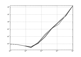
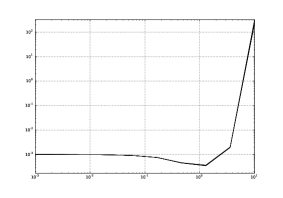
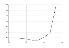
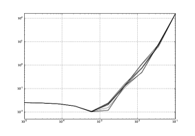
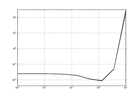
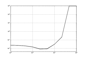
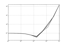
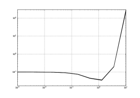
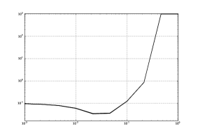
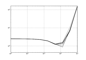
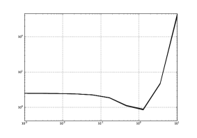
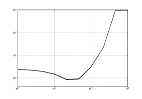
Figure 1: Prediction errors (y-axis) for experiment 1 (see text) for a varying $\lambda$ (x-axis) for procedure (4.1) (first column), procedure (4.2) (second column) and procedure (4.3) (third column). We plot the estimation errors over 10 simulated datasets (corresponding to a line in each figure), for an increasing noise level $\sigma=0.1$ (first line), $\sigma=0.5$ (second line), $\sigma=1.0$ (third line), $\sigma=5.0$ (fourth line). We can observe that the optimum $\lambda$ for (4.1) increases with $\sigma$ (see the position of minimum along the first column), while it can be kept almost constant for procedures (4.2) and (4.3)

Noise level $\sigma$	0.1	0.5	1.0	5.0
Procedure (4.1)	3.56e-04	1.03e-02	4.01e-02	1.17e+00
	(4.90e-05)	(2.23e-04)	(4.02e-03)	(1.52e-01)
Procedure (4.2)	3.54e-04	8.87e-03	3.54e-02	8.72e-01
	(8.66e-06)	(2.01e-04)	(8.34e-04)	(2.17e-02)
Procedure (4.3)	3.47e-04	8.65e-03	3.43e-02	8.54e-01
	(5.16e-06)	(1.44e-04)	(6.73e-04)	(1.56e-02)

Table 1: Average best prediction error (and standard deviation) for experiment 1 of the considered procedures for several values $\sigma$. Procedure (4.3) introduced in this paper always leads to a slight improvement.

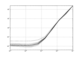
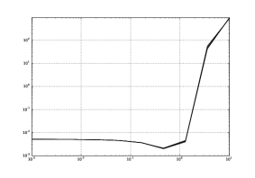
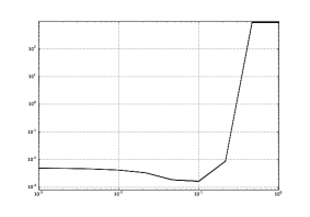
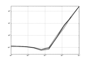
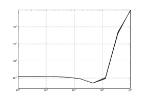
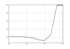
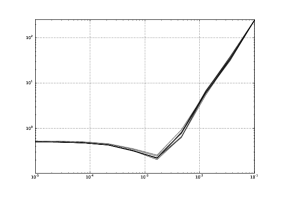
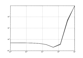
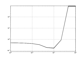
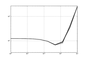
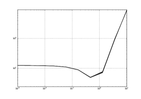
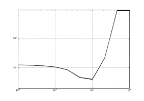
Figure 2: Prediction errors (y-axis) for experiment 2 (see text) for a varying $\lambda$ (x-axis) for procedure (4.1) (first column), procedure (4.2) (second column) and procedure (4.3) (third column). We plot the estimation errors over 10 simulated datasets (corresponding to a line in each figure), for an increasing noise level $\sigma=0.1$ (first line), $\sigma=0.5$ (second line), $\sigma=1.0$ (third line), $\sigma=5.0$ (fourth line). We can observe that the optimum $\lambda$ for (4.1) increases with $\sigma$ (see the position of minimum along the first column), while it can be kept almost constant for procedures (4.2) and (4.3)

Noise level $\sigma$	0.1	0.5	1.0	5.0
Procedure (4.1)	1.50e-02	6.37e-02	2.24e-01	6.87e+00
	(7.82e-03)	(5.59e-03)	(1.42e-02)	(1.17e-01)
Procedure (4.2)	2.05e-03	5.01e-02	2.01e-01	4.95e+00
	(5.37e-05)	(4.93e-04)	(1.79e-03)	(5.63e-02)
Procedure (4.3)	1.64e-03	4.10e-02	1.64e-01	3.93e+00
	(2.61e-05)	(4.40e-04)	(2.78e-03)	(5.87e-02)

Table 2: Average best prediction error (and standard deviation) for experiment 2 of the considered procedures for several values $\sigma$. Procedure (4.3) introduced in this paper leads to a strong improvement in this case.

Appendix A Proof of Theorem 1

The proof of Theorem 1 is based on the ideas of the proof of Theorem 1 in [18]. However, as the statistical structure of our estimator is different from that of the estimator proposed in [18], the proof requires several modifications and additional information on the behaviour of the estimator. This information is given in Lemmas 4 and 5. In particular, Lemma 4 provides a bound on the rank of our estimator. Its proof is given in Appendix B

Lemma 4.

$${\rm rank}(\hat{A})\leq 1/\lambda^{2}.$$

Lemma 5.

Suppose that $\dfrac{\rho}{\sqrt{{\rm rank}(A_{0})}}\geq\lambda\geq 3\Delta$ for some $\rho<1$, then

$$\|\hat{A}-\mathbf{X}\|_{2}\;\geq\left(\dfrac{3-\sqrt{1+\rho^{2}}}{3+\sqrt{1+\rho^{2}}}\right)\|A_{0}-\mathbf{X}\|_{2}$$ (A.1)

If $\hat{A}=\mathbf{X}$, then (A.1) implies that $A_{0}=\mathbf{X}$ and we get $\|\hat{A}-A_{0}\|_{2}=0$.
When $\hat{A}\neq\mathbf{X}$, we will use the fact that the subdifferential of the convex function $A\rightarrow\|A\|_{1}$ is the following set of matrices (cf. [27])

$$\partial\|A\|_{1}=\left\{\underset{j=1}{\overset{{\rm rank}(A)}{\sum}}u_{j}(A)v_{j}^{T}(A)+\mathcal{P}_{S_{1}^{\bot}(A)}W\mathcal{P}_{S_{2}^{\bot}(A)}\;:\;\|W\|_{\infty}\leq 1\right\}.$$ (A.2)

Here $u_{j}(A)$ and $v_{j}(A)$ are respectively the left and right orthonormal singular vectors of $A$, $S_{1}(A)$ is the linear span of $\{u_{j}(A)\}$, $S_{2}(A)$ is the linear span of $\{v_{j}(A)\}$. For simplicity we will write $u_{j}$ and $v_{j}$ instead of $u_{j}(A)$ and $v_{j}(A)$. A necessary condition of extremum in (2.6) implies that there exists $\hat{V}\in\partial\|\hat{A}\|_{1}$ such that for any $A\in\mathbb{R}^{m_{1}\times m_{2}}$

$$\begin{split}\dfrac{2\langle\hat{A}-\mathbf{X},\hat{A}-A\rangle}{2\|\hat{A}-\mathbf{X}\|_{2}}+\lambda\langle\hat{V},\hat{A}-A\rangle\leq 0.\end{split}$$ (A.3)

By the monotonicity of subdifferentials of convex functions we have that $\langle\hat{V}-V,\hat{A}-A\rangle\geq 0$ where $V\in\partial\|A\|_{1}$. Then (A.3) and $2\langle\hat{A}-A_{0},\hat{A}-A\rangle=\|\hat{A}-A_{0}\|^{2}_{2}+\|\hat{A}-A\|^{2}_{2}-\|A-A_{0}\|^{2}_{2}$ imply

$$\begin{split}&\|\hat{A}-A_{0}\|^{2}_{2}+\|\hat{A}-A\|^{2}_{2}+2\lambda\|\hat{A}-\mathbf{X}\|_{2}\left\langle\mathcal{P}_{S_{1}^{\bot}(A)}W\mathcal{P}_{S_{2}^{\bot}(A)},\hat{A}-A\right\rangle\\ &\hskip 14.22636pt\leq\|A-A_{0}\|^{2}_{2}+2\langle\mathbf{X}-A_{0},\hat{A}-A\rangle-2\lambda\|\hat{A}-\mathbf{X}\|_{2}\left\langle\underset{j=1}{\overset{r}{\sum}}u_{j}v_{j}^{T},\hat{A}-A\right\rangle.\end{split}$$ (A.4)

For $B$, a $m_{1}\times m_{2}$ matrix, let $\mathbf{Pr}_{A}(B)=B-\mathcal{P}_{S_{1}^{\bot}(A)}B\mathcal{P}_{S_{2}^{\bot}(A)}$. Since

$$\mathbf{Pr}_{A}(B)=\mathcal{P}_{S_{1}^{\bot}(A)}B\mathcal{P}_{S_{2}(A)}+\mathcal{P}_{S_{1}(A)}B$$

and ${\rm rank}(\mathcal{P}_{S_{i}(A)}B)\leq{\rm rank}(A)$ we have that ${\rm rank}(\mathbf{Pr}_{A}(B))\leq 2{\rm rank}(A)$.

Now, we consider each term in (A.4) separately. First, using the trace duality and triangle inequality, we get

$$\begin{split}\langle\mathbf{X}-A_{0},\hat{A}-A\rangle&\leq\|\mathbf{X}-A_{0}\|_{\infty}\|\hat{A}-A\|_{1}\\ &\leq\|\mathbf{X}-A_{0}\|_{\infty}\left\|\mathbf{Pr}_{A}\left(\hat{A}-A\right)\right\|_{1}\\ &\hskip 14.22636pt+\|\mathbf{X}-A_{0}\|_{\infty}\left\|\mathcal{P}_{S_{1}^{\bot}(A)}\left(\hat{A}-A\right)\mathcal{P}_{S_{2}^{\bot}(A)}\right\|_{1}.\end{split}$$ (A.5)

Note that $\left\|\underset{j=1}{\overset{r}{\sum}}u_{j}v_{j}^{T}\right\|_{\infty}=1$. Then, the trace duality implies

$$\left\langle\underset{j=1}{\overset{r}{\sum}}u_{j}v_{j}^{T},\hat{A}-A\right\rangle=\left\langle\underset{j=1}{\overset{r}{\sum}}u_{j}v_{j}^{T},\mathbf{Pr}_{A}\left(\hat{A}-A\right)\right\rangle\leq\left\|\mathbf{Pr}_{A}\left(\hat{A}-A\right)\right\|_{1}.$$ (A.6)

From the trace duality, we get that, there exists $W$ with $\|W\|_{\infty}\leq 1$ such that

$$\begin{split}\left\langle\mathcal{P}_{S_{1}^{\bot}(A)}W\mathcal{P}_{S_{2}^{\bot}(A)},\hat{A}-A\right\rangle&=\left\langle W,\mathcal{P}_{S_{1}^{\bot}(A)}\left(\hat{A}-A\right)\mathcal{P}_{S_{2}^{\bot}(A)}\right\rangle\\ &=\left\|\mathcal{P}_{S_{1}^{\bot}(A)}\left(\hat{A}-A\right)\mathcal{P}_{S_{2}^{\bot}(A)}\right\|_{1}.\end{split}$$ (A.7)

Using (A.1) and the definition of $\lambda$ we derive

$$\begin{split}\lambda\|\hat{A}-\mathbf{X}\|_{2}\left\|\mathcal{P}_{S_{1}^{\bot}(A)}\;\hat{A}\;\mathcal{P}_{S_{2}^{\bot}(A)}\right\|_{1}&\geq\lambda\dfrac{3-\sqrt{1+\rho^{2}}}{3+\sqrt{1+\rho^{2}}}\|A_{0}-\mathbf{X}\|_{2}\left\|\mathcal{P}_{S_{1}^{\bot}(A)}\;\hat{A}\;\mathcal{P}_{S_{2}^{\bot}(A)}\right\|_{1}\\ &\geq 3\dfrac{3-\sqrt{1+\rho^{2}}}{3+\sqrt{1+\rho^{2}}}\|A_{0}-\mathbf{X}\|_{\infty}\|\mathcal{P}_{S_{1}^{\bot}(A)}\;\hat{A}\;\mathcal{P}_{S_{2}^{\bot}(A)}\|_{1}.\end{split}$$ (A.8)

Note that $6\dfrac{3-\sqrt{1+\rho^{2}}}{3+\sqrt{1+\rho^{2}}}\geq 2$ for any $\rho<1$. Thus, putting (A.5), (A.6) and (A.8) into (A.4) yield

$$\begin{split}\|\hat{A}-A_{0}\|^{2}_{2}+\|\hat{A}-A\|^{2}_{2}&\leq\|A-A_{0}\|^{2}_{2}+2\|\mathbf{X}-A_{0}\|_{\infty}\|\mathbf{Pr}_{A}\left(\hat{A}-A\right)\|_{1}\\ &\hskip 14.22636pt+2\lambda\|\hat{A}-\mathbf{X}\|_{2}\|\mathbf{Pr}_{A}\left(\hat{A}-A\right)\|_{1}.\end{split}$$ (A.9)

Now, using the triangle inequality and the fact that

$$\left\|\mathbf{Pr}_{A}\left(\hat{A}-A\right)\right\|_{1}\leq\sqrt{2{\rm rank}(A)}\|\hat{A}-A\|_{2}$$

we get

$$\begin{split}&2\left\|\mathbf{X}-A_{0}\right\|_{\infty}\left\|\mathbf{Pr}_{A}\left(\hat{A}-A\right)\right\|_{1}+2\lambda\left\|\hat{A}-\mathbf{X}\right\|_{2}\left\|\mathbf{Pr}_{A}\left(\hat{A}-A\right)\right\|_{1}\\ &\hskip 14.22636pt\leq 2\Big{(}\left\|\mathbf{X}-A_{0}\right\|_{\infty}+\lambda\left\|\mathbf{X}-A_{0}\right\|_{2}\Big{)}\sqrt{2{\rm rank}(A)}\left\|\hat{A}-A\right\|_{2}\\ &\hskip 71.13188pt+2\lambda\|\hat{A}-A_{0}\|_{2}\sqrt{2{\rm rank}(A)}\|\hat{A}-A\|_{2}.\end{split}$$ (A.10)

From the definition of $\lambda$ we get that $\left\|\mathbf{X}-A_{0}\right\|_{\infty}\leq\lambda\left\|\mathbf{X}-A_{0}\right\|_{2}/3$. For $A$ such that $\lambda\sqrt{2{\rm rank}(A)}\leq\rho$, (A.10) implies

$$\begin{split}\|\hat{A}-A_{0}\|^{2}_{2}+\|\hat{A}-A\|^{2}_{2}&\leq\|A-A_{0}\|^{2}_{2}+\dfrac{8}{3}\lambda\|\mathbf{X}-A_{0}\|_{2}\sqrt{2{\rm rank}(A)}\|\hat{A}-A\|_{2}\\ &\hskip 28.45274pt+2\rho\|\hat{A}-A_{0}\|_{2}\|\hat{A}-A\|_{2}.\end{split}$$

Using $2ab\leq a^{2}+b^{2}$ twice we finally compute

$$\begin{split}(1-\rho)\|\hat{A}-A_{0}\|^{2}_{2}\leq\|A-A_{0}\|^{2}_{2}+\dfrac{4}{1-\rho}\lambda^{2}\|\mathbf{X}-A_{0}\|_{2}^{2}{\rm rank}(A)\end{split}$$

which implies the statement of Theorem 1.

Appendix B Proof of Lemma 4

That $\hat{A}$ is the minimum of (2.6) implies that $0\in\partial F(\hat{A})$. For $\hat{A}\neq\mathbf{X}$, (A.2) implies that there exists a matrix $W$ such that $\|W\|_{\infty}\leq 1$ and

$$\dfrac{\hat{A}-\mathbf{X}}{\|\hat{A}-\mathbf{X}\|_{2}}=-\lambda\underset{j=1}{\overset{{\rm rank}(\hat{A})}{\sum}}u_{j}(\hat{A})v_{j}^{T}(\hat{A})-\lambda\mathcal{P}_{S_{1}^{\bot}(\hat{A})}W\mathcal{P}_{S_{2}^{\bot}(\hat{A})}.$$ (B.1)

Calculating the $\|\cdot\|_{2}^{2}$ norm of both sides of (B.1) we get that $1\geq\lambda^{2}{\rm rank}(\hat{A})$.

When $\hat{A}=\mathbf{X}$, instead of the differential of $\|\hat{A}-\mathbf{X}\|_{2}$ we use its subdifferential: in (B.1) the term $\dfrac{\hat{A}-\mathbf{X}}{\|\hat{A}-\mathbf{X}\|_{2}}$ is replaced by a matrix $\tilde{W}$ such that $\|\tilde{W}\|_{2}\leq 1$ and we get again $1\geq\lambda^{2}{\rm rank}(\hat{A})$.

Appendix C Proof of Lemma 5

If $A_{0}=\mathbf{X}$, then, we have trivially $\|\hat{A}-\mathbf{X}\|_{2}\;\geq 0$.

If $A_{0}\neq\mathbf{X}$, by the convexity of the function $A\rightarrow\|A-\mathbf{X}\|_{2}$, we have

$$\begin{split}\|\hat{A}-\mathbf{X}\|_{2}-\|A_{0}-\mathbf{X}\|_{2}&\geq\dfrac{\langle A_{0}-\mathbf{X},\hat{A}-A_{0}\rangle}{\|A_{0}-\mathbf{X}\|_{2}}\\ &\geq-\dfrac{\|A_{0}-\mathbf{X}\|_{\infty}}{\|A_{0}-\mathbf{X}\|_{2}}\|\hat{A}-A_{0}\|_{1}\\ &\geq-\dfrac{\|A_{0}-\mathbf{X}\|_{\infty}}{\|A_{0}-\mathbf{X}\|_{2}}\sqrt{{\rm rank}(\hat{A})+{\rm rank}(A_{0})}\|\hat{A}-A_{0}\|_{2}.\end{split}$$ (C.1)

Using Lemma 4, the bound $\dfrac{\rho}{\sqrt{{\rm rank}(A_{0})}}\geq\lambda$ and the triangle inequality, from (C.1) we get

$$\begin{split}\|\hat{A}-\mathbf{X}\|_{2}-\|A_{0}-\mathbf{X}\|_{2}&\geq\\ &\hskip-14.22636pt-\dfrac{\sqrt{1+\rho^{2}}}{\lambda}\dfrac{\|A_{0}-\mathbf{X}\|_{\infty}}{\|A_{0}-\mathbf{X}\|_{2}}\left(\|\hat{A}-\mathbf{X}\|_{2}+\|A_{0}-\mathbf{X}\|_{2}\right).\end{split}$$ (C.2)

Note that $\dfrac{\|A_{0}-\mathbf{X}\|_{\infty}}{\lambda\|A_{0}-\mathbf{X}\|_{2}}\leq 1/3$ which finally leads to

$$\left(1+\dfrac{\sqrt{1+\rho^{2}}}{3}\right)\|\hat{A}-\mathbf{X}\|_{2}\;\geq\left(1-\dfrac{\sqrt{1+\rho^{2}}}{3}\right)\|A_{0}-\mathbf{X}\|_{2}.$$

This completes the proof of Lemma 5.

Appendix D Proof of Lemma 1

Our goal is to get a numerical estimation on $c_{*}$ in the case of Gaussian noise. Let $Z_{i}=\xi_{i}\left(X_{i}-\mathbb{E}X_{i}\right)$ and

$$\sigma_{Z}=\max\left\{\left\|\dfrac{1}{n}\overset{n}{\underset{i=1}{\sum}}\mathbb{E}\left(Z_{i}Z^{T}_{i}\right)\right\|^{1/2}_{\infty},\left\|\dfrac{1}{n}\overset{n}{\underset{i=1}{\sum}}\mathbb{E}\left(Z_{i}^{{}^{T}}Z_{i}\right)\right\|^{1/2}_{\infty}\right\}=\dfrac{1}{m_{1}\wedge m_{2}}.$$

The constant $c_{*}$ comes up in the proof of Lemma 2 in [18] in the estimation of

$$\Delta_{1}=\left\|\dfrac{1}{n}\overset{n}{\underset{i=1}{\sum}}\xi_{i}X_{i}\right\|_{\infty}\leq\left\|\dfrac{1}{n}\overset{n}{\underset{i=1}{\sum}}\xi_{i}\left(X_{i}-\mathbb{E}X_{i}\right)\right\|_{\infty}+\dfrac{1}{\sqrt{m_{1}m_{2}}}\left|\dfrac{1}{n}\overset{n}{\underset{i=1}{\sum}}\xi_{i}\right|.$$

A standard application of Markov’s inequality gives that, with probability at least $1-1/m$

$$\dfrac{1}{\sqrt{m_{1}m_{2}}}\left|\dfrac{1}{n}\overset{n}{\underset{i=1}{\sum}}\xi_{i}\right|\leq 2\sqrt{\dfrac{\log m}{nm_{1}m_{2}}}.$$ (D.1)

In [18], the authors estimate $\left\|\dfrac{1}{n}\overset{n}{\underset{i=1}{\sum}}\xi_{i}\left(X_{i}-\mathbb{E}X_{i}\right)\right\|_{\infty}$ using [17, Proposition 2]. To get a numerical estimation on $c_{*}$ we follow the lines of the proof of [17, Proposition 2]. In order to simplify notations, we write $\|\;\|_{\infty}=\|\;\|$ and we consider the case of Hermitian matrices of size $m^{\prime}$. Its extension to rectangular matrices is straightforward via self-adjoint dilation, cf., for example, 2.6 in [25].

Let $Y_{n}=\overset{n}{\underset{i=1}{\sum}}Z_{i}$. In the proof of [17, Proposition 2], after following the standard derivation of the classical Bernstein inequality and using the Golden-Thompson inequality, the author derives the following bound

$$\mathbb{P}\left(\|Y_{n}\|\geq t\right)\leq 2m^{\prime}e^{-\lambda t}\|\mathbb{E}e^{\lambda Z_{1}}\|^{n}$$ (D.2)

and

$$\|\mathbb{E}e^{\lambda Z_{1}}\|\leq 1+\lambda^{2}\left\|\mathbb{E}Z_{1}^{2}\left[\dfrac{e^{\lambda\|Z_{1}\|}-1-\lambda\|Z_{1}\|}{\lambda^{2}\|Z_{1}\|^{2}}\right]\right\|.$$ (D.3)

Using that $\|Z_{1}\|\leq 2|\xi_{i}|$, from (D.3), we compute

$$\begin{split}\left\|\mathbb{E}e^{\lambda Z_{1}}\right\|&\leq 1+\lambda^{2}\left\|\mathbb{E}\left[\left(X_{i}-\mathbb{E}X_{i}\right)^{2}\right]\mathbb{E}\left(\xi_{i}^{2}\left[\dfrac{e^{2\lambda|\xi_{i}|}-1-2\lambda|\xi_{i}|}{4\lambda^{2}\xi_{i}^{2}}\right]\right)\right\|\\ &\hskip 14.22636pt\leq 1+\lambda^{2}\sigma_{Z}^{2}\mathbb{E}\left(\dfrac{(2|\xi_{i}|)^{2}}{2!}+\dfrac{\lambda(2|\xi_{i}|)^{3}}{3!}+\cdots\right).\end{split}$$ (D.4)

Assume that $\lambda<1$, then (D.4) implies

$$\begin{split}\left\|\mathbb{E}e^{\lambda Z_{1}}\right\|\leq 1+\lambda^{2}\sigma_{Z}^{2}\mathbb{E}e^{2|\xi_{i}|}\leq 1+2\lambda^{2}\sigma_{Z}^{2}e^{2}\leq\exp\{2\lambda^{2}\sigma_{Z}^{2}e^{2}\}.\end{split}$$

Using this bound, from (D.2) we get

$$\mathbb{P}\left(\|Y_{n}\|\geq t\right)\leq 2m^{\prime}\exp\{-\lambda t+2\lambda^{2}\sigma_{Z}^{2}e^{2}\}.$$

It remains now to minimize the last bound with respect to $\lambda\in(0,1)$ to obtain that

$$\mathbb{P}\left(\|Y_{n}\|\geq t\right)\leq 2m^{\prime}\exp\left\{-\dfrac{t^{2}}{4e^{2}\sigma_{Z}^{2}n}\right\}$$

where we supposed that $n$ is large enough.

Putting $2m^{\prime}\exp\left\{-\dfrac{t^{2}}{4\sigma_{Z}^{2}e^{2}n}\right\}=1/(2m^{\prime})$, we get $t=2e\sqrt{\dfrac{2\log(2m^{\prime})n}{m_{1}\wedge m_{2}}}$. Using (D.1) we compute the following bound on $c_{*}$

$$c_{*}\leq 2e+1\leq 6.5.$$

This completes the proof of Lemma 1.

Appendix E Proof of Lemma 2

Let $\epsilon_{i}=\sigma\xi_{i}$. To prove (i) we compute

$$\begin{split}\left\langle\mathbf{M},\mathbf{M}\right\rangle&=\dfrac{\left\|A_{0}\right\|_{2}^{2}}{\left(m_{1}m_{2}\right)^{2}}+\left(1-\dfrac{2n}{m_{1}m_{2}}\right)\underset{\mathbf{I}}{\underbrace{\dfrac{1}{n^{2}}\overset{n}{\underset{i=1}{\sum}}\left\langle A_{0},X_{i}\right\rangle^{2}}}+\underset{\mathbf{II}}{\underbrace{\dfrac{1}{n^{2}}\overset{n}{\underset{i=1}{\sum}}\epsilon_{i}^{2}}}\\ &\hskip 14.22636pt+\left(1-\dfrac{n}{m_{1}m_{2}}\right)\underset{\mathbf{III}}{\underbrace{\dfrac{2}{n^{2}}\overset{n}{\underset{i=1}{\sum}}\left\langle A_{0},X_{i}\right\rangle\epsilon_{i}}}+\underset{\mathbf{IV}}{\underbrace{\dfrac{4}{n^{2}}\underset{i<j}{\sum}\epsilon_{i}\left\langle A_{0},X_{j}\right\rangle\left\langle X_{i},X_{j}\right\rangle}}\\ &\hskip 28.45274pt+\underset{\mathbf{V}}{\underbrace{\dfrac{2}{n^{2}}\underset{i<j}{\sum}\epsilon_{i}\epsilon_{j}\left\langle X_{i},X_{j}\right\rangle}}+\underset{\mathbf{VI}}{\underbrace{\dfrac{1}{n^{2}}\underset{i\neq j}{\sum}\left\langle A_{0},X_{i}\right\rangle\left\langle A_{0},X_{j}\right\rangle\left\langle X_{j},X_{i}\right\rangle}}.\end{split}$$ (E.1)

We estimate each term in (E.1) separately with a good probability.

• We have that $\mathbb{E}\left(\dfrac{1}{n^{2}}\overset{n}{\underset{i=1}{\sum}}\left\langle A_{0},X_{i}\right\rangle^{2}\right)=\dfrac{\left\|A_{0}\right\|^{2}_{2}}{nm_{1}m_{2}}$ and $\left|\left\langle A_{0},X_{i}\right\rangle\right|\leq a$.
  Using Hoeffding’s inequality , we get that, with probability at least
  $1-2\exp\left\{-2\sigma^{4}n/(8a)^{2}\right\}$

  $$\dfrac{\left\|A_{0}\right\|^{2}_{2}}{nm_{1}m_{2}}+\dfrac{\sigma^{2}}{8\,n}\geq\dfrac{1}{n^{2}}\overset{n}{\underset{i=1}{\sum}}\left\langle A_{0},X_{i}\right\rangle^{2}\geq\dfrac{\left\|A_{0}\right\|^{2}_{2}}{nm_{1}m_{2}}-\dfrac{\sigma^{2}}{8\,n}.$$

• $\epsilon_{i}^{2}$ are sub-exponential random variables and $\mathbb{E}\left(\dfrac{1}{n^{2}}\overset{n}{\underset{i=1}{\sum}}\epsilon_{i}^{2}\right)=\dfrac{\sigma^{2}}{n}$. Using Bernstein inequality for sub-exponentials random variables (cf. [26, Proposition 16] ) we get that, with probability at least
  $1-2\exp\left\{-cn\min\left[\sigma^{2}K/8^{2},\sigma\sqrt{K}/8\right]\right\}$

  $$\dfrac{\sigma^{2}}{n}+\dfrac{\sigma^{2}}{8n}\geq\dfrac{1}{n^{2}}\overset{n}{\underset{i=1}{\sum}}\epsilon_{i}^{2}\geq\dfrac{\sigma^{2}}{n}-\dfrac{\sigma^{2}}{8n}.$$

• We have that $\mathbb{E}\left(\dfrac{2}{n^{2}}\overset{n}{\underset{i=1}{\sum}}\left\langle A_{0},X_{i}\right\rangle\epsilon_{i}\right)=0$, using Hoeffding’s type inequality for sub-Gaussian random variables (cf. [26, Proposition 10]) we get that, with probability at least $1-e\exp\left\{-c\sigma^{2}Kn/a^{2}\right\}$

  $$\dfrac{\sigma^{2}}{8n}\geq\dfrac{2}{n^{2}}\overset{n}{\underset{i=1}{\sum}}\left\langle A_{0},X_{i}\right\rangle\epsilon_{i}\geq-\dfrac{\sigma^{2}}{8n}.$$

• We compute $\mathbb{E}\left(\dfrac{4}{n^{2}}\underset{i<j}{\sum}\epsilon_{i}\left\langle A_{0},X_{j}\right\rangle\left\langle X_{i},X_{j}\right\rangle\right)=0$. We use the following lemma which is proven in the Appendix F.

  Lemma 6.

  Suppose that $n\leq m_{1}m_{2}$. With probability at least
  $1-\dfrac{2}{m_{1}m_{2}}$

  $$\underset{i<j}{\sum}\left\langle X_{i},X_{j}\right\rangle\leq n.$$

  Lemma 6 and Hoeffding’s type inequality imply that, with probability at least $1-2/m_{1}m_{2}-e\exp\left\{-c\sigma^{2}nK/a^{2}\right\}$

  $$\dfrac{\sigma^{2}}{8n}\geq\dfrac{4}{n^{2}}\underset{i<j}{\sum}\epsilon_{i}\left\langle A_{0},X_{j}\right\rangle\left\langle X_{i},X_{j}\right\rangle\geq-\dfrac{\sigma^{2}}{8n}$$

• We have that $\mathbb{E}\left(\dfrac{2}{n^{2}}\underset{i<j}{\sum}\epsilon_{i}\epsilon_{j}\left\langle X_{i},X_{j}\right\rangle\right)=0$. Using Bernstein inequality for sub-exponentials random variables (cf. [26, Proposition 16] ) and Lemma 6 we get that, with probability at least $1-2\exp\left\{-cn\min\left[\sigma^{2}K/8^{2},\sigma\sqrt{K}/8\right]\right\}$

  $$\dfrac{\sigma^{2}}{8n}\geq\dfrac{2}{n^{2}}\underset{i<j}{\sum}\epsilon_{i}\epsilon_{j}\left\langle X_{i},X_{j}\right\rangle\geq-\dfrac{\sigma^{2}}{8n}.$$

• We compute that

  $$\begin{split}\mathbb{E}\left(\dfrac{1}{n^{2}}\underset{i\neq j}{\sum}\left\langle A_{0},X_{i}\right\rangle\left\langle A_{0},X_{j}\right\rangle\left\langle X_{j},X_{i}\right\rangle\right)&=\dfrac{1}{n^{2}}\underset{i\neq j}{\sum}\left\langle\mathbb{E}\left(\left\langle A_{0},X_{j}\right\rangle X_{j}\right),\mathbb{E}\left(\left\langle A_{0},X_{i}\right\rangle X_{i}\right)\right\rangle\\ &=\dfrac{1}{n^{2}}\underset{i\neq j}{\sum}\dfrac{\left\|A_{0}\right\|^{2}_{2}}{\left(m_{1}m_{2}\right)^{2}}\\ &\leq\dfrac{\left\|A_{0}\right\|^{2}_{2}}{\left(m_{1}m_{2}\right)^{2}}.\end{split}$$

  Using Lemma 6 and Hoeffding’s type inequality for sub-Gaussian random variables (cf. [26, Proposition 10]), we get that, with probability at least $1-2/m_{1}m_{2}-2\exp\left\{-2\sigma^{4}n/(8a)^{2}\right\}$

  $$\dfrac{1}{n^{2}}\underset{i\neq j}{\sum}\left\langle A_{0},X_{i}\right\rangle\left\langle A_{0},X_{j}\right\rangle\left\langle X_{j},X_{i}\right\rangle\leq\dfrac{\left\|A_{0}\right\|^{2}_{2}}{(m_{1}m_{2})^{2}}+\dfrac{\sigma^{2}}{8n}.$$

To obtain the lower bound, note that, for $i\neq j$, $\left\langle X_{i},X_{j}\right\rangle\neq 0$ iff $X_{i}=X_{j}$. This implies that $\underset{i\neq j}{\sum}\left\langle A_{0},X_{i}\right\rangle\left\langle A_{0},X_{j}\right\rangle\left\langle X_{j},X_{i}\right\rangle\geq 0$. We use that $2n<m_{1}m_{2}$ to get

$$\dfrac{\left\|A_{0}\right\|_{2}^{2}}{\left(m_{1}m_{2}\right)^{2}}+\left(1-\dfrac{2n}{m_{1}m_{2}}\right)\dfrac{1}{n^{2}}\overset{n}{\underset{i=1}{\sum}}\left\langle A_{0},X_{i}\right\rangle^{2}\geq 0.$$

Putting the lower bounds in $\mathbf{II}-\mathbf{V}$ together we compute from (E.1)

$$\left\|\mathbf{M}\right\|^{2}_{2}\geq\dfrac{\sigma^{2}}{2\,n}.$$

To obtain the upper bound, we use the upper bounds in $\mathbf{I}-\mathbf{VI}$. From (E.1) we get

$$\left\|\mathbf{M}\right\|^{2}_{2}\leq\dfrac{2\left\|A_{0}\right\|^{2}_{2}}{\left(m_{1}m_{2}\right)^{2}}+\dfrac{\left\|A_{0}\right\|^{2}_{2}}{nm_{1}m_{2}}+\dfrac{14\sigma^{2}}{8\,n}\leq 2\left(\dfrac{\left\|A_{0}\right\|^{2}_{2}}{nm_{1}m_{2}}+\dfrac{\sigma^{2}}{\,n}\right)$$

where we used that $2n\leq m_{1}m_{2}$. This completes the proof of part (i) in Lemma 2.

To prove (ii) we use that $\left\langle X_{i},X_{i}\right\rangle=1$ and $\left\langle X_{i},X_{j}\right\rangle\neq 0$ iff $X_{i}=X_{j}$. We compute

$$\begin{split}\dfrac{1}{n^{2}}\left\langle\overset{n}{\underset{i=1}{\sum}}Y_{i}X_{i},\overset{n}{\underset{i=1}{\sum}}Y_{i}X_{i}\right\rangle&=\dfrac{1}{n^{2}}\overset{n}{\underset{i=1}{\sum}}Y_{i}^{2}+\dfrac{2}{n^{2}}\underset{i<j}{\sum}Y_{i}Y_{j}\left\langle X_{i},X_{j}\right\rangle\\ &=\dfrac{1}{n^{2}}\overset{n}{\underset{i=1}{\sum}}\left(\left\langle A_{0},X_{i}\right\rangle^{2}+\epsilon_{i}^{2}+2\left\langle A_{0},X_{i}\right\rangle\epsilon_{i}\right)\\ &\hskip 14.22636pt+\dfrac{2}{n^{2}}\underset{i<j}{\sum}\left\langle A_{0},X_{i}\right\rangle^{2}\left\langle X_{i},X_{j}\right\rangle\\ &\hskip 21.33955pt+\dfrac{4}{n^{2}}\underset{i<j}{\sum}\epsilon_{i}\left\langle A_{0},X_{j}\right\rangle\left\langle X_{i},X_{j}\right\rangle+\dfrac{2}{n^{2}}\underset{i<j}{\sum}\epsilon_{i}\epsilon_{j}\left\langle X_{i},X_{j}\right\rangle.\end{split}$$

This implies that

$$\begin{split}\dfrac{1}{n^{2}}\left\langle\overset{n}{\underset{i=1}{\sum}}Y_{i}X_{i},\overset{n}{\underset{i=1}{\sum}}Y_{i}X_{i}\right\rangle&\geq\underset{\mathbf{I}}{\underbrace{\dfrac{1}{n^{2}}\overset{n}{\underset{i=1}{\sum}}\left\langle A_{0},X_{i}\right\rangle^{2}}}+\underset{\mathbf{II}}{\underbrace{\dfrac{1}{n^{2}}\overset{n}{\underset{i=1}{\sum}}\epsilon_{i}^{2}}}+\underset{\mathbf{III}}{\underbrace{\dfrac{2}{n^{2}}\overset{n}{\underset{i=1}{\sum}}\left\langle A_{0},X_{i}\right\rangle\epsilon_{i}}}\\ &\hskip 14.22636pt+\underset{\mathbf{IV}}{\underbrace{\dfrac{4}{n^{2}}\underset{i<j}{\sum}\epsilon_{i}\left\langle A_{0},X_{j}\right\rangle\left\langle X_{i},X_{j}\right\rangle}}+\underset{\mathbf{V}}{\underbrace{\dfrac{2}{n^{2}}\underset{i<j}{\sum}\epsilon_{i}\epsilon_{j}\left\langle X_{i},X_{j}\right\rangle}}.\end{split}$$ (E.2)

Using the lower bounds for $\mathbf{I}-\mathbf{V}$ we get from (E.2)

$$\dfrac{1}{n^{2}}\left\langle\overset{n}{\underset{i=1}{\sum}}Y_{i}X_{i},\overset{n}{\underset{i=1}{\sum}}Y_{i}X_{i}\right\rangle\geq\dfrac{\left\|A_{0}\right\|_{2}^{2}}{\,nm_{1}m_{2}}$$

which proves the part (ii) of Lemma 2.

(iii) is a consequence of (ii). For $4n\leq m_{1}m_{2}$ (ii) implies

$$\dfrac{1}{4n^{2}}\left\langle\overset{n}{\underset{i=1}{\sum}}Y_{i}X_{i},\overset{n}{\underset{i=1}{\sum}}Y_{i}X_{i}\right\rangle\geq\dfrac{\left\|A_{0}\right\|_{2}^{2}}{\left(m_{1}m_{2}\right)^{2}}.$$

Now we complete the proof of part (iii) of Lemma 2 using that

$$\left\|\mathbf{M}\right\|_{2}\geq\left\|\dfrac{1}{n}\overset{n}{\underset{i=1}{\sum}}Y_{i}X_{i}\right\|_{2}-\dfrac{\left\|A_{0}\right\|_{2}}{m_{1}m_{2}}.$$

Appendix F Proof of Lemma 6

Recall that for $i\neq j$, $X_{i}$ and $X_{j}$ are independent. We compute the expectation

$$\mathbb{E}\left(\underset{i<j}{\sum}\left\langle X_{i},X_{j}\right\rangle\right)=\underset{i<j}{\sum}\left\langle\mathbb{E}X_{i},\mathbb{E}X_{j}\right\rangle=\dfrac{n(n-1)}{2m_{1}m_{2}}$$

and the variance

$$\begin{split}\mathbb{E}\left(\left(\underset{i<j}{\sum}\left\langle X_{i},X_{j}\right\rangle\right)^{2}\right)-\left(\mathbb{E}\left(\underset{i<j}{\sum}\left\langle X_{i},X_{j}\right\rangle\right)\right)^{2}&\\ &\hskip-170.71652pt=\mathbb{E}\left(\underset{\underset{i^{\prime}<j^{\prime}}{i<j}}{\sum}\left\langle X_{i},X_{j}\right\rangle\left\langle X_{i^{\prime}},X_{j^{\prime}}\right\rangle\right)-\underset{\underset{i^{\prime}<j^{\prime}}{i<j}}{\sum}\mathbb{E}\left(\left\langle X_{i},X_{j}\right\rangle\right)\mathbb{E}\left(\left\langle X_{i^{\prime}},X_{j^{\prime}}\right\rangle\right).\end{split}$$

When $i,j,i^{\prime},j^{\prime}$ are all distinct, $\mathbb{E}\left(\left\langle X_{i},X_{j}\right\rangle\left\langle X_{i^{\prime}},X_{j^{\prime}}\right\rangle\right)$ is cancelled by the corresponding term in $\underset{\underset{i^{\prime}<j^{\prime}}{i<j}}{\sum}\mathbb{E}\left(\left\langle X_{i},X_{j}\right\rangle\right)\mathbb{E}\left(\left\langle X_{i^{\prime}},X_{j^{\prime}}\right\rangle\right)$.

It remains to consider the following five cases: (1) $i=i^{\prime}$ and $j=j^{\prime}$; (2) $i=i^{\prime}$ and $j\neq j^{\prime}$; (3) $i\neq i^{\prime}$ and $j=j^{\prime}$; (4) $i=j^{\prime}$ and $j\neq i^{\prime}$; (5) $i^{\prime}=j$ and $j^{\prime}\neq i$.

Case (1): note that $\left\langle X_{i},X_{j}\right\rangle$ takes only two values $0$ or $1$, which implies that

$$\mathbb{E}\left(\left\langle X_{i},X_{j}\right\rangle^{2}\right)=\mathbb{E}\left(\left\langle X_{i},X_{j}\right\rangle\right)=\dfrac{1}{m_{1}m_{2}}.$$

Cases (2)-(5): in these four cases, we need to calculate $\mathbb{E}\left(\left\langle X_{i},X_{k}\right\rangle\left\langle X_{k},X_{j}\right\rangle\right)$ for $i\neq j$ and $k\notin\{i,j\}$. Note that $\mathcal{P}_{X_{k}}=\left\langle\,\cdot\,,X_{k}\right\rangle X_{k}$ is the orthogonal projector on the vector space spanned by $X_{k}$. We compute

$$\mathbb{E}\mathcal{P}_{X_{k}}=\dfrac{1}{m_{1}m_{2}}\mathrm{Id}$$

where $\mathrm{Id}$ is the identity application on $\mathbb{R}^{m_{1}\times m_{2}}$. Then, we get

$$\begin{split}\mathbb{E}\left(\left\langle\left\langle X_{i},X_{k}\right\rangle X_{k},X_{j}\right\rangle\right)&=\mathbb{E}\left(\left\langle\mathcal{P}_{X_{k}}\left(X_{i}\right),X_{j}\right\rangle\right)\\ &=\left\langle\mathbb{E}\left(\mathcal{P}_{X_{k}}\right)\left(\mathbb{E}X_{i}\right),\mathbb{E}X_{j}\right\rangle\\ &=\dfrac{1}{m_{1}m_{2}}\left\langle\mathbb{E}X_{i},\mathbb{E}X_{j}\right\rangle\\ &=\dfrac{1}{\left(m_{1}m_{2}\right)^{2}}.\end{split}$$

These terms are cancelled by the corresponding terms in $\underset{\underset{i^{\prime}<j^{\prime}}{i<j}}{\sum}\mathbb{E}\left(\left\langle X_{i},X_{j}\right\rangle\right)\mathbb{E}\left(\left\langle X_{i^{\prime}},X_{j^{\prime}}\right\rangle\right)$ as

$$\mathbb{E}\left(\left\langle X_{i},X_{k}\right\rangle\right)\mathbb{E}\left(\left\langle X_{k},X_{j}\right\rangle\right)=\dfrac{1}{(m_{1}m_{2})^{2}}.$$

Finally we get that

$$\mathbb{E}\left(\left(\underset{i<j}{\sum}\left\langle X_{i},X_{j}\right\rangle\right)^{2}\right)-\left(\mathbb{E}\left(\underset{i<j}{\sum}\left\langle X_{i},X_{j}\right\rangle\right)\right)^{2}\leq\dfrac{n(n-1)}{2m_{1}m_{2}}.$$

The Bienaymé-Tchebychev inequality implies that

$$\mathbb{P}\left(\underset{i<j}{\sum}\left\langle X_{i},X_{j}\right\rangle\geq n\right)\leq\dfrac{n(n-1)}{2m_{1}m_{2}\left(n-\dfrac{n(n-1)}{2m_{1}m_{2}}\right)^{2}}\leq\dfrac{2}{m_{1}m_{2}}$$

when $m_{1}m_{2}\geq n$. This completes the proof of Lemma 6.

Appendix G Proof of Theorem 3

The following lemma is the counterpart of Lemma 4 in the present setting. It is proven in the Appendix H.

Lemma 7.

$${\rm rank}(V\hat{A})\leq 1/\lambda^{2}.$$

We need the following auxiliary result, which corresponds to Lemma 5, and which is proven in the Appendix I.

Lemma 8.

Suppose that $\dfrac{\rho}{\sqrt{{\rm rank}(VA_{0})}}\geq\lambda\geq 3\Delta^{\prime}$ for some $\rho<1$, then

$$\left\|V\hat{A}-U\right\|_{2}\;\geq\left(\dfrac{3-\sqrt{1+\rho^{2}}}{3+\sqrt{1+\rho^{2}}}\right)\|E\|_{2}.$$

Now the proof of Theorem 3 is very similar to the proof of the Theorem 1. We only sketch it. If $V\hat{A}\neq U$, a necessary condition of extremum in (3) implies that there exists a $\hat{W}\in\partial\|V\hat{A}\|_{1}$ such that for any $A\in\mathbb{R}^{m_{1}\times m_{2}}$

$$\begin{split}\dfrac{2\left\langle V\hat{A}-U,V\left(\hat{A}-A\right)\right\rangle}{2\left\|V\hat{A}-U\right\|_{2}}+\lambda\left\langle\hat{W},V\left(\hat{A}-A\right)\right\rangle\leq 0.\end{split}$$ (G.1)

and we get

$$\begin{split}\left\|V\left(\hat{A}-A_{0}\right)\right\|^{2}_{2}+\left\|V\left(\hat{A}-A\right)\right\|^{2}_{2}+2\lambda\Big{\|}V\hat{A}-U\Big{\|}_{2}\left\langle\mathcal{P}_{S_{1}^{\bot}(VA)}W\mathcal{P}_{S_{2}^{\bot}(VA)},V\left(\hat{A}-A\right)\right\rangle&\\ &\hskip-341.43306pt\leq\big{\|}V\left(A-A_{0}\right)\big{\|}^{2}_{2}+2\left\langle E,V\left(\hat{A}-A\right)\right\rangle\\ &\hskip-256.0748pt-2\lambda\left\|V\hat{A}-U\right\|_{2}\left\langle\underset{j=1}{\overset{{\rm rank}(VA)}{\sum}}u_{j}(VA)v_{j}(VA)^{T},V\left(\hat{A}-A\right)\right\rangle.\end{split}$$ (G.2)

Let $\mathbf{Pr}_{VA}(B)=B-\mathcal{P}_{S_{1}^{\bot}(VA)}B\mathcal{P}_{S_{2}^{\bot}(VA)}$. Then, the trace duality and the triangle inequality imply

$$\begin{split}\left\langle E,V\left(\hat{A}-A\right)\right\rangle&=\left\langle\mathcal{P}_{V}E,V\left(\hat{A}-A\right)\right\rangle\\ &\leq\left\|\mathcal{P}_{V}E\right\|_{\infty}\left\|V\left(\hat{A}-A\right)\right\|_{1}\\ &\leq\left\|\mathcal{P}_{V}E\right\|_{\infty}\left\|\mathbf{Pr}_{VA}\left[V\left(\hat{A}-A\right)\right]\right\|_{1}\\ &\hskip 14.22636pt+\left\|\mathcal{P}_{V}E\right\|_{\infty}\left\|\mathcal{P}_{S_{1}^{\bot}(VA)}V\left(\hat{A}-A\right)\mathcal{P}_{S_{2}^{\bot}(VA)}\right\|_{1}.\end{split}$$ (G.3)

Using $6\dfrac{3-\sqrt{1+\rho^{2}}}{3+\sqrt{1+\rho^{2}}}\geq 2$ for any $\rho<1$ (G.2) implies

$$\begin{split}\left\|V\left(\hat{A}-A_{0}\right)\right\|^{2}_{2}+\left\|V\left(\hat{A}-A\right)\right\|^{2}_{2}&\leq\big{\|}V\left(A-A_{0}\right)\big{\|}^{2}_{2}\\ &\hskip 14.22636pt+2\left\|\mathcal{P}_{V}E\right\|_{\infty}\left\|\mathbf{Pr}_{VA}\left[V\left(\hat{A}-A\right)\right]\right\|_{1}\\ &\hskip 28.45274pt+2\lambda\left\|V\hat{A}-U\right\|_{2}\left\|\mathbf{Pr}_{VA}\left[V\left(\hat{A}-A\right)\right]\right\|_{1}.\end{split}$$ (G.4)

Now we use $\left\|\mathbf{Pr}_{VA}\left[V\left(\hat{A}-A\right)\right]\right\|_{1}\leq\sqrt{2{\rm rank}(VA)}\left\|V\left(\hat{A}-A\right)\right\|_{2}$, $\left\|\mathcal{P}_{V}E\right\|_{\infty}\leq\lambda\|E\|_{2}/3$ and $\lambda\sqrt{2\,{\rm rank}(VA)}\leq\rho$ to conclude

$$\begin{split}(1-\rho)\left\|V\left(\hat{A}-A_{0}\right)\right\|^{2}_{2}\leq\big{\|}V\left(A-A_{0}\right)\big{\|}^{2}_{2}+\dfrac{4\lambda^{2}}{1-\rho}\|E\|_{2}^{2}\,{\rm rank}(VA)\end{split}$$

which implies the statement of Theorem 3.

Appendix H Proof of Lemma 7

That $\hat{A}$ is the minimum of (3) implies that $0\in\partial G(\hat{A})$ where

$$G=\|U-V\,A\|_{2}+\lambda\|VA\|_{1}.$$

Note that the subdifferential of the convex function $A\rightarrow\|VA\|_{1}$ is the following set of matrices

$$\partial\|VA\|_{1}=V^{T}\left\{\underset{j=1}{\overset{{\rm rank}(VA)}{\sum}}u_{j}(VA)v_{j}^{T}(VA)+\mathcal{P}_{S_{1}^{\bot}(VA)}W\mathcal{P}_{S_{2}^{\bot}(VA)}\;:\;\|W\|_{\infty}\leq 1\right\}$$

where $S_{1}(VA)$ is the linear span of $\{u_{j}(VA)\}$ and $S_{2}(VA)$ is the linear span of $\{v_{j}(VA)\}$.

If $\hat{A}$ is such that $V\hat{A}\neq U$, we obtain that, there exists a matrix $W$ such that $\|W\|_{\infty}\leq 1$ and

$$V^{T}\dfrac{V\hat{A}-U}{\|V\hat{A}-U\|_{2}}=-\lambda V^{T}\left\{\underset{j=1}{\overset{{\rm rank}(VA)}{\sum}}u_{j}(VA)v_{j}^{T}(VA)+\mathcal{P}_{S_{1}^{\bot}(VA)}W\mathcal{P}_{S_{2}^{\bot}(VA)}\right\}$$

which implies

$$V^{T}\mathcal{P}_{V}\dfrac{V\hat{A}-U}{\|V\hat{A}-U\|_{2}}=-\lambda V^{T}\mathcal{P}_{V}\left\{\underset{j=1}{\overset{{\rm rank}(VA)}{\sum}}u_{j}(VA)v_{j}^{T}(VA)+\mathcal{P}_{S_{1}^{\bot}(VA)}W\mathcal{P}_{S_{2}^{\bot}(VA)}\right\}.$$ (H.1)

Using $\mathcal{P}_{V}VA\left(v_{j}(VA)\right)=VA\left(v_{j}(VA)\right)=\sigma_{j}(VA)u_{j}(VA)$ and $\sigma_{j}\neq 0$ we get

$$\mathcal{P}_{V}u_{j}(VA)=u_{j}(VA).$$ (H.2)

Note that for any $w$ such that $\left\langle w,u_{j}(VA)\right\rangle=0$ (H.2) implies that

$$\left\langle\mathcal{P}_{V}w,u_{j}(VA)\right\rangle=\left\langle w,u_{j}(VA)\right\rangle=0.$$ (H.3)

By the definition, $\mathcal{P}_{S_{1}^{\bot}(VA)}$ projects on the orthogonal complement of the linear span of $\{u_{j}(VA)\}$. Thus, (H.3) implies that $\mathcal{P}_{V}\mathcal{P}_{S_{1}^{\bot}(VA)}$ also projects on the subspace orthogonal to the linear span of $\{u_{j}(VA)\}$.

Note that $V^{T}\mathcal{P}_{V}B=0$ imply $\mathcal{P}_{V}B=0$ and we get from (H.1)

$$\mathcal{P}_{V}\dfrac{V\hat{A}-U}{\|V\hat{A}-U\|_{2}}=-\lambda\left\{\underset{j=1}{\overset{{\rm rank}(VA)}{\sum}}u_{j}(VA)v_{j}^{T}(VA)+\mathcal{P}_{V}\left[\mathcal{P}_{S_{1}^{\bot}(VA)}W\mathcal{P}_{S_{2}^{\bot}(VA)}\right]\right\}.$$ (H.4)

Calculating the $\|\;\|_{2}^{2}$ norm of both sides of (H.4) we get that $1\geq\lambda^{2}{\rm rank}(V\hat{A})$. When $V\hat{A}=U$, instead of the differential of $\|U-V\,A\|_{2}$ we use its subdiffential.

Appendix I Proof of Lemma 8

If $VA_{0}=U$, then we have trivially $\|V\hat{A}-U\|_{2}\;\geq 0.$ If $VA_{0}\neq U$, by the convexity of function $A\rightarrow\|VA-U\|_{2}$, we have

$$\begin{split}\left\|V\hat{A}-U\right\|_{2}-\left\|VA_{0}-U\right\|_{2}&\geq\dfrac{\left\langle VA_{0}-U,V\left(\hat{A}-A_{0}\right)\right\rangle}{\left\|VA_{0}-U\right\|_{2}}\\ &=\dfrac{\left\langle\mathcal{P}_{V}\left(E\right),V\left(\hat{A}-A_{0}\right)\right\rangle}{\left\|VA_{0}-U\right\|_{2}}\\ &\geq-\dfrac{\left\|\mathcal{P}_{V}\left(E\right)\right\|_{\infty}}{\left\|E\right\|_{2}}\left\|V\left(\hat{A}-A_{0}\right)\right\|_{1}\\ &\geq-\dfrac{\left\|\mathcal{P}_{V}\left(E\right)\right\|_{\infty}}{\left\|E\right\|_{2}}\sqrt{{\rm rank}(VA_{0})+{\rm rank}(V\hat{A})}\left\|V\left(\hat{A}-A_{0}\right)\right\|_{2}.\end{split}$$ (I.1)

Using the bound $\dfrac{\rho}{\sqrt{{\rm rank}(VA)}}\geq\lambda$, Lemma 7 and the triangle inequality from (I.1) we get

$$\begin{split}\left\|V\hat{A}-U\right\|_{2}-\left\|VA_{0}-U\right\|_{2}&\geq\\ &\hskip-14.22636pt-\dfrac{\sqrt{1+\rho^{2}}}{\lambda}\dfrac{\left\|\mathcal{P}_{V}\left(E\right)\right\|_{\infty}}{\left\|E\right\|_{2}}\left(\|V\hat{A}-U\|_{2}+\|VA_{0}-U\|_{2}\right).\end{split}$$

By the definition of $\lambda$ we have $\dfrac{\left\|\mathcal{P}_{V}\left(E\right)\right\|_{\infty}}{\lambda\left\|E\right\|_{2}}\leq 1/3$ which finally leads to

$$\left(1+\sqrt{1+\rho^{2}}/3\right)\|V\hat{A}-U\|_{2}\;\geq\left(1-\sqrt{1+\rho^{2}}/3\right)\|VA_{0}-U\|_{2}.$$

This completes the proof of Lemma 8.

Acknowledgements. It is a pleasure to thank A. Tsybakov for introducing me this problem and illuminating discussions.

References

• [1] Heinz H Bauschke and Patrick L Combettes. Convex analysis and monotone operator theory in Hilbert spaces. Springer, 2011.
• [2] Amir Beck and Marc Teboulle. A fast iterative shrinkage-thresholding algorithm for linear inverse problems. SIAM Journal on Imaging Sciences, 2(1):183–202, 2009.
• [3] Stephen R Becker, Emmanuel J Candès, and Michael C Grant. Templates for convex cone problems with applications to sparse signal recovery. Mathematical Programming Computation, 3(3):165–218, 2011.
• [4] Alexandre Belloni, Victor Chernozhukov, and Lie Wang. Square-root lasso: pivotal recovery of sparse signals via conic programming. Biometrika, 98(4):791–806, 2011.
• [5] Florentina Bunea, Yiyuan She, and Marten H Wegkamp. Optimal selection of reduced rank estimators of high-dimensional matrices. The Annals of Statistics, 39(2):1282–1309, 2011.
• [6] Emmanuel J Candes and Yaniv Plan. Matrix completion with noise. Proceedings of the IEEE, 98(6):925–936, 2010.
• [7] Emmanuel J Candès and Benjamin Recht. Exact matrix completion via convex optimization. Foundations of Computational mathematics, 9(6):717–772, 2009.
• [8] Emmanuel J Candès and Terence Tao. The power of convex relaxation: Near-optimal matrix completion. Information Theory, IEEE Transactions on, 56(5):2053–2080, 2010.
• [9] Antonin Chambolle and Thomas Pock. A first-order primal-dual algorithm for convex problems with applications to imaging. Journal of Mathematical Imaging and Vision, 40(1):120–145, 2011.
• [10] Stéphane Gaiffas and Guillaume Lecué. Sharp oracle inequalities for high-dimensional matrix prediction. Information Theory, IEEE Transactions on, 57(10):6942–6957, 2011.
• [11] Christophe Giraud. Low rank multivariate regression. Electronic Journal of Statistics, 5:775–799, 2011.
• [12] Christophe Giraud, Sylvie Huet, and Nicolas Verzelen. High-dimensional regression with unknown variance. Statistical Science, 27(4):500–518, 2012.
• [13] David Gross. Recovering low-rank matrices from few coefficients in any basis. Information Theory, IEEE Transactions on, 57(3):1548–1566, 2011.
• [14] Raghunandan Keshavan, Andrea Montanari, and Sewoong Oh. Matrix completion from noisy entries. In Advances in Neural Information Processing Systems, pages 952–960, 2009.
• [15] Raghunandan H Keshavan, Andrea Montanari, and Sewoong Oh. Matrix completion from a few entries. Information Theory, IEEE Transactions on, 56(6):2980–2998, 2010.
• [16] Olga Klopp. Rank penalized estimators for high-dimensional matrices. Electronic Journal of Statistics, 5:1161–1183, 2011.
• [17] Vladimir Koltchinskii. Von neumann entropy penalization and low-rank matrix estimation. The Annals of Statistics, 39(6):2936–2973, 2011.
• [18] Vladimir Koltchinskii, Karim Lounici, and Alexandre B Tsybakov. Nuclear-norm penalization and optimal rates for noisy low-rank matrix completion. The Annals of Statistics, 39(5):2302–2329, 2011.
• [19] Sahand Negahban and Martin J Wainwright. Estimation of (near) low-rank matrices with noise and high-dimensional scaling. The Annals of Statistics, 39(2):1069–1097, 2011.
• [20] Sahand Negahban and Martin J Wainwright. Restricted strong convexity and weighted matrix completion: Optimal bounds with noise. The Journal of Machine Learning Research, 13(1):1665–1697, 2012.
• [21] Benjamin Recht. A simpler approach to matrix completion. The Journal of Machine Learning Research, 12:3413–3430, 2011.
• [22] Angelika Rohde and Alexandre B Tsybakov. Estimation of high-dimensional low-rank matrices. The Annals of Statistics, 39(2):887–930, 2011.
• [23] Nicolas Städler, Peter Bühlmann, and Sara Van De Geer. ℓ 1-penalization for mixture regression models. Test, 19(2):209–256, 2010.
• [24] Tingni Sun and Cun-Hui Zhang. Scaled sparse linear regression. Biometrika, page ass043, 2012.
• [25] Joel A Tropp. User-friendly tail bounds for sums of random matrices. Foundations of Computational Mathematics, 12(4):389–434, 2012.
• [26] Roman Vershynin. Introduction to the non-asymptotic analysis of random matrices. arXiv preprint arXiv:1011.3027, 2010.
• [27] G Alistair Watson. Characterization of the subdifferential of some matrix norms. Linear Algebra and its Applications, 170:33–45, 1992.