Geometric entangling gates for coupled cavity system in decoherence-free subspaces

Abstract

Abstract. We propose a scheme to implement geometric entangling gates for two logical qubits in a coupled cavity system in decoherence-free subspaces. Each logical qubit is encoded with two atoms trapped in a single cavity and the geometric entangling gates are achieved by cavity coupling and controlling the external classical laser fields. Based on the coupled cavity system, the scheme allows the scalability for quantum computing and relaxes the requirement for individually addressing atoms.

year number number identifier LABEL:FirstPage1 LABEL:LastPage#15

Exploiting appropriate coherent dynamics to generate entangling gates between separate systems is of crucial importance to quantum computing and quantum communication. Several schemes have been proposed to engineer entangling gates SMB ; chen_song ; ZhengSB between atoms trapped in spatially separated cavities. It is feasible and commonly used to mediate the distant optical cavities by optical fiber J ; S ; SC . However, decoherence resulted from uncontrollable coupling to environment will collapse the state and impair the performance for quantum process. Thus, decoherence is the main obstacle for realizing quantum computing and quantum information processing. In order to protect the fragile quantum information and realize the promised speedup compared with classical counterpart, a wealth of strategies have been proposed to deal with decoherence. One efficient way is to construct a decoherence-free subspace (DFS) if the interaction between quantum system and its environment possesses some symmetry DFS . Keeping a system inside a DFS is regarded as a “passive” error-prevention approach while error-correcting code, which is comprised of encoding information in a redundant way, is regarded as an active approach Shor . Another promising strategy to cope with decoherence is based on the mechanism of geometric phase Zanardi . Geometric phases depend only on some global geometric features of the evolution path and are insensitive to local inaccuracies and fluctuations. However, the total phases acquired during the evolution often consist of geometric phases and the concomitant dynamic phases. Dynamic phases may ruin the potential robustness of the scheme and should be removed according to conventional wisdom. Literatures convention and LJ proposed two simple methods to remove dynamic phases. In contrast, the so-called unconventional geometric gates, in which dynamic phases are not zero but proportional to the geometric ones, were proposed WangXG ; shi . The unconventional geometric gates were suggested to be realized in cavity QED systems subsequently CQED1 ; CQED2 .

Schemes which combine the robust advantages of both DFS and the geometric phase have been presented LX ; X . Reference LX exploits the spin-dependent laser-ion coupling in the presence of Coulomb interactions, and then constructs a universal set of unconventional geometric quantum gates in encoded subspaces. Reference X proposes to implement the geometric entangling gates in DFS by using a dispersive atom-cavity interaction in a single cavity. As is well known, the collective decoherence is often regarded as a strict requirement for DFS strategy to overcome the decoherence, however, such a requirement is largely relaxed in X because only two neighboring physical qubits, which encode a logical qubit, are required to undergo collective dephasing. With this merit, in this paper we extend the idea of X to a coupled cavity system where each cavity contains two atoms which encode one logical qubit. In contrast to X , the extension to the coupled cavity system in this work allows the realization of scalability of cavity QED based quantum computing by using the idea of the distributed quantum computing JA and relaxes the requirement for individually addressing atoms.

Now let us describe our scheme more specifically. Considering two coupled cavities which are linked with an optical fiber. We suppose each cavity contains two $\Lambda$-type three-level atoms. For convenience, we label the two cavities with $j$ and $k$, respectively, the atoms in cavity $j$ ($k$) are denoted by $j_{1},j_{2}\left(k_{1},k_{2}\right)$. The atomic level configuration with couplings to the cavity modes and the driving laser fields is shown in Fig. 1: $\left|e\right\rangle$ is an excited state and $\left|0\right\rangle$ and $\left|1\right\rangle$ are two stable ground states, the latter two constitute the basis of a physical qubit. Both transitions $\left|0\right\rangle\leftrightarrow\left|e\right\rangle$ and $\left|1\right\rangle\leftrightarrow$ $\left|e\right\rangle$ are supposed to dispersively couple to the cavity mode and be driven by two classical laser fields with opposite detunings. One of the classical laser field acts on transitions $\left|0\right\rangle\leftrightarrow$ $\left|e\right\rangle$ and $\left|1\right\rangle\leftrightarrow\left|e\right\rangle$ has a frequency $\omega$ closed to the cavity frequency $\omega_{c}$. Note that, $\omega-\omega_{c}=\delta$, where $\delta$ is a small quantity. The detuning of this classical field from the transition $\left|m\right\rangle\leftrightarrow\left|e\right\rangle$ is $\Delta_{m}=\omega_{m}-\omega$ $\left(m=0,1\right)$, where $\omega_{m}$ is the energy difference between ground state $\left|m\right\rangle$ and $\left|e\right\rangle$. The corresponding detuning for the cavity mode is $\Delta_{m}+\delta$ (see Fig. 1). Similarly, the other laser with frequency $\omega^{\prime}$ is tuned to satisfy the relation $\omega_{m}-\omega^{\prime}=-\Delta_{m}$.

To overcome the collective dephasing, we encode the logical qubit in the cavity $j$ with a pair of physical qubits in a form $\left|0_{j}\right\rangle^{L}=\left|0_{j_{1}}1_{j_{2}}\right\rangle$, $\left|1_{j}\right\rangle^{L}=\left|1_{j_{1}}0_{j_{2}}\right\rangle$. The subspace $\mathcal{C}_{j}^{2}=\left\{\left|0_{j}\right\rangle^{L},\left|1_{j}\right\rangle^{L}\right\}$ constitutes a DFS for the single logical qubit $j$. Similarly, the logical qubit $k$ is encoded by the two physical qubits $k_{1}$, $k_{2}$ in the cavity $k$.

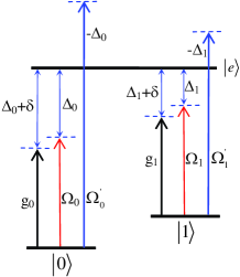
Figure 1: Atomic level structure and couplings. The transition $\left|m\right\rangle(m=0,1)\leftrightarrow$ $\left|e\right\rangle$ is coupled to the cavity mode with strength $g_{m}$ and driven by classical field lasers with Rabi frequency $\Omega_{m}/\Omega_{m}^{\prime}$.

The coupling between the cavity fields and the fiber modes can be written as the interaction Hamiltonian SMB

$$H_{cf}=\underset{i=1}{\overset{\infty}{\sum}}\nu_{i}\left[b_{i}\left(a_{1}^{{\dagger}}+\left(-1\right)e^{i\varphi}a_{2}^{{\dagger}}\right)+\text{H.c.}\right],$$ (1)

where $\nu_{i}$ is the coupling strength between fiber mode $i$ and the cavity mode, $b_{i}$ is the annihilation operator for the fiber mode $i$ while $a_{1}^{{\dagger}}\left(a_{2}^{{\dagger}}\right)$ is the creation operator for the cavity mode $j$($k$), and $\varphi$ is the phase induced by the propagation of the field through the fiber. In the short fiber limit, only resonant mode $b$ of the fiber interacts with the cavity mode. In this case, the Hamiltonian $H_{cf}$ can be approximately written as SMB

$$H_{cf}=\nu\left[b\left(a_{1}^{{\dagger}}+a_{2}^{{\dagger}}\right)+H.c.\right],$$ (2)

where the phase $\left(-1\right)e^{i\varphi}$ in $H_{cf}$ has been absorbed into $a_{2}^{{\dagger}}$ and $a_{2}$ chen_song .

To implement the geometric entangling gate, we let the classical laser fields plotted in Fig. 1 individually act on both atoms $j_{1}$ and $k_{1}$. In the interaction picture, the Hamiltonian describing the atom-field interaction takes the form

$$H_{AC} =\underset{l=j_{1},k_{1}}{\sum}\underset{m=0,1}{\sum}\frac{\Omega_{m}^{\prime}}{2}e^{-i\Delta_{m}t}\left|e\right\rangle_{l}\left\langle m\right|+\frac{\Omega_{m}}{2}e^{i\Delta_{m}t}\left|e\right\rangle_{l}\left\langle m\right|+\underset{l=j_{1},j_{2}}{\sum}\underset{m=0,1}{\sum}g_{m}\left|e\right\rangle_{l}\left\langle m\right|a_{1}e^{i\left(\Delta_{m}+\delta\right)t}$$

$$+\underset{l=k_{1},k_{2}}{\sum}\underset{m=0,1}{\sum}g_{m}\left|e\right\rangle_{l}\left\langle m\right|a_{2}e^{i\left(\Delta_{m}+\delta\right)t}+\text{H.c.}$$ (3)

Following Ref. SMB , we define three bosonic modes $c_{0}=\frac{1}{\sqrt{2}}\left(a_{1}-a_{2}\right)$, $c_{1}=\frac{1}{2}\left(a_{1}+a_{2}+\sqrt{2}b\right)$, $c_{2}=\frac{1}{2}\left(a_{1}+a_{2}-\sqrt{2}b\right)$, $c_{n}(n=0,1,2)$ are linearly relative to the field modes of the cavities and fiber. Then we can rewrite the whole Hamiltonian in the interaction picture as

$$H=H_{0}+H_{i},$$ (4)

where

$$H_{0}=\sqrt{2}\nu c_{1}^{{\dagger}}c_{1}-\sqrt{2}\nu c_{2}^{{\dagger}}c_{2},$$ (5)

and

$$H_{i} =\underset{m=0,1}{\underset{l=j_{1},k_{1}}{\sum}}\frac{\Omega_{m}^{\prime}}{2}e^{-i\Delta_{m}t}\left|e\right\rangle_{l}\left\langle m\right|+\frac{\Omega_{m}}{2}e^{i\Delta_{m}t}\left|e\right\rangle_{l}\left\langle m\right|+\underset{m=0,1}{\underset{l=j_{1},j_{2}}{\sum}}g_{m}\left|e\right\rangle_{l}\left\langle m\right|\frac{1}{2}\left(c_{1}+c_{2}+\sqrt{2}c_{0}\right)e^{i\left(\Delta_{m}+\delta\right)t}$$

$$+\underset{m=0,1}{\underset{l=k_{1},k_{2}}{\sum}}g_{m}\left|e\right\rangle_{l}\left\langle m\right|\frac{1}{2}\left(c_{1}+c_{2}-\sqrt{2}c_{0}\right)e^{i\left(\Delta_{m}+\delta\right)t}+\text{H.c.}$$ (6)

        We now perform the unitary transformation $e^{iH_{0}t}$, and obtain ZhengSB

$$H_{i}= \underset{m=0,1}{\underset{l=j_{1},k_{1}}{\sum}}\left(\frac{\Omega_{m}^{\prime}}{2}e^{-i\Delta_{m}t}\left|e\right\rangle_{l}\left\langle m\right|+\frac{\Omega_{m}}{2}e^{i\Delta_{m}t}\left|e\right\rangle_{l}\left\langle m\right|\right)+\underset{m=0,1}{\underset{l=j_{1},j_{2}}{\sum}}g_{m}\left|e\right\rangle_{l}\left\langle m\right|\frac{1}{2}\left(c_{1}e^{-i\sqrt{2}\nu t}+c_{2}e^{i\sqrt{2}\nu t}+\sqrt{2}c_{0}\right)e^{i\left(\Delta_{m}+\delta\right)t}$$

$$+\underset{m=0,1}{\underset{l=k_{1},k_{2}}{\sum}}g_{m}\left|e\right\rangle_{l}\left\langle m\right|\frac{1}{2}\left(c_{1}e^{-i\sqrt{2}\nu t}+c_{2}e^{i\sqrt{2}\nu t}-\sqrt{2}c_{0}\right)e^{i\left(\Delta_{m}+\delta\right)t}+\text{H.c.}$$ (7)

Here we assume that $\Delta_{m}\gg\sqrt{2}\nu,\delta,g_{m}$ and $\Omega_{m}$ to make sure that atoms cannot exchange energy with the fiber mode, cavity modes, and classical fields on account of the large detuning. In this case, we may adiabatically eliminate the excited atomic state considering no population transferred to the this state. In order to cancel the Stark shifts caused by classical laser fields, we set $\left|\Omega_{m}\right|=\left|\Omega_{m}^{\prime}\right|$. Assuming further $g_{m}\ll\Omega_{m}$, we can neglect the terms of $g_{m}^{2}$, which indicate the Stark shifts caused by bosonic modes. From the above, we obtain an effective Hamiltonian describing the coupling between the atoms and bosonic modes assisted by the classical fields JM

$$H_{eff} =\left(\left|0\right\rangle_{j_{1}}\left\langle 0\right|+\left|0\right\rangle_{k_{1}}\left\langle 0\right|\right)\lambda_{1}e^{-i\left(\delta-\sqrt{2}\nu\right)t}c_{1}^{{\dagger}}+\left(\left|0\right\rangle_{j_{1}}\left\langle 0\right|+\left|0\right\rangle_{k_{1}}\left\langle 0\right|\right)\lambda_{2}e^{-i\left(\delta+\sqrt{2}\nu\right)t}c_{2}^{{\dagger}}$$

$$+\left(\left|0\right\rangle_{j_{1}}\left\langle 0\right|-\left|0\right\rangle_{k_{1}}\left\langle 0\right|\right)\lambda_{0}e^{-i\delta t}c_{0}^{{\dagger}}+\left(\left|1\right\rangle_{j_{1}}\left\langle 1\right|+\left|1\right\rangle_{k_{1}}\left\langle 1\right|\right)\lambda_{1}^{\prime}e^{-i\left(\delta-\sqrt{2}\nu\right)t}c_{1}^{{\dagger}}$$

$$+\left(\left|1\right\rangle_{j_{1}}\left\langle 1\right|+\left|1\right\rangle_{k_{1}}\left\langle 1\right|\right)\lambda_{2}^{\prime}e^{-i\left(\delta+\sqrt{2}\nu\right)t}c_{2}^{{\dagger}}+\left(\left|1\right\rangle_{j_{1}}\left\langle 1\right|-\left|1\right\rangle_{k_{1}}\left\langle 1\right|\right)\lambda_{0}^{\prime}e^{-i\delta t}c_{0}^{{\dagger}}+\text{H.c.,}$$ (8)

where

$\ \ \ \ \ \ \lambda_{0}=-\frac{\sqrt{2}\Omega_{0}g_{0}^{\ast}}{8}\left(\frac{1}{\Delta_{0}}+\frac{1}{\Delta_{0}+\delta}\right)$, $\ \ \ \ \ \ \lambda_{1}=-\frac{\Omega_{0}g_{0}^{\ast}}{8}\left(\frac{1}{\Delta_{0}}+\frac{1}{\Delta_{0}+\delta-\sqrt{2}\nu}\right)$, $\ \ \ \ \ \ \lambda_{2}=-\frac{\Omega_{0}g_{0}^{\ast}}{8}\left(\frac{1}{\Delta_{0}}+\frac{1}{\Delta_{0}+\delta+\sqrt{2}\nu}\right)$,

$\ \ \ \ \ \ \lambda_{0}^{\prime}=-\frac{\sqrt{2}\Omega_{1}g_{1}^{\ast}}{8}\left(\frac{1}{\Delta_{1}}+\frac{1}{\Delta_{1}+\delta}\right)$, $\ \ \ \ \ \ \lambda_{1}^{\prime}=-\frac{\Omega_{1}g_{1}^{\ast}}{8}\left(\frac{1}{\Delta_{1}}+\frac{1}{\Delta_{1}+\delta-\sqrt{2}\nu}\right)$,      $\ \lambda_{2}=-\frac{\Omega_{1}g_{1}^{\ast}}{8}\left(\frac{1}{\Delta_{1}}+\frac{1}{\Delta_{1}+\delta+\sqrt{2}\nu}\right)$.

Because the logical qubits $j$ and $k$ are located at different cavities, the available DFS for the whole system is constructed by $\mathcal{C}_{jk}^{4}\equiv\mathcal{C}_{j}^{2}\otimes\mathcal{C}_{k}^{2}=\left\{\left|0_{j}^{L}0_{k}^{L}\right\rangle\text{, }\left|0_{j}^{L}1_{k}^{L}\right\rangle\text{, }\left|1_{j}^{L}0_{k}^{L}\right\rangle\text{, }\left|1_{j}^{L}1_{k}^{L}\right\rangle\right\},$ and in this DFS the Hamiltonian $H_{eff}$ is diagonal and takes the form

$$H_{eff}=diag\left[H_{0_{j}0_{k}}\text{, }H_{0_{j}1_{k}}\text{, }H_{1_{j}0_{k}}\text{, }H_{1_{j}1_{k}}\right],$$ (9)

where the diagonal matrix elements $H_{\mu_{j}\nu_{k}}(\mu,$ $\nu=0,1)$ are of the form

$$H_{\mu_{j}\nu_{k}}=\underset{n=0}{\overset{2}{\sum}}c_{n}^{{\dagger}}\chi_{\mu_{j}\nu_{k}}^{n}e^{-i\eta_{n}t}+\text{H.c.,}$$ (10)

where

$\ \ \ \chi_{0_{j}0_{k}}^{0}=0$, $\chi_{0_{j}0_{k}}^{1}=2\lambda_{1}$, $\chi_{0_{j}0_{k}}^{2}=2\lambda_{2}$; $\ \ \ \chi_{0_{j}1_{k}}^{0}=\lambda_{0}-\lambda_{0}^{\prime}$, $\chi_{0_{j}1_{k}}^{1}=\lambda_{1}+\lambda_{1}^{\prime}$, $\chi_{0_{j}1_{k}}^{2}=\lambda_{2}+\lambda_{2}^{\prime}$;

$\ \ \ \chi_{1_{j}0_{k}}^{0}=\lambda_{0}^{\prime}-\lambda_{0}$, $\chi_{1_{j}0_{k}}^{1}=\lambda_{1}+\lambda_{1}^{\prime}$, $\chi_{1_{j}0_{k}}^{2}=\lambda_{2}+\lambda_{2}^{\prime}$;    $\chi_{1_{j}1_{k}}^{0}=0$, $\chi_{1_{j}1_{k}}^{1}=2\lambda_{1}^{\prime}$, $\chi_{0_{j}0_{k}}^{2}=2\lambda_{2}^{\prime}$.
and

$\eta_{0}=\delta$, $\eta_{1}=\delta-\sqrt{2}\nu$, $\eta_{2}=\delta+\sqrt{2}\nu$.

Obviously, in the DFS $\mathcal{C}_{jk}^{4}$, time evolution matrix $U\left(t\right)$ also takes a diagonal form,

$$U\left(t\right)=diag\left[U_{0_{j}0_{k}}\text{, }U_{0_{j}1_{k}}\text{, }U_{1_{j}0_{k}}\text{, }U_{1_{j}1_{k}}\right].$$ (11)

The corresponding diagonal matrix elements$\ U_{\mu_{j}\nu_{k}}\left(t\right)$ can be derived from Eq. (10) and they are in terms of displacement operator

$$\ U_{\mu_{j}\nu_{k}}\left(t\right) =\hat{T}\exp\left[-i\int_{0}^{t}H_{\mu_{j}\nu_{k}}\left(\tau\right)d\tau\right]=\underset{n=0}{\overset{2}{\prod}}\exp\left({i\phi_{\mu_{j}\nu_{k}}^{n}}\right)D\left(\int_{c}d\alpha_{\mu_{j}\nu_{k}}^{n}\right)=\exp\left[{i}\phi_{\mu_{j}\nu_{k}}\right]\underset{n=0}{\overset{2}{\prod}}D\left(\int_{c}d\alpha_{\mu_{j}\nu_{k}}^{n}\right)\ ,$$ (12)

  

with $\hat{T}$ being the time ordering operator, and

$$\phi_{\mu_{j}\nu_{k}}=\overset{2}{\underset{n=0}{\sum}}\phi_{\mu_{j}\nu_{k}}^{n}=\overset{2}{\underset{n=0}{\sum}}\operatorname{Im}\left[\int_{c}\left(\alpha_{\mu_{j}\nu_{k}}^{n}\right)^{\ast}d\alpha_{\mu_{j}\nu_{k}}^{n}\right],$$ (13)

$$d\alpha_{\mu_{j}\nu_{k}}^{n}=-i\chi_{\mu_{j}\nu_{k}}^{n}e^{-i\eta_{n}\tau}d\tau$$ (14)

Considering the situation, where each bosonic mode is assumed initially in vacuum state, the state of each bosonic mode evolves to coherent state at time $t_{n}>0$. The corresponding amplitude $\int_{c}d\alpha_{\mu_{j}\nu_{k}}^{n}$ is dependent on the logic computational basis state $\left|\mu_{j}^{L}\nu_{k}^{L}\right\rangle$. It is not difficult to obtain $\alpha_{\mu_{j}\nu_{k}}^{n}$ by integrating Eq. (14)

$$\alpha_{\mu_{j}\nu_{k}}^{n}=\frac{\chi_{\mu_{j}\nu_{k}}^{n}}{\eta_{n}}\left(e^{-i\eta_{n}t}-1\right).$$ (15)

The above equation indicates that there is a time period $T$ fulfilling the relation $T=2\pi l_{n}/\eta_{n}$, where $l_{n}$ is a positive integer and $n=0,1,2$, in which the bosonic mode $c_{n}$ completes $l_{n}$ evolutions and returns to its initial vacuum state. During this process the system accumulates the following total phase

$$\gamma_{\mu_{j}\nu_{k}}(T) =\phi_{\mu_{j}\nu_{k}}(T)=-\overset{2}{\underset{n=0}{\sum}}\frac{2\pi l_{n}}{\eta_{n}}\left|\chi_{\mu_{j}\nu_{k}}^{n}\right|^{2}=\gamma_{\mu_{j}\nu_{k}}^{g}+\gamma_{\mu_{j}\nu_{k}}^{d},$$ (16)

where $\gamma_{\mu_{j}\nu_{k}}^{d}$ and $\gamma_{\mu_{j}\nu_{k}}^{g}$ stand for the dynamical and geometric phases respectively, and can be calculated by using the coherent state path integral method MH

$$\gamma_{\mu_{j}\nu_{k}}^{d} =\overset{2}{\underset{n=0}{\sum}}-\int_{0}^{T}H_{\mu_{j}\nu_{k}}^{n}\left(\left(\alpha_{\mu_{j}\nu_{k}}^{n}\right)^{\ast},\alpha_{\mu_{j}\nu_{k}}^{n};t\right)dt=-\overset{2}{\underset{n=0}{\sum}}\frac{4\pi l_{n}}{\eta_{n}^{2}}\left|\chi_{\mu_{j}\nu_{k}}^{n}\right|^{2},$$ (17)

$$\gamma_{\mu_{j}\nu_{k}}^{g}=\gamma_{\mu_{j}\nu_{k}}-\gamma_{\mu_{j}\nu_{k}}^{d}=\overset{2}{\underset{n=0}{\sum}}\frac{2\pi l_{n}}{\eta_{n}^{2}}\left|\chi_{\mu_{j}\nu_{k}}^{n}\right|^{2},$$ (18)

we find $\gamma_{\mu_{j}\nu_{k}}=-\gamma_{\mu_{j}\nu_{k}}^{g}=\frac{1}{2}\gamma_{\mu_{j}\nu_{k}}^{d}$. Thus the total phase $\gamma_{\mu_{j}\nu_{k}}$ and dynamical phase $\gamma_{\mu_{j}\nu_{k}}^{d}$ possess global geometric features as does the geometric phase $\gamma_{\mu_{j}\nu_{k}}^{g}$. Therefore at time $t=T=2\pi l_{n}/\eta_{n}$ the time evolution matrix takes the form

$$U\left(T\right)=diag\left[e^{i\gamma_{0_{j}0_{k}}}\text{, }e^{i\gamma_{0_{j}1_{k}}}\text{, }e^{i\gamma_{1_{j}0_{k}}}\text{, }e^{i\gamma_{1_{j}1_{k}}}\text{ }\right].$$ (19)

$U\left(T\right)$ is actually the geometric entangling gate operation we are targeting at and $U\left(T\right)$ is a nontrivial entangling gate when the condition $\gamma_{0_{j}0_{k}}+\gamma_{1_{j}1_{k}}\neq\gamma_{0_{j}1_{k}}+\gamma_{1_{j}1_{k}}$ is fulfilled X .

We now give a brief discussion about the decoherence mechanisms of our scheme: atomic spontaneous emission, cavity decay and fiber loss. Considering none of the atoms are initially populated in the excited state since the quantum information is encoded in ground states, and atoms cannot exchange energy with the fiber mode, cavity modes and classical fields due to the large detuning, thus no population is transferred to the excited atomic state. In this sense, the spontaneous emission of the atomic excited state can be ignored.

Regarding the cavity decay and the fiber loss, the fidelity of the resulting gates will be greatly impaired by them because the geometric phases are acquired by the evolution of the optical modes. So, strictly speaking, our scheme requires ideal good cavities and fiber. However, if the mean number of photons of the optical fields is sufficiently small, the cavities and fiber are normally not excited and the moderate cavity decay and fiber loss can thus be tolerated. For a coherent state the mean number of photons is equal to the square of the amplitude of the state which is determined by Eq.(15). Thus when the condition $\frac{\chi_{\mu_{j}\nu_{k}}^{n}}{\eta_{n}}\ll 1$ is fulfilled CQED1 , the mean number of photons of the coherent state is an even smaller number and can be regarded as a sufficiently small number to ignore the effect of cavity and fiber decay. Now let us use an example for further explanation. We choose the following experimentally achievable parameters Kimble $\nu/2\pi=26.72$ MHz, $g_{0}/2\pi=g_{1}/2\pi=20$ MHz, $\Omega_{0}/2\pi=\Omega_{1}/2\pi=120$ MHz, $\Delta_{0}/2\pi=3000$ MHz, $\Delta_{1}/2\pi=600$ MHz, $\delta/2\pi=35$ MHz. These parameters satisfy the requirement $\frac{\chi_{\mu_{j}\nu_{k}}^{n}}{\eta_{n}}\ll 1$ and the approximation conditions adopted in our derivation. The resulting entangling gate corresponding to these parameters is $U(t)=diag\left\{e^{0.1248i},e^{1.056i},e^{1.056i},e^{i\pi}\right\}$ with the gate operation time $t\approx 0.3448$ $\mu$s. Obviously the gate operation time is much shorter than the photon lifetime in optical cavities AA . According to Eq. (15) the amplitude of the coherent state is dependent on the atomic states, for the above parameters the amplitude corresponding to state $\left|1_{j}^{L}1_{k}^{L}\right\rangle$ takes the maximal value, and the maximal mean number of photons is 0.1087. In this case, the optical modes are hardly excited and thus the moderate cavity decay and fiber loss can be tolerated.

In conclusion, we have proposed a scheme to implement geometric entangling gates for two logical qubits in a coupled cavity system in DFS. Our scheme possesses both advantages of DFS and the geometric phase. Besides, in comparison with the scheme of Ref. X which works in a single cavity, the scheme proposed in this paper can easily realize the scalability of cavity QED-based quantum computing by using the idea of the distributed quantum computingJA and can relax the requirement for individually addressing atoms.

The work is supported by the NSFC under Grant No. 11074079, the Ph.D. Programs Foundation of Ministry of Education of China, the Open Fund of the State Key Laboratory of High Field Laser Physics ( Shanghai Institute of Optics and Fine Mechanics), and National Research Foundation and Ministry of Education, Singapore, under research Grant No. WBS: R-710-000-008-271.

References

• (1) A. Serafini, S. Mancini, and S. Bose Phys. Rev. Lett. 96 (2006) 010503.
• (2) L.-B. Chen, M.-Y. Ye, G.-W. Lin, Q.-H. Du, and X.-M. Lin, Phys. Rev. A 76 (2007) 062304; J. Song, Y. Xia, H.-S. Song, J.-L. Guo, J. Nie Europhysics Lett. 80 (2007) 60001.
• (3) S.-B. Zheng, Appl. Phys. Lett. 94 (2009) 154101.
• (4) J. I. Cirac et al., Phys. Rev. Lett. 78 (1997) 3221; S. J.van Enk et al., ibid. 79 (1997) 5178.
• (5) S. J. van Enk et al., Phys. Rev. A 59 (1999) 2659.
• (6) S. Clark et al., Phys. Rev. Lett. 91 (2003) 177901.
• (7) S. Bose et al., Phys. Rev. Lett. 83 (1999) 5158; S.Manciniand S. Bose, Phys. Rev. A 64 (2001) 032308; D. E.Browne et al., Phys. Rev. Lett. 91 (2003) 067901.
• (8) L.M. Duan and H. J. Kimble, Phys. Rev. Lett. 90 (2003) 253601.
• (9) G. M. Palma, K. Suominen, and A. K. Ekert, Proc. R. Soc. A 452 (1996) 567; L.-M. Duan and G.-C. Guo, Phys. Rev. Lett. 79 (1997) 1953; P. Zanardi and M. Rasetti, ibid. 79 (1997) 3306; D. A. Lidar, I. L. Chuang, and K. B. Whaley, ibid. Phys. Rev. Lett. 81 (1998) 2594.
• (10) P. W. Shor, Phys. Rev. A 52 (1995) R2493.
• (11) P. Zanardi and M. Rasetti, Phys. Lett. A 264 (1999) 94.
• (12) J. A. Jones, V. Vedral, A. Ekert, and G. Castagnoli, Nature (London) 403 (2000) 869; G. Falci, R. Fazio, G. M. Palma, J. Siewert, and V. Vedral, ibid 407 (2000) 355; X.-B. Wang and M. Keiji, Phys. Rev. Lett. 87 (2001) 097901.
• (13) L.M. Duan, J. I. Cirac, and P. Zoller, Science 292 (2001) 1695.
• (14) X. Wang and P. Zanardi, Phys. Rev. A 65 (2002) 032327.
• (15) S.-L. Zhu and Z.D. Wang, Phys. Rev. Lett. 91 (2003) 187902.
• (16) S. B. Zheng, Phys. Rev. A 70 (2004) 052320.
• (17) X.-L. Feng, Z. Wang, C. Wu, L.C. Kwek, C. H. Lai, and C. H. Oh, Phys. Rev. A 75 (2007) 052312.
• (18) L.-X. Cen, Z. D. Wang, and S. J. Wang, Phys. Rev. A 74 (2006) 032321.
• (19) X.-L. Feng, C. Wu, H. Sun, and C.H. Oh, Phys. Rev. Lett. 103 (2009) 200501.
• (20) J. I. Cirac, A. K. Ekert, S. F. Huelga and C. Macchiavello, Phys. Rev. A 59 (1999) 4249.
• (21) D. F. V. James, Fortschr. Phys. 48 (2000) 823.
• (22) Mark Hillery, M. S. Zubairy, Phys. Rev. A 26(1982) 451.
• (23) A. D. Boozer, A. Boca, R. Miller, T. E. Northup, and H. J. Kimble, Phys. Rev. Lett. 97 (2006) 083602.
• (24) A. A. Savchenkov, A. B.Matsko, V. S. Ilchenko, and L.Maleki, Opt. Express 15 (2007) 6768.