Particle-hole bound states of dipolar molecules in optical lattice

Abstract

We investigate the particle-hole pair excitations of dipolar molecules in optical lattice, which can be described with an extended Bose-Hubbard model. For strong enough dipole-dipole interaction, the particle-hole pair excitations can form bound states in one and two dimensions. With decreasing dipole-dipole interaction, the energies of the bound states increase and merge into the particle-hole continuous spectrum gradually. The existence regions, the energy spectra and the wave functions of the bound states are carefully studied and the symmetries of the bound states are analyzed with group theory. For a given dipole-dipole interaction, the number of bound states varies in momentum space and a number distribution of the bound states is illustrated. We also discuss how to observe these bound states in future experiments.

I Introduction

Cold and ultracold molecules are attracting more and more attention due to their broad applications in the fields of high-precision measurement, quantum chemistry, quantum information and many-body physics molecule-review . Recent years the experimental techniques for cold and ultracold molecules have been developed greatly. The homonuclear molecular Bose-Einstein condensation (BEC) was realized experimentally Jochim ; Greiner and the quantum state with exactly one molecule at each site of an optical lattice was created with a Feshbach resonance and STIRAP (stimulated Raman adiabatic passage) techniques Volz ; Danzl1 . Meanwhile the ultracold heteronuclear molecules were also produced Sage ; Wang ; Sawyer ; Ni ; Ospelkaus .

The heteronuclear molecules, such as SrO, RbCs, or NaCs, prepared in their electronic and vibrational ground states, have considerable permanent electric dipole moment. The dipole-dipole interaction between molecules can be generated by the external applied electric field molecule-review . Moreover, the magnitude of the dipole-dipole interaction can be controlled by the strength of the electric field DeMille ; buchler . The tunable long range dipole-dipole interaction may significantly modify the ground state and collective excitations of trapped condensates. For example, in trapped dipolar gases, it was shown theoretically Santos that the mean-field inter-particle interaction and, hence, the stability diagram are governed by the trapping geometry. With increasing dipolar interaction, the ground state of rotating atomic Bose gases undergoes a series of transitions between vortex lattices of different symmetries: triangular, square, “stripe”, and “bubble” phases Cooper . In rapidly rotating Fermion gas, the dipole-dipole interaction may even result in the fractional quantum Hall-like states Baranov05 .

The particles with long-range interactions in optical lattice can be described with extended Hubbard model goral ; Menotti ; Lin . Compared with the regular Bose-Hubbard model with on-site interaction, the extended Bose-Hubbard model has richer ground state phases, such as Mott insulator, particle density wave, superfluidity or supersolid phase Bruder ; Otterlo ; Niyaz ; Sengupta ; Hassan ; Iskin ; PAI ; Chen . On the other hand, the gapful particle and hole excitations in the insulating phase fisher ; stoof ; Kovrizhin may bind together and form bound states due to the long-range interactions. Although the excitons (holon-doublon pairs) in one-dimensional fermionic Hubbard model have been extensively studied fermion-exciton , the excitons in higher dimensions, and especially, in bosonic Hubbard models are less studied.

In this paper, we study the particle-hole pair excitations of dipolar bosonic molecules in optical lattice, especially, the possible bound states due to the dipole-dipole interaction. The paper is organized as follows. In Sec. II we introduce the extended Bose-Hubbard model to describe the polarized bosonic molecules in optical lattice, and derive the eigen equations to describe the single particle-hole pair excitation. In Sec. III, the existence regions, the energies and the wave functions of the particle-hole bound states are calculated in one and two dimensions. The symmetries of the bound states are analyzed and possible experimental observation of these bound states is also discussed. A summary is presented in Sec. IV.

II The particle-hole bound states in the extended Bose-Hubbard model

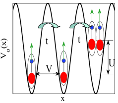
Figure 1: Sketches of optical lattice and interactions of ultracold heteronuclear molecules. (a) The landscape of optical lattice potential in the x-y plane. The square optical lattice potential $V_{o}(x,y)=V_{opt}[sin^{2}(k_{x}x)+sin^{2}(k_{y}y)]$ can be created by counter propagating far detuned laser beams, where $V_{opt}$ is the depth of lattice and $k_{x(y)}$ is the laser wave vector along $x(y)$ direction. (b) The interactions between dipolar molecules in the optical lattice (see equation(1)). The arrows on the molecules indicate the polarization of the electric dipole moments.

Considering only the nearest-neighbor interaction V to simulate the effect of dipole-dipole interaction, we write the extended Bose-Hubbard model as,

$$H=H_{0}+H_{1},$$

$$H_{0}=\frac{U}{2}\sum_{\vec{r}}n_{\vec{r}}(n_{\vec{r}}-1)+\frac{V}{2}\sum_{\vec{r},\vec{\sigma}}n_{\vec{r}}n_{\vec{r}+\vec{\sigma}},$$

$$H_{1}={-t}\sum_{\vec{r},\vec{\sigma}}(b_{\vec{r}}^{\dagger}b_{\vec{r}+\vec{\sigma}}),$$ (1)

where $n_{\vec{r}}=b_{\vec{r}}^{{\dagger}}b_{\vec{r}}$ is the number operator at site $\vec{r}$ with $b_{\vec{r}}(b_{\vec{r}}^{{\dagger}})$ the annihilation (creation) operator of particle. $\vec{\sigma}$ denotes the nearest neighbor vectors of site $\vec{r}$. The on-site interaction $U$, the nearest neighbor interaction $V$ and the hopping $t$ are expressed as

$$U = g\int d\vec{x}|W(\vec{x})|^{4},$$

$$V = \int d\vec{x}d\vec{x}^{\prime}|W(\vec{x}-\vec{r})|^{2}V_{dd}(\vec{x}-\vec{x}^{\prime})|W(\vec{x}^{\prime}-(\vec{r}+\vec{\sigma}))|^{2},$$

$$t = -\int d\vec{x}W^{\ast}(\vec{x}-\vec{r})(-\frac{\hbar^{2}}{2m}\nabla^{2}+V_{0}(\vec{x}))W(\vec{x}-(\vec{r}+\vec{\sigma})),$$

where $W(\vec{r})$ is Wannier function corresponding to the lowest energy band and $V_{dd}(\vec{x})=\frac{C_{dd}}{4\pi}\frac{1-3cos^{2}\theta}{|\vec{x}|^{3}}$ is the dipole-dipole interaction of two particles separated with a distance $|\vec{x}|$. For the electric dipole-dipole interaction, $C_{dd}=\frac{d^{2}}{\epsilon_{0}}$ with $d$ the electric dipole moment, $\epsilon_{0}$ is vacuum permittivity. We assume that the polarization of dipole moment is along the $z$ axial direction. In the following studies, we consider particles confined in one-dimensional chain or two-dimensional square lattice and treat hopping term $H_{1}$ as a perturbation.

In the atomic limit ($t=0$), $n_{\vec{r}}$ is a good quantum number and the eigenstates of $H_{0}$ can be written as direct product of number states. When the filling factor is one, $V\geq 0$ and $zV<U$, the Mott insulating ground state can be written as $|11111111...\rangle$ with the ground state energy $E_{0}={\frac{1}{2}}NzV$, where z is the coordination number and N the number of lattice sites. The excited states contain one or more particle-hole pairs. A single particle-hole pair state with a hole at $r$ and a particle at $r^{\prime}$ can be represented as $|r,r^{\prime}\rangle=|110_{r}111112_{r^{\prime}}11...\rangle$. Taking into account the hopping term $t$, the particle and hole will move in the lattice. Similar to the two-magnon states in ferromagnetic system mattis , the single particle-hole pair state can be written as a linear combination of $|r,r^{\prime}\rangle$:

$$|\psi\rangle=\sum_{\vec{r},\vec{r}\prime}\phi_{\vec{r},\vec{r}\prime}|\vec{r},\vec{r}\prime\rangle,$$ (3)

where $\phi_{\vec{r},\vec{r}^{\prime}}$ will be determined by solving the approximate eigen equation in single particle-hole pair subspace

$$\langle\vec{r},\vec{r}\prime|H|\psi\rangle=E\langle\vec{r},\vec{r}\prime|\psi\rangle.$$ (4)

Calculating $H|\vec{r},\vec{r}^{\prime}\rangle$ and considering the boundary condition $\phi_{\vec{r},\vec{r}}=0$ (a particle and a hole do not share the same lattice site), we get

$$-\sum_{\vec{\sigma}}(t\phi_{\vec{r}+\vec{\sigma},\vec{r}^{\prime}}+2t\phi_{\vec{r},\vec{r}^{\prime}+\vec{\sigma}})=\varepsilon\phi_{\vec{r},\vec{r}^{\prime}}$$

$$+\sum_{\vec{\sigma}}\delta_{\vec{r}^{\prime}-\vec{r},\vec{\sigma}}[V\phi_{\vec{r},\vec{r^{\prime}}}+(-t)\phi_{\vec{r}+\vec{\sigma},\vec{r^{\prime}}}+(-2t)\phi_{\vec{r},\vec{r^{\prime}}-\vec{\sigma}}]$$

$$-\delta_{\vec{r}^{\prime}-\vec{r},0}\sum_{\vec{\sigma}}(t\phi_{\vec{r}+\vec{\sigma},\vec{r}^{\prime}}+2t\phi_{\vec{r},\vec{r}^{\prime}+\vec{\sigma}}),$$ (5)

where $\delta_{\vec{r}^{\prime}-\vec{r},\sigma}$ is the Kronecker delta function and $\varepsilon=E-E_{0}-U$. The particle-hole excitation energy is $\omega=E-E_{0}=\varepsilon+U$.

Owing to the translational invariance, it is convenient to apply a transformation $\phi_{\vec{r},\vec{r}^{\prime}}=\frac{1}{\sqrt{N}}e^{i\vec{K}\cdot\vec{R}}\phi(\vec{\rho})$, where $\vec{R}=\frac{\vec{r}+\vec{r}^{\prime}}{2}$ and $\vec{\rho}=\vec{r}^{\prime}-\vec{r}$ denote the center-of-mass and the relative coordinates respectively and $\vec{K}$ the total momentum of the particle and hole. At fixed $\vec{K}$, the eigen equation $(5)$ becomes

$$-\sum_{\vec{\sigma}}[te^{i\frac{\vec{K}\cdot\vec{\sigma}}{2}}\phi(\vec{\rho}-\vec{\sigma})+2te^{i\frac{\vec{K}\cdot\vec{\sigma}}{2}}\phi(\vec{\rho}+\vec{\sigma})]=$$

$$\varepsilon\phi(\vec{\rho})+\sum_{\vec{\sigma}}\delta_{\vec{\rho},\vec{\sigma}}[V\phi(\vec{\rho})+(-te^{i\frac{\vec{K}\cdot\vec{\sigma}}{2}}-2te^{i\frac{-\vec{K}\cdot\vec{\sigma}}{2}})\phi(\vec{\rho}-\vec{\sigma})]$$

$$-\delta_{\vec{\rho},0}\sum_{\vec{\sigma}}[te^{-i\frac{\vec{K}\cdot\vec{\sigma}}{2}}\phi(\vec{\sigma})+2te^{i\frac{\vec{K}\cdot\vec{\sigma}}{2}}\phi(\vec{\sigma})].$$ (6)

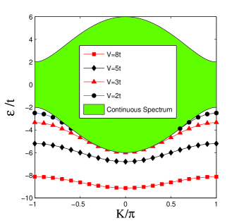
Figure 2: Energy spectra of the bound states of particle-hole pair in one dimension for different nearest-neighbor interactions $V=2t$ (black circles), $V=3t$ (red triangles), $V=5t$ (black diamonds) and $V=8t$ (red squares) respectively ($K=K_{x}$). As comparison, the continuous spectrum of a particle-hole pair excitation is also shown (green shaded region).

Considering the finite range character of the nearest neighbor interaction $V$, we utilize the Green’s function approach to solve the eigen equation. To this end, we introduce an effective Hamiltonian

$$H_{eff}=H_{ph,0}+V_{ph},$$ (7)

where

$$H_{ph,0} = -t\sum_{\vec{\rho},\vec{\sigma}}e^{i\vec{K}\cdot\vec{\sigma}/2}|\vec{\rho}\rangle\langle\vec{\rho}-\vec{\sigma}|-2te^{i\vec{K}\cdot\vec{\sigma}/2}|\vec{\rho}\rangle\langle\vec{\rho}+\vec{\sigma}|,$$

$$V_{ph} = \sum_{\vec{\sigma}}(2te^{-i\vec{K}\cdot\vec{\sigma}/2}+te^{i\vec{K}\cdot\vec{\sigma}/2})|\vec{\sigma}\rangle\langle 0|+h.c.$$

$$+ \sum_{\vec{\sigma}}(-V)|\vec{\sigma}\rangle\langle\vec{\sigma}|,$$

to describe the motion of a particle around a hole, where $|\vec{\rho}\rangle$ is basis set in relative coordinate spaces. The $\vec{K}$-dependent $H_{ph,0}$ describes the kinetic energy of the particle and $V_{ph}$ denotes the interaction between particle and hole. With $|\phi\rangle=\sum_{\vec{\rho}}\phi(\vec{\rho})|\vec{\rho}\rangle$, it is easy to reproduce Eq. (6) from the eigen equation $H_{eff}|\phi\rangle=\varepsilon|\phi\rangle$. After a Fourier transformation, the kinetic energy is obtained as

$$\varepsilon_{0}(\vec{K},\vec{q}) = -t\sum_{\vec{\sigma}}e^{i(\vec{K}/2+\vec{q})\cdot{\vec{\sigma}}}-2t\sum_{\vec{\sigma}}e^{i(\vec{K}/2-\vec{q})\cdot{\vec{\sigma}}},$$ (8)

where $\vec{q}$ is the relative momentum of particle and hole. When a particle is adjacent to a hole, the energy offset $-V$ in $V_{ph}$ may result in the formation of particle-hole bound states.

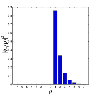
Figure 3: Probability density of a bound state in real space in the case of $V=8t$ and $K=0$. The probability density decreases exponentially with increase of distance.

Introducing retarded Green functions $G_{0}=\lim_{\eta\to 0^{+}}1/(\varepsilon-H_{ph,0}+i\eta)$ and $G=\lim_{\eta\to 0^{+}}1/(\varepsilon-H_{eff}+i\eta)$, we could calculate $G$ through the Lippmann-Schwinger equation $G=G_{0}+G_{0}V_{ph}G$. In the real space, the Green’s function $G$ has a general form

$$\langle\vec{\rho^{\prime}}|G|\vec{\rho}\rangle=\lim_{\eta\to 0^{+}}\sum_{m}\frac{\phi_{m}(\vec{\rho^{\prime}})\phi_{m}^{\ast}(\vec{\rho})}{\varepsilon-E_{m}+i\eta}=G(\vec{\rho^{\prime}},\vec{\rho},\varepsilon),$$

where the contributions of the continuous spectra are neglected and $E_{m}$’s are the eigenvalues of the bound states with $\phi_{m}$’s the corresponding eigenfunctions Economou . We can determine the eigenvalues and eigenfunctions by analyzing the poles and residues of the obtained Green’s function.

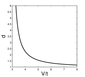
Figure 4: The mean size $d$ of bound states as a function of $V$ at K=0 in one dimension. When the nearest-neighbor interaction $V$ approaches the critical value $V=3t$, the mean size of the bound state becomes divergent and the bound state energies merge into the continuous spectrum (see the red triangles in Fig.2), indicating the disintegration of the bound states.

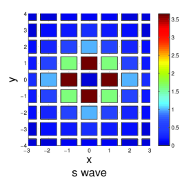
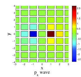
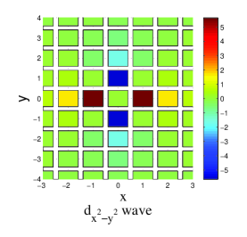
Figure 5: The wave functions of bound states in two dimensional case at $\vec{K}=(0,0)$ and $V=12t$ (non-normalized). $s$-, $p_{x}$- and $d_{x^{2}-y^{2}}$-wave symmetries can be observed respectively.

From Eq. (7), we have

$$\langle\vec{\rho^{\prime}}|G_{0}|\vec{\rho}\rangle=\lim_{\eta\to 0^{+}}\frac{1}{(2\pi)^{d}}\int_{-\pi}^{\pi}\frac{d^{d}qe^{i\vec{q}\cdot(\vec{\rho^{\prime}}-\vec{\rho})}}{\varepsilon-\varepsilon_{0}(\vec{K},\vec{q})+i\eta},$$

and

$$\langle\vec{\rho^{\prime}}|G|\vec{\rho}\rangle = \langle\vec{\rho^{\prime}}|G_{0}|\vec{\rho}\rangle$$ (9)

$$+\sum_{\vec{\rho_{1}},\vec{\rho_{2}}}\langle\vec{\rho^{\prime}}|G_{0}|\vec{\rho_{1}}\rangle\langle\vec{\rho_{1}}|V_{ph}|\vec{\rho_{2}}\rangle\langle\vec{\rho_{2}}|G|\vec{\rho}\rangle.$$

For specific $\vec{\rho\prime}=0$ or $\sigma$, Eq. (9) can be reduced to a set of simultaneous linear equations. Green’s functions $\langle\vec{\rho^{\prime}}|G|\vec{\rho}\rangle$ with $\vec{\rho\prime}=0$ or $\sigma$ can thus be obtained exactly. The residues of $\langle 0|G|\vec{\rho}\rangle$ is always vanishing for non-vanishing bound states energies $\varepsilon$ in our calculations, which is consistent with the boundary condition $\phi(0)=0$. We present our results in the next section.

III bound states in one and two dimensions

III.1 Bound states in one dimension

In the Mott insulating phase, the excitation energy of a single particle/hole was calculated as

$$\omega_{p,h} = \pm[-\frac{\varepsilon_{0}}{2}+U(n_{0}-\frac{1}{2})+2dVn_{0}-\mu]$$ (10)

$$+[(\frac{\varepsilon_{0}}{2})^{2}+\varepsilon_{0}U(n_{0}+\frac{1}{2})+\frac{U^{2}}{4}]^{\frac{1}{2}}$$

with the dynamical Gutzwiller approach Kovrizhin . Up to the first order of $\frac{t}{U}$, the single particle-hole pair excitation energy is

$$\omega=\omega_{p}(\vec{k}_{p})+\omega_{h}(\vec{k}_{h}) = U+\varepsilon_{0}(\vec{K},\vec{q})$$ (11)

with the total momentum $\vec{K}=\vec{k}_{p}+\vec{k}_{h}$ and relative momentum $\vec{q}=(\vec{k}_{h}-\vec{k}_{p})/2$. For the extended Bose-Hubbard model, however, a particle-hole pair may form a bound state due to the interaction (See Eq. (7)). In the following calculations, we take the lattice constant as $1$ and use $t>0$ as the unit of energy. Conditions of $t/U\ll 1$ and $zV<U$ are assumed to make sure that the ground state of the system is the deep Mott insulating phase.

In one dimensional case, $\varepsilon_{0}(\vec{K},\vec{q})=-2t_{\hat{x}}\cos(q+\theta_{x})$ with $t_{\hat{x}}\!\!\!\!=\!\!t\sqrt{9cos^{2}(\frac{K_{x}}{2})+sin^{2}(\frac{K_{x}}{2})}$ and $\theta_{\hat{x}}=arctan(\frac{1}{3}tan(\frac{K_{x}}{2}))$. The top and bottom boundaries of particle-hole continuous spectrum are

$$\Omega_{1}^{t(b)}(K)=\pm 2t_{\hat{x}},$$ (12)

(see Fig.2). Compared with particle-hole pairs in fermion Hubbard model with half filling Barford , the minimum of band width of the continuous spectrum is non-zero at $K=\pm\pi$. This is because that there are no particle-hole symmetries in Bose-Hubbard model.

For a specific nearest-neighbor interaction $V$ and total momentum $K$, we search for bound state solutions outside the continuum. In the case of $\varepsilon<-2t_{\hat{x}}$, the free Green function is calculated as Nygaard

$$\langle\vec{\rho^{\prime}}|G_{0}|\vec{\rho}\rangle = \lim_{\eta\to 0^{+}}\frac{1}{(2\pi)^{d}}\int_{-\pi}^{\pi}\frac{d^{d}qe^{i\vec{q}\cdot(\vec{\rho^{\prime}}-\vec{\rho})}}{\varepsilon-\varepsilon_{0}(\vec{K},\vec{q})+i\eta}$$ (13)

$$= \alpha\beta^{|\rho-\rho^{\prime}|}\gamma^{\rho-\rho^{\prime}},$$

where $\alpha=-\frac{1}{\sqrt{\varepsilon^{2}-4t_{\hat{x}}^{2}}}$, $\gamma=e^{i\theta_{\hat{x}}}$ and $\beta=e^{-\kappa}$ with $\kappa=arccosh(\frac{|\varepsilon|}{2t_{\hat{x}}})$.

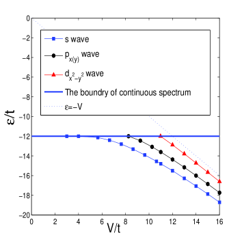
Figure 6: Variations of the energies of different bound states in two dimension at $\vec{K}=(0,0)$. The energies of different bound states increase with decreasing $V$ and cross the particle-hole continuum ($-12t$ at $\vec{K}=(0,0)$) at different $V$.

With $\rho^{\prime}=0$, $\pm 1$, Eq. (9) is reduced to $3$ linear equations. The Green functions of $\langle-1|G|\rho\rangle$, $\langle 0|G|\rho\rangle$ and $\langle 1|G|\rho\rangle$ can be exactly obtained as

$$\langle-1|G|\rho\rangle=\frac{\theta(-\rho)(\beta/\gamma)^{-(\rho+1)}}{-\frac{1}{\beta}(t_{\hat{x}}-V\beta)} \rho\neq 0$$

$$\langle 0|G|\rho\rangle=0,$$

$$\langle 1|G|\rho\rangle=\frac{\theta(\rho)(\beta\gamma)^{\rho-1}}{-\frac{1}{\beta}(t_{\hat{x}}-V\beta)} \rho\neq 0,$$ (14)

where $\theta(\rho)$ is Heaviside step function. From these Green functions, we obtain two degenerate bound states corresponding to the particle on the left (right) of the hole respectively. The bound state energy is

$$\varepsilon=-V-\frac{t_{\hat{x}}^{2}}{V}.$$ (15)

Accordingly, $\beta$ is simplified as $\beta=\frac{t_{\hat{x}}}{V}<1$ and the condition for the existence of the bound state is obtained as

$$V\!\!>\!\!t\sqrt{9cos^{2}(\frac{K_{x}}{2})+sin^{2}(\frac{K_{x}}{2})}.$$ (16)

When $0\leq V\leq t$, the interaction between particle and hole is too weak to bind them together and no bound state is found. When $t<V<3t$, two degenerate bound states exist in the regions of $2arccos\sqrt{\frac{V^{2}-t^{2}}{8t^{2}}}<|K_{x}|\leq\pi$. The region get larger with the increase of $V$. When $V\geq 3t$, bound states may be found in the whole first Brillouin zone. In Fig.2, we show the spectra of the bound states for the interaction $V=2t$, $3t$, $5t$ and $8t,$ respectively. The energies of the bound states decrease with increasing $V$. At $V=2t$, the calculated existence intervals are $0.58\pi<|K_{x}|\leq\pi$.

From the residues of the Green function, we can also extract the bound state wave functions. For example, the bound state with a particle on the right of a hole is written as

$$\phi_{R}(\rho) =C(\frac{t_{\hat{x}}}{V})^{(\rho-1)}e^{-i\theta_{\hat{x}}(\rho-1)} \rho\geq 1$$

$$\phi_{R}(\rho) =0 \rho<1,$$ (17)

where $C=\sqrt{1-\frac{t_{\hat{x}}^{2}}{V^{2}}}$ is the normalized constant. In Fig.3, we show the probability distribution of the wave function for $K=0$ and $V=8t$.

The mean size of the bound state is calculated as $d=\langle\phi_{R}(\rho)|\rho|\phi_{R}(\rho)\rangle=\frac{V^{2}}{V^{2}-t_{\hat{x}}^{2}}$. In Fig.4, we show the mean size of the bound state as a function of the nearest-neighbor interaction $V$ at $K_{x}=0$. The stronger is the interaction, the smaller is the size and the closer do the particle and hole bind.

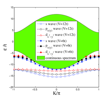
Figure 7: Dispersion relations of bound states along the line of $K_{x}=K_{y}=K$ for $V=6t$ and $V=12t$. As comparison, the particle-hole continuum is also shown (green shaded region).

III.2 Bound states in two dimension

Before presenting the numerical results, we discuss the symmetries of the effective Hamiltonian $H_{eff}$ in Eq. (7) in details. After a gauge transformation

$$|\vec{\rho}\rangle^{\prime}=|x,y\rangle^{\prime}=e^{-i(x\theta_{\hat{x}}+y\theta_{\hat{y}}})|x,y\rangle=e^{-i(x\theta_{\hat{x}}+y\theta_{\hat{y}}})|\vec{\rho}\rangle$$ (18)

with $\theta_{\hat{x}}\!\!=\!\!arctan(\frac{1}{3}tan(\frac{K_{x}}{2}))$ and $\theta_{\hat{y}}\!\!=\!\!arctan(\frac{1}{3}tan(\frac{K_{y}}{2}))$, we could remove the phase factors in the Hamiltonian and get

$$H_{eff}^{\prime} = H_{ph,0}^{\prime}+V_{ph}^{\prime},$$ (19)

$$H_{ph,0}^{\prime} = -t_{\hat{x}}\sum_{\vec{\rho},\vec{\sigma}_{x}}|\vec{\rho}\rangle^{\prime}\langle\vec{\rho}-\vec{\sigma}_{x}|^{\prime}-t_{\hat{y}}\sum_{\vec{\rho},\vec{\sigma}_{y}}|\vec{\rho}\rangle^{\prime}\langle\vec{\rho}-\vec{\sigma}_{y}|^{\prime},$$

$$V_{ph}^{\prime} = -V\sum_{\vec{\sigma}}|\vec{\sigma}\rangle^{\prime}\langle\vec{\sigma}|^{\prime}+t_{\hat{x}}\sum_{\vec{\sigma}_{x}}|\vec{\sigma}_{x}\rangle^{\prime}\langle 0|^{\prime}+h.c.$$

$$+t_{\hat{y}}\sum_{\vec{\sigma}_{y}}|\vec{\sigma}_{y}\rangle^{\prime}\langle 0|^{\prime}+h.c.,$$

where $\vec{\sigma}_{x}$ and $\vec{\sigma}_{y}$ denote the nearest neighbors along the $x$ and $y$ directions, respectively, and $t_{\hat{x}}\!\!\!\!=\!\!t\sqrt{9cos^{2}(\frac{K_{x}}{2})+sin^{2}(\frac{K_{x}}{2})}$ and $t_{\hat{y}}\!\!=t\sqrt{9cos^{2}(\frac{K_{y}}{2})+sin^{2}(\frac{K_{y}}{2})}$ are effective hoppings along the $x$ and $y$ directions.

When $K_{x}=\pm K_{y}$, $t_{\hat{x}}=t_{\hat{y}}$, $H_{eff}^{\prime}$ has symmetries of $D_{4}$ group. According to the irreducible representations of this group, the bound states can be classified and labeled with $s$, $p_{x(y)}$ and $d_{x^{2}-y^{2}}$ wave, respectively. Among them, the $s$ wave belongs to an identical representation $A_{1}$ of $D_{4}$ group, the degenerate $p_{x}$ and $p_{y}$ waves form a two dimensional irreducible representation $E$ of $D_{4}$ group, and the $d_{x^{2}-y^{2}}$ wave belongs to an irreducible representation $B_{1}$ of $D_{4}$ group.

When $K_{x}\neq\pm K_{y}$, $t_{\hat{x}}\neq t_{\hat{y}}$, the symmetry reduces to $D_{2}$, a subgroup of $D_{4}$. For simplicity, we still label the four bound states with $s$, $p_{x(y)}$ and $d_{x^{2}-y^{2}}$. Differently, here all the $s$ and $d$ wave belong to identical representations $A_{1}$ of $D_{2}$ group, while $p_{x}$($p_{y}$) wave belongs to an irreducible representation $B_{3}$($B_{2}$) of $D_{2}$ group. The degeneracy of $p_{x}$ and $p_{y}$ waves is lifted.

With $\rho^{\prime}=(0,0)$, $(\pm 1,\pm 1)$, Eq. $(9)$ reduces to five linear equations in two dimensional case. The free Green function $G_{0}(\vec{\rho},\vec{\rho}^{\prime})$ can be expressed with elliptic integrals Economou ; WORTIS . Although no brief solutions of $<\rho|G|\rho^{\prime}>$ could be found, we may factorize the particle-hole bound state equations and analyze the existence conditions for the bound states along the symmetric lines of $K_{x}=\pm K_{y}=K$ WORTIS . Considering the asymptotic behaviours of elliptic integrals, we get the thresholds of the interaction $V$ as follows: $V_{cr,s}(K)=t_{\hat{x}}$ for s wave, $V_{cr,p}(K)=\frac{2\pi}{2\pi-4}t_{\hat{x}}$ for $p_{x(y)}$ wave and $V_{cr,d}(K)=\frac{2\pi}{8-2\pi}t_{\hat{x}}$ for $d_{x^{2}-y^{2}}$ wave. From these thresholds, the existence region of every bound state is obtained respectively. For $s$ wave, we have

$$2arccos\sqrt{\frac{V^{2}-t^{2}}{8t^{2}}}\leq|K|\leq\pi,V\in(t,3t].$$

When $V>3t$, the $s$ wave bound state may be found in the whole Brillouin zone. The existence region of $p$ wave bound states is

$$2arccos\sqrt{\frac{(\frac{\pi-2}{\pi}V)^{2}-t^{2}}{8t^{2}}}\leq|K|\leq\pi,V\in(\frac{\pi}{\pi-2}t,\frac{3\pi}{\pi-2}t].$$

When $V>\frac{3\pi}{\pi-2}t$, the existence region extends to the whole Brillouin zone. For $d$ wave, existence region is expressed as

$$2arccos\sqrt{\frac{(\frac{4-\pi}{\pi}V)^{2}-t^{2}}{8t^{2}}}\leq|K|\leq\pi,V\in(\frac{\pi}{4-\pi}t,\frac{3\pi}{4-\pi}t].$$

When $V>\frac{3\pi}{4-\pi}t$, the d wave existence interval is the whole Brillouin zone.

Now we present the numerical results in two dimensions. At $\vec{K}=(0,0)$, four bound states could be found when $V\geq V_{cr,d}(0)=10.97t$. The wave functions with $s-$, $p_{x}-$ and $d_{x^{2}-y^{2}}-$wave symmetry for $V=12t$ are shown in Fig. 5. With the decrease of $V$, the highest $d_{x^{2}-y2}$-wave, the degenerate $p_{x(y)}$-waves and the lowest $s$-wave merge into the continuous spectrum one by one. Finally, all the bound states disappear when $V\leq V_{cr,s}(0)=3t$. In Fig. 6, we illustrate the variations of the bound state energies with the changes of $V$.

We then search for bound state solutions along the line of $K_{x}=K_{y}=K$. As shown in Fig. 7, there are four bound states for all $K\in[-\pi,\pi]$ at $V=12t$. At $V=6t$, $s$-wave exists in the whole region, while $p_{x(y)}$- and $d_{x^{2}-y^{2}}$-wave states appear at $0.52\pi<|K|\leq\pi$ and $0.69\pi<|K|\leq\pi$ respectively. Decreasing $V$ further, we find that the regions of the bound states shrink, and all the bound states disappear when $V<V_{cr,s}(\pm\pi)=1t$. Similar results are obtained along the line of $K_{x}=-K_{y}=K$.

Away from the lines of $K_{x}=\pm K_{y}$, the degeneracy of $p_{x}$ and $p_{y}$ bound states is lifted, as mentioned before. At a given $V$, different bound states have different existence regions in $\vec{K}$ space. Consequently, the number of bound states vary in the $(K_{x},K_{y})$ space. As an example, we show the number distribution of the bound states for $V=6t$ in Fig. 8.

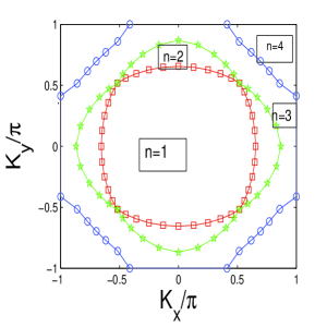
Figure 8: The number distribution of bound states in the first Brillouin zone at $V=6t$. As shown, there are more bound stats at the corners than that at the center in the first Brillouin zone.

III.3 Discussion of observations of the bound states

Inelastic light scattering directly measures the dynamical structure factor $S(\vec{q},\omega)$, the Fourier transformation of density correlations. Bragg spectroscopy has been proposed to detect quantum phases in optical lattice and successfully applied to measure the excitation spectra (phonons of BEC), the composition of the excitations and the Higgs-type amplitude mode in the superfluid condensate, as well as the particle-hole excitation energies in the Mott-insulator state Ye ; kurn ; Oosten ; Rey ; Ernst ; Bissbort ; Clement . When this technique is utilized in the study of ultra-cold polar molecules in the optical lattice, we may expect extra resonance peaks corresponding to the particle-hole bound states lying outside the particle-hole continuum.

Compared with the traditional solid state counterparts, the deep Mott insulating state with $t/U\ll 1$ and $zV<U$ can be realized by tuning the interaction parameters $t$, $U$ and $V$ in ultra-cold dipolar molecules in the optical lattices. In deep optical lattice the hopping is approximately evaluated as $t=(4/\sqrt{\pi})E_{r}(V_{opt}/E_{r})^{3/4}exp[-2(V_{opt}/E_{r})^{1/2}]$, with $V_{opt}=18\sim 20E_{r}$ the optical lattice depth and $E_{r}$ the lattice recoil energy Bloch . Under the condition of $\frac{as}{a_{\bot}}\ll 1$, where $a_{s}$ is the $s$-wave scattering length and $a_{\bot}=\sqrt{\frac{\hbar}{m\omega_{\bot}}}$ with $\omega_{\bot}$ transverse trapping frequency in one dimension or trapping frequency of the $z$ direction in two dimensions, the on-site interaction is estimated as $U_{1D}=\sqrt{\frac{2}{\pi}}\hbar\omega_{\bot}a_{s}/l_{0}$ and $U_{2D}=\frac{\sqrt{8\pi}\hbar^{2}a_{s}}{ma_{z}(2\pi)l_{0}^{2}}$ with $l_{0}=(\frac{E_{r}}{V_{opt}})^{\frac{1}{4}}\frac{a}{\pi}$ and $a$ the lattice constant Jaksch ; Bloch .

Taking Bose molecule $\mathrm{{{}^{23}Na^{7}Li}}$ for example, we may estimate the typical values of $t$, $U$ and $V$ for observing the particle-hole bound state. The molecule prepared in the ground state has a permanent electric moment $d=0.58D$ Mabrouk . With a lattice constant $a\sim 0.5\mu m$, $a_{s}/a\sim 0.01$ and the transversal tapping frequency $\omega_{\bot}\sim 2\pi\times 10^{4}\mathrm{Hz}$, we have $t\sim 1nK$, $U_{1D}\sim 25nK$ and $U_{2D}\sim 50nK$. The nearest-neighbor interaction $V$ can be tuned as $V\sim 10nK$ with an applied electric field.

IV Summary

In summary, we have investigated bound states of particle-hole pair resulting from the dipole-dipole interaction between polar molecules in the optical lattice. For a large enough dipole-dipole interaction, two degenerate bound states, which correspond to a particle on the left and the right of a hole, are shown to exist in one dimension. While in two-dimensional case, four bound states, with $s$-, $p_{x(y)}$- and $d_{x^{2}-y^{2}}$- symmetry respectively, are found along the lines of $K_{x}=\pm K_{y}$. Away from the lines of $K_{x}=\pm K_{y}$, the degeneracy between $p_{x}$ and $p_{y}$ waves is lifted. With decreasing the nearest-neighbor interaction $V$, the energies of the bound states increase and merge into the particle-hole continuum gradually. The wave functions, the dispersion relations and the existence regions of the bound states are studied in details. For a given nearest-neighbor $V$, the number of bound states is different in different regions of $\vec{K}$ space and a number distribution of bound states is given for the nearest-neighbor $V=6t$ in two dimensions. The possible experimental observation of the particle-hole bound states is also discussed.

Electron-hole bound state excitations (excitons) have been extensively studied for many years and very recently, the excitonic Bose-Einstein condensates have been realized experimentally in semiconductors butov ; kasprzak . We hope our study on the particle-hole bound states in bosonic systems would enrich our understanding of elementary excitations in quantum many-body systems and stimulate more efforts on the bound state phenomena in various systems such as magnets, superconductors and atomic systems.

Acknowledgements: This work was supported by the NKBRSFC under grants Nos. 2011CB921502, 2012CB821305, 2009CB930701, 2010CB922904, NSFC under grants Nos. 10934010, 60978019 and NSFC-RGC under grants Nos. 11061160490 and N-HKU748/10.

References

- (1) For reviews, see L. D. Carr, D. DeMille, R. V. Krems and J. Ye, New J. Phys. 11, 055049 (2009); O. Dulieu and C. Gabbanini, Rep. Prog. Phys. 72, 086401 (2009).
- (2) S. Jochim, M. Bartenstein, A. Altmeyer, G. Hendl, S. Riedl, C. Chin, J. H. Denschlag, R. Grimm, Science 302, 2101 (2003).
- (3) M. Greiner, C. A. Regal and D. S. Jin, Nature 426, 537 (2003).
- (4) T. Volz, N. Syassen, D. M. Bauer, E. Hansis, S. Dürr and G. Rempe, Nature Physics 2, 692 (2006).
- (5) J. G. Danzl, M. J. Mark, E. Haller, M. Gustavsson, R. Hart, J. Aldegunde, J. M. Hutson and H.-C. Nägerl, Nature Physics 6, 265 (2010).
- (6) K. K. Ni, S. Ospelkaus, M. H. G. de Miranda, A. Pe’er, B. Neyenhuis, J. J. Zirbel, S. Kotochigova, P. S. Julienne, D. S. Jin, J. Ye, Science 322, 231 (2008).
- (7) S. Ospelkaus, A. Pe’er, K. K. Ni, J. J. Zirbel, B. Neyenhuis, S. Kotochigova, P. S. Julienne, J. Ye and D. S. Jin, Nature Physics 4, 622 (2008).
- (8) J. M. Sage, S. Sainis, T. Bergeman and D. DeMille, Phys. Rev. Lett. 94, 203001 (2005).
- (9) D. Wang, J. T. Kim, C. Ashbaugh, E. E. Eyler, P. L. Gould and W. C. Stwalley, Phys. Rev. A 75, 032511 (2007).
- (10) B. C. Sawyer, B. L. Lev, E. R. Hudson, B. K. Stuhl, M. Lara, J. L. Bohn and J. Ye, Phys. Rev. Lett. 98, 253002 (2007).
- (11) D. DeMille, Phys. Rev. Lett. 88, 067901 (2002).
- (12) H. P. Büchler, E. Demler, M. Lukin, A. Micheli, N. Prokof’ev, G. Pupillo, and P. Zoller, Phys. Rev. Lett. 98, 060404 (2007).
- (13) L. Santos, G.V. Shlyapnikov, P. Zoller and M. Lewenstein, Phys. Rev. Lett. 85, 1791 (2000).
- (14) N. R. Cooper, E. H. Rezayi and S. H. Simon, Phys. Rev. Lett. 95, 200402 (2005).
- (15) M. A. Baranov, Klaus Osterloh and M. Lewenstein, Phys. Rev. Lett. 94, 070404 (2005).
- (16) K. Góral, L. Santos and M. Lewenstein, Phys. Rev. Lett. 88, 170406 (2002).
- (17) C. Menotti, C. Trefzger and M. Lewenstein, Phys. Rev. Lett. 98, 235301 (2007).
- (18) C. Lin, E. Zhao, and W. V. Liu, Phys. Rev. B 81, 045115 (2010).
- (19) C. Bruder, R. Fazio, and G. Schön, Phys. Rev. B 47, 342 (1993).
- (20) A. van Otterlo, K. H. Wagenblast, R. Baltin, C. Bruder, R. Fazio and G. Schön, Phys. Rev. B 52, 16176 (1995).
- (21) P. Niyaz, R. T. Scalettar, C. Y. Fong and G. G. Batrouni, Phys. Rev. B 50, 362 (1994).
- (22) P. Sengupta, L. P. Pryadko, F. Alet, M. Troyer, and G. Schmid, Phys. Rev. Lett. 94, 207202 (2005).
- (23) S. R. Hassan, L. de Medici, and A.-M. S. Tremblay, Phys. Rev. B 76, 144420 (2007).
- (24) M. Iskin and J. K. Freericks, Phys. Rev. A 79, 053634 (2009).
- (25) R. V. Pai and R. Pandit, Phys. Rev. B 71 104508 (2005).
- (26) Y. C. Chen, R. G. Melko, S. Wessel, and Y. J. Kao, Phys. Rev. B 77, 014524 (2008).
- (27) M. P. A. Fisher, P. B. Weichman, G. Grinstein, D. S. Fisher, Phys. Rev. B 40, 546 (1989).
- (28) D. van Oosten, P. vanderStraten, and H. T. C. Stoof, Phys. Rev. A 63, 053601 (2001).
- (29) D. L. Kovrizhin, G. V. Pai, and S. Sinha, Europhys. Lett. 72, 162 (2005).
- (30) F. B. Gallagher and S. Mazumdar, Phys. Rev. B 56, 15025 (1997); W. Barford, Phys. Rev. B 65, 205118 (2002); K. A. Al-Hassanieh, F. A. Reboredo, A. E. Feiguin, I. González, and E. Dagotto, Phys. Rev. Lett. 100, 166403 (2008).
- (31) D. C. Mattis, The Theory of Magnetism, Vol. I: Statics and Dynamics, Springer-Verlag Series in Solid State Sciences (Berlin-New York, 1981).
- (32) E. N. Economou, Green’s Functions in Quantum Physics, Third Edition, Springer-Verlag Series in Solid State Sciences (Berlin, 2006).
- (33) N. Nygaard, R. Piil, and K. Mølmer, Phys. Rev. A 78, 023617 (2008).
- (34) W. Barford, Phys. Rev. B 65, 205118 (2002).
- (35) M. Wortis, Phys. Rev. 132, 85 (1963).
- (36) J. W. Ye, J. M. Zhang, W. M. Liu, K. Y. Zhang, Y. Li, and W. P. Zhang, Phys. Rev. A 83, 051604(R) (2011).
- (37) D. M. Stamper-Kurn, A. P. Chikkatur, A. Görlitz, S. Inouye, S. Gupta, D. E. Pritchard, and W. Ketterle, Phys. Rev. Lett. 83, 2876 (1999).
- (38) D. van Oosten, D. B. M. Dickerscheid, B. Farid, P. vanderStraten, and H. T. C. Stoof, Phys. Rev. A 71, 021601 (2005).
- (39) A. M. Rey, P. B. Blakie, G. Pupillo, C. J. Williams, and C. W. Clark, Phys. Rev. A 72, 023407 (2005).
- (40) P. T. Ernst, S. Götze, J. S. Krauser, K. Pyka, D.-S. Lühmann, D. Pfannkuche, and K. Sengstock, Nature Physics 6, 56 (2010).
- (41) U. Bissbort, S. Götze, Y. Li, J. Heinze, J. S. Krauser, M. Weinberg, C. Becker, K. Sengstock, and W. Hofstetter, Phys. Rev. Lett. 106, 205303 (2011).
- (42) D. Clément, N. Fabbri, L. Fallani, C. Fort, and M. Inguscio, Phys. Rev. Lett. 102, 155301 (2009).
- (43) I. Bloch, J. Dalibard, and W. Zwerger, Rev. Mod. Phys. 80, 885 (2008).
- (44) D. Jaksch, C. Bruder, J. I. Cirac, C. W. Gardiner, and P. Zoller, Phys. Rev. Lett. 81, 3108 (1998).
- (45) N. Mabrouk and H. Berriche, J. Phys. B: At. Mol. Opt. Phys. 41, 155101 (2008).
- (46) L. V. Butov, C. W. Lai, A. L. Ivanov, A. C. Gossard, and D. S. Chemla, Nature 417, 47 (2002).
- (47) J. Kasprzak, M. Richard, S. Kundermann, A. Baas, P. Jeambrun, J. M. J. Keeling, F. M. Marchetti, M. H. Szymańska, R. André, J. L. Staehli, V. Savona, P. B. Littlewood, B. Deveaud, and L. S. Dang, Nature 443, 409 (2006).