Regular and irregular geodesics on spherical harmonic surfaces

Abstract

The behavior of geodesic curves on even seemingly simple surfaces can be surprisingly complex. In this paper we use the Hamiltonian formulation of the geodesic equations to analyze their integrability properties. In particular, we examine the behavior of geodesics on surfaces defined by the spherical harmonics. Using the Morales-Ramis theorem and Kovacic algorithm we are able to prove that the geodesic equations on all surfaces defined by the sectoral harmonics are not integrable, and we use Poincaré sections to demonstrate the breakdown of regular motion.

1 Introduction

The study of the qualitative behavior of geodesics goes back to the beginnings of differential geometry; in fact Clairault’s relation dates from the 1740’s. One of the many interesting features of the geodesic equations is their complexity: how can we solve such difficult nonlinear differential equations, and indeed what does it mean to ‘solve’ a differential equation at all? In the general development of Lagrangian/Hamiltonian dynamics the issue of integrability came to the fore, and the use of first integrals to solve a dynamical system via quadratures was developed. By integrability here we mean intebrability in the sense of Louiville: a Hamiltonian system with $n$ degrees of freedom is Louiville integrable if there exist $n$ independent first integrals of the motion in involution (vanishing pairwise Poisson brackets). This formalism in turn lead to the consequences of non-integrability, the onset of chaos and the celebrated KAM theory. For a particularly interesting introduction to this topic see Berry [5], McCauley [22] or José and Saletan [17].

The integrability of the geodesic equations on some surfaces, and therefore the regularity of the geodesic trajectories, has been well understood for many years. Clairault’s relation [10] provides a second integral for surfaces of revolution, and Jacobi [18] integrated the triaxial ellipsoid. These results have been extended to $n$-dimensional ellipsoids and to quadrics in general (see Audin [2]), where interestingly degenerate cases can prove more difficult to analyse (see Davison et al [12]). Recently, the integrability of the geodesic equations has been demonstrated for more abstract manifolds, defined in terms of Lie groups (see for example Thimm [31]). Aside from being interesting in their own right, the geodesics of a manifold also have some useful applications. For example, Maupertius’s principle [7] relates the dynamics on an isoenergetic level of any mechanical system to the geodesics of a manifold, and the relativistic formulation of gravity dictates that massive particles move along the timelike geodesics of spacetime [33].

There are many powerful results regarding the non-integrability of the geodesic flow on manifolds of a certain class, for example a theorem of Kolokol’tsov [19] says that two-dimensional compact surfaces of genus $g>1$ do not admit geodesic flows that are integrable with a second integral polynomial with respect to the momenta (see Bolsinov [6] for a review and references). What’s more the integrable geodesic flows on surfaces with $g=0,1$ with second integrals either linear or quadratic in the momenta are completely described. Nonetheless, new examples of integrable geodesic flows with second integrals cubic in the momenta have recently been found (see for example Dullin and Matveev [13]) and the possibility of non-polynomial, and in particular meromorphic second integrals, is open.

A very significant recent development with regards integrability has been the theorem of Morales Ruiz and Ramis [28, 29]. This theorem provides a link between the question of whether a nonlinear Hamiltonian system is integrable (with meromorphic first integrals) with whether the variational equations of a non-trivial solution to the Hamiltonian system are solvable. This is a great advance as the variational equations are linear with variable coefficients, and the solvability of equations of this type may be addressed using differential Galois theory. This approach has proved very successful (we give here only some examples): in Morales Ruiz and Ramis [29] the authors use this formalism to prove the non-integrability of certain problems from mechanics and celestial mechanics; in Morales Ruiz et al [30] the non integrability of Hill’s problem is shown; in Pujol et al [27] the non-integrability of the swinging Atwood’s machine is demonstrated; in Acosta-Humánez et al [1] some problems in celestial mechanics are studied and in Bardin et al [4] the generalized Jacobi problem is studied. In the majority of these papers, the solvability of the variational equations is determined using Kovacic’s algorithm, and this is the approach we will follow in this work, with a description of the algorithm and relevant references given in Section 4.

To the best of our knowledge this powerful Morales-Ramis formalism has not been applied to the study of geodesics on manifolds and their integrability properties, and the approach taken in this work is novel in this respect. In the following we will examine the properties of geodesics on surfaces defined in terms of the spherical harmonics, and we shall rigorously prove using the Morales-Ramis theorem the non-integrability of the geodesic equations on surfaces defined in terms of sectoral spherical harmonics. Thus we present a two-parameter family of surfaces which appear very simple and symmetrical and yet have complex and indeed chaotic geodesic curves on them; this is a novel addition as the surfaces for which non-integrability of the geodesic flow has been rigorously proved is small. Finally, we will also use Poincaré sections to display the breakdown of regular motion as well as to understand the various families of closed geodesics on the surfaces; again this approach is novel in the case of geodesic flows.

The layout of the paper shall be as follows: In Section 2 we review the formulation of the geodesic equations and describe the classes of surfaces which will be examined. In Section 3 we use Poincaré sections to exhibit the breakdown in regular motion suggesting non-integrability, as well as describe the main families of closed geodesics on the surface. Finally in Section 4 we will review some necessary theory and prove the main result: the non-integrability of the geodesic equations on sectoral harmonic surfaces with $n>1$.

2 The geodesic equations

One geometrical description of a geodesic curve is as follows: of all the curves connecting two nearby points on a manifold, the one that extremizes the length along that curve is the geodesic (minimizes in the case of a positive definite manifold). An alternative dynamical description is to imagine a test particle moving in the manifold free from external forces; if the particle’s speed is constant, then the path it follows is a geodesic. Consequently, we may define a (dynamic) Lagrangian $\mathcal{L}$ in the following way: let the coordinates $x^{a}$ parameterize the $n$-dimensional manifold $(\mathcal{M},\mbox{\boldmath$g$})$ and let $s$ parameterize a curve in the manifold, such that $x^{a}=x^{a}(s)$. The length of the tangent vector to this curve is

$$\left(\sum_{a,b=1}^{n}g_{ab}\ \dot{x}^{a}\,\dot{x}^{b}\right)^{1/2},$$

but this is simply the speed. Here $g_{ab}$ are the components of the metric tensor in the $x^{a}$ coordinate system, and from now on a dot denotes differentiation w.r.t. $s$ and summation over repeated indices is implied. We may define the kinetic energy as one half the square of this quantity (assuming unit mass), and therefore the Lagrangian function is

$$\mathcal{L}=\tfrac{1}{2}\ g_{ab}\ \dot{x}^{a}\,\dot{x}^{b}.$$ (1)

Putting the Lagrangian function into the Euler-Lagrange equations we arrive at the geodesic equations,

$$\frac{d^{2}x^{a}}{ds^{2}}+\Gamma^{a}_{bc}\ \frac{dx^{b}}{ds}\frac{dx^{c}}{ds}=0,$$ (2)

where the Christoffel symbols (metric connections) are given by

$$\Gamma^{a}_{bc}=\tfrac{1}{2}g^{ad}(g_{bd,c}+g_{cd,b}-g_{bc,d}).$$ (3)

The equivalent Hamiltonian formulation is clear, by simply letting $\mathcal{H}=\mathcal{L}$. For a more detailed derivation of the geodesic equations see Paternain [25], Do Carmo [10] or alternatively Wald [33]. We note that some authors prefer to use the coordinates of the space the manifold is embedded in, and place a constraint on these coordinates (see for example Davison et al [12]). This approach does not suit our purposes here.

2.1 Surfaces defined in polar form

Let us consider two-dimensional surfaces given in polar form, that is

$$r=r(\theta,\phi),$$ (4)

where $(\theta,\phi)$ are the standard spherical coordinates with $0<\theta<\pi,\ 0<\phi<2\pi$. We may calculate the geodesic equations in the following way: the line element for $\mathbb{R}^{3}$ in spherical coordinates is given by

$$ds^{2}=dr^{2}+r^{2}d\theta^{2}+r^{2}\sin^{2}\theta d\phi^{2}.$$

On the surface we have $r=r(\theta,\phi)$ and hence $dr=r_{,\theta}d\theta+r_{,\phi}d\phi$ and so

$$ds^{2}=(r_{,\theta}^{2}+r^{2})d\theta^{2}+2r_{,\theta}r_{,\phi}d\theta d\phi+(r_{,\phi}^{2}+r^{2}\sin^{2}\theta)d\phi^{2},$$ (5)

from which the metric coefficients may be read off, inserted into the Christoffel symbols in (3) which in turn are put into the geodesic equations in (2), namely

$$\ddot{\theta}+\Gamma^{\theta}_{\theta\theta}\dot{\theta}^{2}+2\Gamma^{\theta}_{\theta\phi}\dot{\theta}\dot{\phi}+\Gamma^{\theta}_{\phi\phi}\dot{\phi}^{2}=0,$$ (6)

$$\ddot{\phi}+\Gamma^{\phi}_{\theta\theta}\dot{\theta}^{2}+2\Gamma^{\phi}_{\theta\phi}\dot{\theta}\dot{\phi}+\Gamma^{\phi}_{\phi\phi}\dot{\phi}^{2}=0.$$ (7)

It will be most informative for later analysis to describe closed geodesics on these surfaces. For this, we note the following: if a smooth surface has a plane of symmetry, then the curve formed by the intersection of the plane of symmetry with the surface will be a geodesic. Geometrically the reason for this is clear: if the surface is smooth the plane of symmetry will be normal to the surface, and any normal curve is geodesic. For the sake of the analysis to follow however we will make the following argument: let us arrange the coordinate system so that the plane of symmetry is given by $\theta=\pi/2$; on this plane $r_{,\theta}=0$. From (6), we see $\theta=\pi/2,\dot{\theta}=0$ will be a solution if $\Gamma^{\theta}_{\phi\phi}(\theta=\pi/2)=0$. Direct calculation from (3) and (5) gives

$$\Gamma^{\theta}_{\phi\phi}=\frac{r_{,\theta}(rr_{,\phi\phi}\sin^{2}\theta-2r_{,\phi}^{2}\sin^{2}\theta-r^{2}\sin^{4}\theta)-\cos\theta(r^{3}\sin^{3}\theta+rr_{,\phi}^{2}\sin\theta)}{r(r^{2}\sin^{2}\theta+r_{,\theta}^{2}\sin^{2}\theta+r_{,\phi}^{2})},$$

which vanishes on $\theta=\pi/2$. This is equivalent to the ‘invariant plane’ construction typical in dynamics which we will describe more of below; we will subsequently refer to such geodesics as planar geodesics.
Of course, to describe the geodesic completely we must solve the geodesic equations reduced to this plane, namely $\ddot{\phi}+\Gamma^{\phi}_{\phi\phi}(\theta=\pi/2)\dot{\phi}^{2}=0$; we will address this issue in Section 4.

2.2 Surfaces defined by the spherical harmonics

The surfaces we will examine in this work are those defined by the spherical harmonics in the following polar form

$$r(\theta,\phi)=1+\varepsilon\,Y_{lm}(\theta,\phi).$$ (8)

Here $\varepsilon$ is a small parameter and $Y_{lm}$ is the spherical harmonic of degree $l$ and order $m$ (see Wang and Guo [34]) given by

$$Y_{lm}(\theta,\phi)=\sqrt{\frac{(2l+1)(l-m)!}{4\pi(l+m)!}}\ P^{m}_{l}(\cos\theta)e^{im\phi},\quad m=0,\pm 1,\ldots,\pm l,$$

where $P^{m}_{l}$ are the associated Legendre polynomials. We may absorb the orthonormality coefficient into $\varepsilon$ and take the real part of the exponential to write

$$r(\theta,\phi)=1+\varepsilon\,P^{m}_{l}(\cos\theta)\cos(m\phi),\quad 0\leq\varepsilon<1.$$ (9)

With a slight abuse of language, we shall refer to surfaces defined in terms of the spherical harmonic functions as ‘spherical harmonic surfaces’ and so on. We chose to study these surfaces for the following reasons:

1. The spherical harmonics are complete, that is any function continuous over the sphere may be decomposed into a (possibly infinite) set of spherical harmonics. As such, general surfaces of a certain class can be decomposed into a number of spherical harmonic surfaces.

2. The spherical harmonics naturally have the smoothness and regularity required for this analysis, and are non-singular as long as $\varepsilon<1$.

3. The small parameter allows for a perturbative approach: with $\varepsilon=0$ the surface is a sphere, and as we let $\varepsilon$ grow we are deforming the surface away from the sphere.

4. The spherical harmonic surfaces are compact, enabling the Poincaré section analysis of the next section.

There are three classes of spherical harmonic: the zonal, the sectoral and the tesseral (see Figure 1 for representative examples).

Zonal

These are the spherical harmonics with $m=0$, and thus $r=1+\varepsilon\,P_{l}^{0}(\cos\theta)$. Since $r_{,\phi}=0$, this means $\partial\mathcal{L}/\partial\phi=0$, which from the Euler- Lagrange equations leads to $\partial\mathcal{L}/\partial\dot{\phi}=$constant. This is of course Clairault’s integral, as the zonal harmonic surfaces are surfaces of revolution; the motion of the geodesics on zonal harmonic surfaces will therefore be regular.

Sectoral

These are the spherical harmonics for which $l=m$. We shall relabel the degree/order $n$ in this case, and $Y^{n}_{n}$ takes on a simple form: the sectoral harmonic surfaces are defined by

$$r=1+\varepsilon\,\sin^{n}(\theta)\cos(n\phi).$$ (10)

This describes a two-parameter family of surfaces which admit planes of symmetry; as such they provide an interesting case for analysis and will form the main part of this work.

Tesseral

These are the remaining members of the family, with $m=\pm 1,\ldots$,$\pm l-1$. We will not examine these surfaces in any detail in this work, but discuss them briefly in the conclusions.

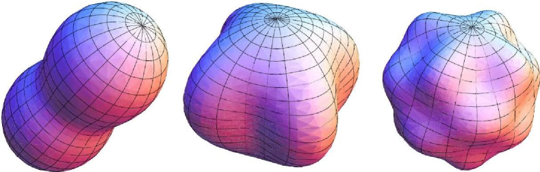
Figure 1: Examples of spherical harmonic surfaces, for various values of $\varepsilon$: on the left the $l=2,m=0$ zonal harmonic, in the centre the $l=m=4$ sectoral harmonic, and on the right the $l=7,m=4$ tesseral harmonic.

The Hamiltonian function for the geodesic equations on the sectoral harmonic surfaces is given by

$$2\mathcal{H}=g_{\theta\theta}\dot{\theta}^{2}+2g_{\theta\phi}\dot{\theta}\dot{\phi}+g_{\phi\phi}\dot{\phi}^{2}$$ (11)

where

$$g_{\theta\theta}=(1+\varepsilon\cos(n\phi)\sin^{n}(\theta))^{2}+\varepsilon^{2}n^{2}\cos^{2}(n\phi)\sin^{2n-2}(\theta),$$

$$g_{\theta\phi}=g_{\phi\theta}=-\varepsilon^{2}n^{2}\cos(n\phi)\sin(n\phi)\cos(\theta)\sin^{2n-1}(\theta),$$

$$g_{\phi\phi}=\sin^{2}(\theta)(1+\varepsilon\cos(n\phi)\sin^{n}(\theta))^{2}+\varepsilon^{2}n^{2}\sin^{2}(n\phi)\sin^{2n}(\theta).$$

It is clear from (10), or indeed Figure 1, that the $n$th sectoral harmonic surface has $n+1$ planes of symmetry: $n$ vertical/meridianal planes given by $\phi=\pi i/n,\ i=0,\ldots,n-1$ and 1 horizontal plane given by $\theta=\pi/2$, the equator. Each of these planes defines a planar geodesic as described above.

3 Poincaré Sections

This is a much used technique to attempt to visualize the whole of phase space in the case of a 2-degree of freedom Hamiltonian system. By fixing a value of $\mathcal{H}=\mathcal{H}_{0}$, a 3-dimensional submanifold of phasespace, and intersecting this manifold with a hyperplane (typically given by a coordinate taking on a fixed value), we consider successive intersections of solution trajectories with this hyperplane. If the Hamiltonian system is integrable, then the second integral restricts the solutions further to a 2-dimensional submanifold of phasespace, whose intersections with the hyperplane will trace out a closed curve. On the other hand, if the Hamiltonian system is not integrable then successive intersections of the solution trajectory with the hyperplane may instead fill a 2-dimensional region.

Typically, for a fixed set of parameters a number of Poincaré sections for various values of the ‘energy’ $\mathcal{H}_{0}$ must be drawn, for example in the Hénon-Heiles system [16]. This is not necessary in the current situation, since the numerical value of the Hamiltonian function may be changed from $\mathcal{H}_{0}$ to $\mathcal{H}_{1}$ by the change of independent variable $s\to\sqrt{\mathcal{H}_{0}/\mathcal{H}_{1}}\,s$. Therefore the numerical value of $\mathcal{H}$ signifies the parameterization of the geodesic curve, rather than any ‘energy’ concept. Indeed, any affine coordinate transformation $s\to\alpha s+\beta$ will change the value of $\mathcal{H}$ but leaves (2) invariant. Therefore, any qualitative change in the Poincaré sections will be due to variations in the surface’s parameters ($n$ and $\varepsilon$ for the sectoral harmonic surfaces), rather than the value of $\mathcal{H}$. In what follows, we will assume the geodesic is parameterized by arc-length (sometimes referred to as ‘unit-speed curves’ in the literature), and therefore

$$\mathcal{H}\equiv\tfrac{1}{2}.$$

In choosing the hyperplane to act as the Poincaré section we must ensure all solutions intersect the hyperplane transversally; no tangential grazings are allowed, and a guarantee that the trajectory will intersect the surface again is preferable. Any of the $n+1$ planes of symmetry would be suitable candidates, although for simplicity we will use the equatorial plane (some comments regarding the use of meridianal planes are given in Appendix A). First we prove the following lemma:

Lemma 1.

Along a geodesic, $\theta$ cannot obtain a maximum/minimum in the northern/southern hemisphere respectively, at least for moderate values of $\varepsilon$.

Proof.

We remind the reader that $\theta$ is measured down from the positive $z$-axis, and the northern and southern hemispheres are given by $\theta\in(0,\pi/2)$ or $(\pi/2,\pi)$ respectively. Due to symmetry, we need only show that $\theta$ cannot obtain a maximum for $\theta\in(0,\pi/2)$.
From (6), a maximum w.r.t. $\theta$ in the northern hemisphere would require $\Gamma^{\theta}_{\phi\phi}>0$ for some $\theta\in(0,\pi/2)$ (on the sphere, $\Gamma^{\theta}_{\phi\phi}=-\cos\theta\sin\theta<0$ for $0<\theta<\pi/2$, ruling out this possibility). We can write

$$\Gamma^{\theta}_{\phi\phi}=-\frac{r\cos\theta\sin^{3}\theta}{det(g)}\ f(\sin\theta,\cos(n\phi);n,\varepsilon).$$

As the surface is positive definite to prove the lemma we must show $f\geq 0$ in $\Omega=\{0<\theta<\pi/2$, $0<\phi<2\pi\}$. Letting $\rho=\sin\theta$ with $0<\rho<1$ in $\Omega$, we can write

$$f(\rho)=1+a_{1}\rho^{n}+a_{2}\rho^{2n-2}+a_{3}\rho^{2n}+a_{4}\rho^{3n-2}+a_{5}\rho^{3n}$$

where the $a_{i}$ depend on $\cos(n\phi),\ n$ and $\varepsilon$ ($\phi$ here being the coordinate at which the proposed maximum takes place). When $\cos(n\phi)>0$, all the $a_{i}$ are positive and so $f(\rho)>0$ in $\Omega$.
If, on the other hand, $\phi$ is such that $\cos(n\phi)<0$, Descarte’s rule of signs tells us that $f(\rho)$ can only have 1 or 3 roots in $0<\rho<1$, and since $f(0)>0$ this is impossible unless $f(1)<0$. Letting $f(1)=0$ gives a cubic in $\cos(n\phi)$, and we can then find explicitly the value of $\varepsilon$ as a function of $n$ at which the value of $f(1)$ becomes negative for some values of $\phi$. If we call this critical value $\varepsilon^{*}$, then for example when $n=2,3,4$ we find $\varepsilon^{*}=0.57,0.497,0.445$. ∎

Note this lemma rules out the possibility of closed geodesics which do not intersect the equator at some stage (the only $\theta=$ constant geodesic is the equator). What it does not rule out, however, is the possibility of a geodesic asymptotically approaching the equator. In fact, this cannot occur as the equator is of elliptic type. A rigorous proof of the non-hyperbolic nature of the equator is too much of a digression; certainly numerical evidence can be easily provided using Floquet theory (see [35] for a detailed description) by calculating the eigenvalues of the monodromy matrix and showing they remain on the unit circle in the complex plane for moderate values of $\varepsilon>0$ and various values of $n$. Having said that the most immediate demonstration of the elliptic nature of the equator is to be found in the Poincaré section shown in Fig. A.3.

Proposition 1.

With the equatorial geodesic of elliptic type, any geodesic which intersects the equatorial plane transversally must re-intersect the equatorial plane an infinite number of times, at least for moderate values of $\varepsilon$.

Proof.

First we can see that any trajectory which intersects the equatorial plane transversally cannot subsequently graze this plane tangentially as it is an invariant plane. If we consider a geodesic which crosses the equator with $\dot{\theta}<0$ (i.e. entering the northern hemisphere) then there are two possibilities: 1) the geodesic does not pass through the north pole, and 2) the geodesic passes through the north pole. In the event of case 1), the geodesic must attain a minimum w.r.t. $\theta$ ($\theta$ is an initially positive decreasing continuous function of arc-length and so must either: attain a minimum; pass through zero (case 2); or asymptote to some constant value which is impossible as the surface is compact and there are no equilibrium points or closed geodesics contained in a hemisphere). As the geodesic cannot attain a maximum w.r.t. $\theta$ in the northern hemisphere or asymptote to the equator, it must subsequently re-intersect the equator. In the event of case 2), consider a geodesic which starts at the north pole. While there is a degeneracy in defining $\phi$ at the poles there is no problem in defining $\dot{\phi}$. Following the geodesic in this direction it must intersect the equator for the reasons given in case 1), but the same can be said if we follow the geodesic “backwards”, and so it must intersect the equator in both directions. ∎

A final consideration is the ranges of velocities the geodesics may explore. On any of the planes of symmetry, either $r_{,\theta}$ or $r_{,\phi}$ vanishes, thus (from (5)) $g_{\theta\phi}=0$. Therefore on the section we have

$$g_{\theta\theta}\dot{\theta}^{2}+g_{\phi\phi}\dot{\phi}^{2}=1,$$ (12)

which is an ellipse of semi-axes $1/\sqrt{g_{\theta\theta\phantom{\phi}}}$ and $1/\sqrt{g_{\phi\phi}}$. Since $g_{\phi\phi}(\theta=\pi/2)=(1+\varepsilon\cos(n\phi))^{2}+\varepsilon^{2}n^{2}\sin^{2}(n\phi)$, when choosing our initial conditions to generate the Poincaré section plots we should therefore choose random values for $\dot{\phi}$ in the range $\dot{\phi}\in(-\dot{\phi}_{m},\dot{\phi}_{m})$ with

$$\dot{\phi}_{m}=\left\{\begin{array}[]{cc}\frac{1}{1+\varepsilon}&\quad\textrm{if}\ \varepsilon<\frac{1}{n^{2}-1}\\ \\ \frac{1}{\sqrt{\frac{n^{2}(1+\varepsilon^{2}(n^{2}-1))}{(n^{2}-1)}}}&\quad\textrm{if}\ \varepsilon>\frac{1}{n^{2}-1}.\end{array}\right.$$ (13)

The initial conditions can now be chosen in the following way: random values for $\phi$ are chosen in the range $(0,2\pi)$, random values for $\dot{\phi}$ in the range $(-\dot{\phi}_{m},\dot{\phi}_{m})$, and the value of $\dot{\theta}$ is found from $\mathcal{H}=\tfrac{1}{2}$ (we will always take the positive value to give a ‘downward’ pointing geodesic). The geodesic with these initial conditions is followed for a long time and intersections with the equatorial plane with $\dot{\theta}>0$ are monitored. We show in Figure 2 some of the resulting Poincaré sections for the case of the $n=3$ sectoral harmonic surface. Some interesting points to note are:

1. There are three main families of closed geodesics; these appear as fixed points of the Poincaré section, and are as follows: Firstly there are $n$ planar geodesics as described in Section 2 leading to fixed points at $\phi=\pi i/n,i=1,\ldots,n$ and $\dot{\phi}=0$. Secondly on the sectoral surfaces with $n$ odd there are $n$ perpendicular geodesics, which are not planar but intersect the equator at right angles, leading to fixed points roughly midway between those due to the planar geodesics. Thirdly there are oblique geodesics which are simple (period-1) and give rise to fixed points off the horizontal axis of the Poincaré section.
   Of course, there are an infinite number of closed geodesics on topological spheres (see Bangert [3] and Franks [15]) and we make no attempt to classify them all.

2. The stability of these closed geodesics is perhaps not what would be expected (Note: we are using only the Poincaré sections to draw conclusions about stability; a more rigorous stability analysis would make an interesting topic for future research). Consider first the sectoral surfaces with $n$ even, as shown in Figure 1 (b). The planar geodesics alternate between those for which $\partial^{2}r/\partial\phi^{2}\leq 0$ and those for which $\partial^{2}r/\partial\phi^{2}\geq 0$ everywhere along the curve. In analogy with the surfaces of revolution [10], we might therefore expect that these geodesics would alternate between stability and instability, respectively. However this is not the case: all planar geodesics are in fact stable, leading to elliptic fixed points on the Poincaré section.
   If we now consider the sectoral surfaces for $n$ odd, then $\partial^{2}r/\partial\phi^{2}$ is both positive and negative along each planar geodesic. In fact, these planar geodesics are all unstable; what’s more each is homoclinic to itself (at least for small $\varepsilon$, see below) and thus admits two elliptic points within its homoclinic loops, see Figure 2. These elliptic points form a fourth family of closed geodesics, and some numerical experimentation reveals these are also period-1.
   The perpendicular geodesics mentioned in 1. are all stable, leading to elliptic fixed points in the Poincaré section, and most importantly the oblique geodesics are unstable, leading to hyperbolic fixed points. These hyperbolic fixed points are heteroclinic to one another as Figure 2 shows (in fact there are complex heteroclinic networks, where up to $2n$ saddles are connected to one another), and this is the crucial ingredient leading to chaotic motion, which we shall describe next.

3. As is clear from Figure 2, chaotic motion takes place for large $\varepsilon$, that is as we deform the surface away from the sphere. The onset of chaos as depicted in Figure 2 is straight out of a textbook: the invariant manifolds of unstable fixed points intersect leading to a heteroclinic tangle, and as $\varepsilon$ increases further rational invariant tori are destroyed. This phenomenon is well described in the literature, see for example José and Saletan [17], Calkin [9] or Berry [5]. The value of $\varepsilon$ at which this onset of chaotic motion takes place varies for different values of $n$, but note that we see chaotic motion for values of $\varepsilon$ less than those mentioned in Lemma 1.

(a)
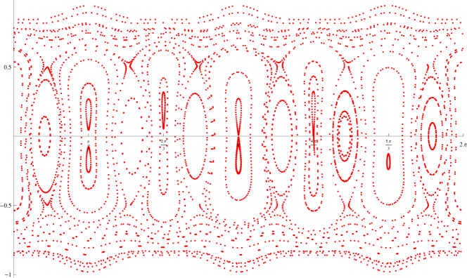
(b)
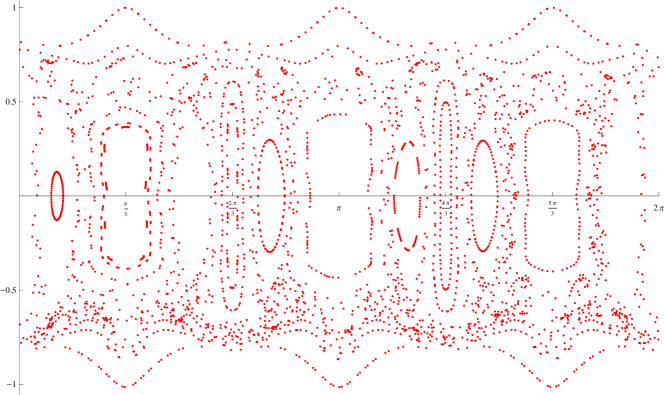
(c)

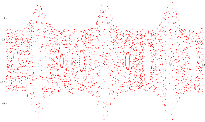
Figure 2: Sample equatorial Poincaré sections for the $n=3$ sectoral harmonic surface, with the following values of $\varepsilon$: (a) $\varepsilon=0.1$; (b) $\varepsilon=0.2$; (c) $\varepsilon=0.3$. The axes are $\phi$ and $\dot{\phi}$. See text for discussion.

The onset of chaotic motion is visible in the Poincaré section of all sectoral harmonic surfaces, with the exception of the $n=1$ surface. On this surface the geodesic flow is perfectly regular for all values of $\varepsilon\in[0,1)$. This is because the $n=1$ sectoral surface is in fact a surface of revolution; it is the surface formed by revolving the limaçon around the $x$-axis, as we may show:

The $n=1$ sectoral surface develops a ‘dimple’ along the $x$-axis. Let us rotate the axes (or alternatively the surface) about the $y$-axis so that the dimple is along the $z$-axis. As this rotation amounts to $(x,y,z)\to(z,y,-x)$ we can define a new set of spherical coordinates $(\overline{\theta},\overline{\phi})$ related to the old spherical coordinates by

$$\sin\theta=\sqrt{1-\sin^{2}\overline{\theta}\cos^{2}\overline{\phi}},\quad\cos\phi=\frac{\cos\overline{\theta}}{\sqrt{1-\sin^{2}\overline{\theta}\cos^{2}\overline{\phi}}}.$$

The $n=1$ sectoral harmonic surface is therefore given by

$$r=1+\varepsilon\sin\theta\cos\phi=1+\varepsilon\cos\overline{\theta},$$ (14)

the parametric form of a limaçon, and clearly $\partial r/\partial\overline{\phi}=0$. This surface will therefore have integrable geodesic flow, a fact that will prove useful in the next section as a check of the procedure carried out.

The Poincaré sections provide strong evidence for the following conclusion: the geodesic equations for the sectoral harmonic surfaces with $n>1$ are not integrable. However, the Poincaré sections cannot be used as proof of this statement, for the following reasons:
1) as the break up of regular motion apparently happens only for larger values of $\varepsilon$, there are possibly small values of $\varepsilon$ for which the equations are integrable, as in the general Henon-Heiles system for example [22];
2) the integrations which generate the plots are run over a finite time; if the integrations were run over a longer time interval perhaps a sequence of points which seems to form a closed curve would begin to wander away. This ‘stickiness’ phenomenon is in fact quite common in chaotic systems (see for example Murray and Dermott [24]), and
3) while great pain may be taken to ensure accuracy in numerical investigations, there is no escaping the fact that these are only approximate solutions to a system of nonlinear ODE’s.

Taking these points on board we seek a rigorous and analytical test of the integrability or otherwise of the geodesic equations. This will be the goal of the next section.

4 The variational equations and non-integrability

While proving a dynamical system is integrable is very challenging, and amounts to essentially finding the first integrals, or showing the Hamiltonian is separable in some sense (see for example Ó Mathúna [21]), there are a number of ways of proving a dynamical system is not integrable. This is because integrable systems are very structured, and must admit a number of properties; showing one of these properties does not hold suffices to prove the system is not integrable. While Poincaré famously showed the non-integrability of the 3-body problem over 100 years ago [26], a particularly fruitful modern approach is that due to Morales and Ramis, as expounded in [23],[28] and [29], and applied to the 3-body problem in [8] and [32] among others.

This method focuses on the variational equations which arise from linearizing around a non-constant solution to the dynamical system. In loose terms (which we will define more precisely below), if a Hamiltonian system is integrable then the variational equations will be solvable, in the sense of differential Galois theory. Consequently, if the variational equations are not solvable then the Hamiltonian system is not integrable. This means we need only focus on the variational equations, which is a great advantage as the variational equations are of course linear and therefore much easier to analyse. We will give a brief summary of the required results first.

4.1 Solvability and the Morales-Ramis theorem

Consider the system of linear ordinary differential equations

$$\xi^{\prime}=A\xi,\quad^{\prime}=d/dz$$ (15)

where the elements of $A$ are in some field $K$ (typically the field of meromorphic functions, $\mathbb{C}(z)$). We may construct the Picard-Vessiot extension to this field $L/K$ by adjoining to $K$ the solutions to (15). Associated with (15) is the differential Galois group $\mathcal{G}$ which is the group of automorphisms of $L/K$ which leave fixed the elements of $K$. The linear system is solvable if we may go from the base field $K$ to the field extension $L/K$ by adjoining to $K$

1. integrals,

2. exponentiation of integrals, and

3. algebraic functions

of the elements of $K$ ([23] gives a complete introduction to this topic). Thus we can ‘build’ the solutions to (15) from the elements of the field that the coefficients of (15) belong to, by performing a finite number of ‘allowed’ operations. Solutions of this type may be referred to as closed form or Louivillian solutions, and the differential equation may be called solvable or Louivillian.

We define the variational equations as follows: for the dynamical system $dx/dt=f(x)$ with non-constant solution $\gamma$, we let $x=\gamma+\xi$ and the first variational equations are given by

$$\frac{d\xi}{dt}=\left(\frac{\partial f}{\partial x}\right)_{\gamma}\xi.$$ (16)

The variational equations can be separated into a tangential and a normal component; as autonomous Hamiltonian systems admit the Hamiltonian itself as a first integral this is ‘inherited’ by the tangential variational equation which is therefore always solvable. And now importantly, the normal variational equation will inherit any other first integrals, if they exist, and will therefore also be solvable. This is the Morales-Ramis theorem, which we will quote from [23]:

Theorem (Morales-Ramis).

For a $2n$ dimensional Hamiltonian system assume there are $n$ first integrals which are meromorphic, in involution and independent in the neighborhood of some non-constant solution. Then the identity component of the differential Galois group of the normal variational equation is an abelian subgroup of the symplectic group.

In other words, the normal variational equation (NVE) is solvable in the sense described above. One advantage of the MR theorem is that it considers the differential Galois group $\mathcal{G}$ associated with the differential equation (15), which is a Lie group, rather than the monodromy group used in Ziglin’s theorem, which is discontinuous.

This theorem suggests a procedure for testing the integrability of a Hamiltonian system: find a non-constant solution; linearize around it and separate out the NVE; test the NVE for solvability. If the NVE is not solvable, then the Hamiltonian system is not integrable. To test the solvability of the NVE, we will use the Kovacic algorithm.

4.2 Kovacic algorithm

The Kovacic algorithm can be used to find the closed form solutions of a second order linear ODE with rational coefficients, and is complete in the sense that if the algorithm does not find such solutions then none exist. The original source for the algorithm is Kovacic [20], but see also [14], [29], [4], [1], to name a few, for presentation, discussion, and application of the algorithm. As we will see, the NVE associated with the system studied in this work will be Fuchsian, which allows for a more concise version of the algorithm. As such, we will follow most closely the presentation of the Kovacic algorithm as given in Churchill and Rod [11], and note that the algorithm is also valid in the non-Fuchsian case.

Consider the linear differential equation

$$\xi^{\prime\prime}=r(z)\xi,\quad r\in\mathbb{C}(z).$$ (17)

If this equation is Fuchsian we can write

$$r(z)=\sum_{j=1}^{k}\frac{\beta_{j}}{(z-a_{j})^{2}}+\sum_{j=1}^{k}\frac{\delta_{j}}{z-a_{j}},$$ (18)

where $k$ is the number of finite regular singular points at locations $z=a_{j}$. When $\sum\delta_{j}=0$ then $z=\infty$ is also a regular singular point, with $\beta_{\infty}=\sum(\beta_{j}+\delta_{j}a_{j})$. The indicial exponents are

$$\tau_{j}^{\pm}=\tfrac{1}{2}\left(1\pm\sqrt{1+4\beta_{j}}\right),\quad\tau_{\infty}^{\pm}=\tfrac{1}{2}\left(1\pm\sqrt{1+4\beta_{\infty}}\right)$$

at $z=a_{j}$ and $z=\infty$ respectively. Kovacic [20] proved the following theorem:

Theorem (Kovacic).

Let $\mathcal{G}$ be the differential Galois group associated with (17), and note $\mathcal{G}\in SL(2,\mathbb{C})$. Then only one of four cases can hold:

1. $\mathcal{G}$ is triangulisable (or reducible), in which case (17) has a solution of the form $\xi=e^{\int\omega}$ with $\omega\in\mathbb{C}(z)$ (we could say $\omega$ is algebraic over $\mathbb{C}(z)$ of degree 1);

2. $\mathcal{G}$ is conjugate to a subgroup of

   $$\left\{\begin{pmatrix}\lambda&0\\ 0&\lambda^{-1}\end{pmatrix},\lambda\in\mathbb{C}/\{0\}\right\}\cup\left\{\begin{pmatrix}0&-\beta^{-1}\\ \beta&0\end{pmatrix},\beta\in\mathbb{C}/\{0\}\right\},$$

   in which case (17) has a solution of the form $\xi=e^{\int\omega}$ where $\omega$ is algebraic over $\mathbb{C}(z)$ of degree 2;

3. $\mathcal{G}$ is finite, in which case (17) has a solution of the form $\xi=e^{\int\omega}$ where $\omega$ is algebraic over $\mathbb{C}(z)$ of degree 4, 6 or 12;

4. $\mathcal{G}=SL(2,\mathbb{C})$, in which case (17) is not solvable.

To show the NVE is not solvable, we must check that each of the cases 1-3 cannot hold. If this is the case, then $\mathcal{G}=SL(2,\mathbb{C})$ whose identity component (also $SL(2,\mathbb{C})$) is not abelian, and therefore the original Hamiltonian system is not meromorphically integrable according to the Morales-Ramis theorem.

Kovacic provides an algorithm whereby each case is checked in two stages: first, we consider certain combinations of the indicial exponents and retain all those leading to a non-negative integer $d$, i.e. $d\in\mathbb{N}_{0}$. Second, for each of these values of $d$ we attempt to construct a monic polynomial of degree $d$, or possibly a set of polynomials, which satisfy certain equations. If successful, the solution to (17) can be found. We will state the details for each case in turn:

Case 1 Define the modified indicial exponents

$$\alpha_{j}^{\pm}=\tau_{j}^{\pm}\ \textrm{if}\ \beta_{j}\neq 0;\quad\alpha_{j}^{\pm}=1\ \textrm{if}\ \beta_{j}=0\ \textrm{and}\ \delta_{j}\neq 0;\quad\alpha_{j}^{\pm}=0\ \textrm{if}\ \beta_{j}=\delta_{j}=0,$$

$$\alpha_{\infty}^{\pm}=\tau_{\infty}^{\pm}\ \textrm{if}\ \beta_{\infty}\neq 0;\quad\alpha_{\infty}^{+}=1,\alpha_{\infty}^{-}=0\ \textrm{if}\ \beta_{\infty}=0.$$

Find all combinations of these modified indicial exponents such that

$$d=\alpha_{\infty}^{\pm}-\sum_{j=1}^{k}\alpha_{j}^{\pm}$$

is a non-negative integer. For each $d$ found, look for a monic degree $d$ polynomial $P(z)$ satisfying

$$P^{\prime\prime}+2\theta P^{\prime}+(\theta^{\prime}+\theta^{2}-r)P=0,\quad\theta=\sum_{j=1}^{k}\frac{\alpha_{j}^{\pm}}{z-a_{j}}.$$

If found, a solution to (17) will be $\xi=e^{\int\omega}$ where $\omega=\theta+P^{\prime}/P$.

Case 2 Define the following sets:

$$E_{j}=\{2+e\sqrt{1+4\beta_{j}},e=0,\pm 2\}\cap\mathbb{Z}\ \textrm{if}\ \beta_{j}\neq 0;$$

$$E_{j}=\{4\}\ \textrm{if}\ \beta_{j}=0,\delta_{j}\neq 0;\quad E_{j}=\{0\}\ \textrm{if}\ \beta_{j}=\delta_{j}=0;$$

$$E_{\infty}=\{2+e\sqrt{1+4\beta_{\infty}},e=0,\pm 2\}\cap\mathbb{Z}\ \textrm{if}\ \beta_{\infty}\neq 0;$$

$$E_{\infty}=\{0,2,4\}\ \textrm{if}\ \beta_{\infty}=0.$$

Find all combinations of $e_{j}\in E_{j}$ and $e_{\infty}\in E_{\infty}$, not all even integers, so that

$$d=\frac{1}{2}\Big{(}e_{\infty}-\sum_{j=1}^{k}e_{j}\Big{)}$$

is a non-negative integer. For each $d$ found, look for a monic degree $d$ polynomial $P(z)$ satisfying

$$P^{\prime\prime\prime}+3\theta P^{\prime\prime}+(3\theta^{2}+3\theta^{\prime}-4r)P^{\prime}+(\theta^{\prime\prime}+3\theta\theta^{\prime}+\theta^{3}-4r\theta-2r^{\prime})P=0,\quad\theta=\frac{1}{2}\sum_{j=1}^{k}\frac{e_{j}}{z-a_{j}}.$$

If found, a solution to (17) will be $\xi=e^{\int\omega}$ where $\omega$ is a root of $\omega^{2}+\phi\omega+(\tfrac{1}{2}\phi^{\prime}+\tfrac{1}{2}\phi^{2}-r)=0$ and $\phi=\theta+P^{\prime}/P$.

Case 3 In this case we must follow the procedure below for each of the subcases $N=4,6,12$. Define the following sets:

$$F_{j}=\{6+\tfrac{12e}{N}\sqrt{1+4\beta_{j}},e=0,\pm 1,\ldots,\pm\tfrac{N}{2}\}\cap\mathbb{Z}\ \textrm{if}\ \beta_{j}\neq 0;$$

$$F_{j}=\{12\}\ \textrm{if}\ \beta_{j}=0,\delta_{j}\neq 0;\quad F_{j}=\{0\}\ \textrm{if}\ \beta_{j}=\delta_{j}=0;$$ (19)

$$F_{\infty}=\{6+\tfrac{12e}{N}\sqrt{1+4\beta_{\infty}},e=0,\pm 1,\ldots,\pm\tfrac{N}{2}\}\cap\mathbb{Z}.$$

Find all combinations of $f_{j}\in F_{j}$ and $f_{\infty}\in F_{\infty}$ so that

$$d=\frac{N}{12}\Big{(}f_{\infty}-\sum_{j=1}^{k}f_{j}\Big{)}$$

is a non-negative integer. Now define

$$\theta=\frac{N}{12}\sum_{j=1}^{k}\frac{f_{j}}{z-a_{j}},\quad S=\prod_{i=1}^{k}(z-a_{j}).$$

Let $P_{N}=-P$ where $P(z)$ is a monic polynomial of degree $d$, and recursively define a set of polynomials $P_{N-1},P_{N-2},\ldots,P_{-1}$ in the following way:

$$P_{i-1}=-SP_{i}^{\prime}+[(N-i)S^{\prime}-S\theta]P_{i}-(N-i)(i+1)P_{i+1},\quad i=N,N-1,\ldots,0.$$

If we find $P_{-1}\equiv 0$, then use the set of polynomials $P_{i}$ as coefficients in the following polynomial and find a solution $\omega$:

$$\sum_{i=0}^{N}\frac{S^{i}P_{i}}{(n-i)!}\omega^{i}=0.$$

A solution to (17) will be $\xi=e^{\int\omega}$.

If these three cases fail to produce a closed form solution, it is because such solutions do not exist. We are now in a position to derive the NVE and apply the Kovacic algorithm to it.

4.3 The normal variational equation

First we must derive a non-constant solution to linearize around (there are no constant solutions to geodesic equations). In general, it is a difficult task to find an exact solution to geodesic equations, even for simple symmetrical manifolds. In the case of the sectoral harmonic surfaces however, we are greatly aided by the existence of certain planes of symmetry, leading to planar geodesics. These planes of symmetry play the same role in this context as invariant planes play in more general contexts. In what follows we will take the equatorial planar geodesic as our nominal solution (see Appendix A for some comments on the use of meridianal planar geodesics).

In the equatorial plane $\theta=\tfrac{\pi}{2},\dot{\theta}=0$, the geodesic equation is (from (6),(7) and noting that $\widetilde{\Gamma}^{\theta}_{\phi\phi}=0$, where we use a tilde to denote the value on $\theta=\tfrac{\pi}{2}$)

$$\ddot{\phi}+\widetilde{\Gamma}^{\phi}_{\phi\phi}\ \dot{\phi}^{2}=0$$ (20)

which admits Hamiltonian

$$2\mathcal{H}=\widetilde{g}_{\phi\phi}\dot{\phi}^{2}=1.$$ (21)

To solve for this equatorial planar geodesic we would need to rewrite (21) as

$$\int ds=\int d\phi\sqrt{\widetilde{g}_{\phi\phi}}=\int d\phi\sqrt{(1+\varepsilon\cos(n\phi))^{2}+\varepsilon^{2}n^{2}\sin^{2}(n\phi)}$$ (22)

and solve to find $s=s(\phi)$, then invert this relationship to find $\phi=\phi(s)$. The integrals in (22) can be written in terms of elliptic integrals of various kinds, at least for some values of $n$, however the analysis would benefit from a unified treatment with $n$ as a parameter. That the integrals in (22) are daunting should come as no surprise: we are essentially trying to find the arc-length parameterization of the curve $r=1+\varepsilon\cos(n\phi)$, which we could describe as a limaçon with $n$ ‘lobes’, and there are few curves for which the arc-length is known exactly.

Fortunately we do not need to solve (22) exactly; for the sake of the NVE we can make a change of independent variable which requires then only (21), as we will show. Let us denote the planar geodesic by

$$(\theta,\phi,\dot{\theta},\dot{\phi})=(\tfrac{\pi}{2},\phi_{0},0,\dot{\phi}_{0}),$$ (23)

and let $\theta=\tfrac{\pi}{2}+\xi,\ \phi=\phi_{0}+\eta$. Linearizing around this solution we find the equation in $\ddot{\xi}$ naturally decouples from that of $\ddot{\eta}$, and since the equatorial/invariant plane is given by $\theta=\tfrac{\pi}{2}$ the variation normal to this plane is given by $\xi$, and thus the NVE is

$$\ddot{\xi}= \left(-\widetilde{\Gamma}^{\theta}_{\phi\phi,\theta}\dot{\phi}^{2}\right)\,\xi+\left(-2\widetilde{\Gamma}^{\theta}_{\theta\phi}\dot{\phi}\right)\,\dot{\xi},$$ (24)

where the coefficients are evaluated along the nominal equatorial geodesic. Now we make the change of independent variable $z=\varepsilon\cos(n\phi(s))$ so that

$$\frac{d}{ds}=-\varepsilon n\sin(n\phi)\frac{d\phi}{ds}\frac{d}{dz}=-\frac{\varepsilon n\sin(n\phi)}{\sqrt{\widetilde{g}_{\phi\phi}}}\frac{d}{dz}$$ (25)

and so on. We may replace instances of $\cos(n\phi)$ with $z/\varepsilon$, to give an NVE with rational polynomial coefficients (this process is sometimes referred to as algebrization, and preserves the identity component of the differential Galois group [30]), which we may write as (letting $\xi^{\prime}=d\xi/dz$ etc.)

$$\xi^{\prime\prime}+p(z)\xi^{\prime}+q(z)\xi=0.$$ (26)

Finally, we transform this equation into the standard form required for the Kovacic algorithm

$$\xi^{\prime\prime}=r(z)\xi$$

where

$$r=-q+\tfrac{1}{4}p^{2}+\tfrac{1}{2}p^{\prime}$$

and we extend $z$ to the complex domain. We are now in a position to state the main result of his paper:

Theorem 1.

The geodesic equations for sectoral harmonic surfaces with $n>1$ are not integrable.

Proof.

When $n>1$, the NVE has 6 regular singular points: five finite regular singular points and one at infinity. The finite regular singular points are

$$\{a_{1},\ldots,a_{5}\}=\{-1,\varepsilon,-\varepsilon,\rho_{+},\rho_{-}\}$$ (27)

with

$$\rho_{+/-}=\frac{1\pm n\sqrt{1+\varepsilon^{2}(n^{2}-1)}}{n^{2}-1}.$$ (28)

The case $n=1$ is special, and shall be dealt with below. When $n>1$ and $0<\varepsilon<1$ all singular points are real and distinct. The coefficients in the partial fraction expansion (18) are

$$\beta_{i}=\left\{0,\frac{-3}{16},\frac{-3}{16},\frac{5}{16},\frac{5}{16}\right\},\quad\beta_{\infty}=\frac{n+1}{n^{2}},$$ (29)

and the $\delta_{i}$’s are given in Appendix B; here we need only mention that $\sum\delta_{i}=0$.

We must now check all three cases of the Kovacic algorithm to see is the NVE solvable. Often in the literature some of the cases can be ruled out straight away, based on the “necessary conditions” given in Section 2.1 of Kovacic [20]. However all of these necessary conditions are satisfied in the present case since the order of each pole of $r(z)$ is 2 and moreover

$$\sqrt{1+4\beta_{i}}=\Big{\{}1,\frac{1}{2},\frac{1}{2},\frac{3}{2},\frac{3}{2}\Big{\}}\in\mathbb{Q},\quad\sqrt{1+4\beta_{\infty}}=\frac{n+2}{n}\in\mathbb{Q};$$ (30)

therefore we must examine each case.

The first stage in each case consists of finding all combinations of the $\beta$ coefficients such that $d$ is a non-negative integer. Unfortunately, there are a lot of such combinations. We show the combinations in Table 1, where $N=1$ and $N=2$ represent cases 1 and 2 respectively, and $N=4,6,12$ represent case 3. The values of $n$, the specific sectoral harmonic under consideration, are shown in the column on the left. Each entry in the table gives the possible values of $d$ in bold, and in brackets the number of combinations of indicial exponents which lead to this value of $d$. As can be seen immediately from the table, when $n=7,8,9,11$ and $n>12$ there are no combinations leading to $d\in\mathbb{N}_{0}$; as such the NVE in these cases is not solvable.

For the other values of $n$ we must try to construct a monic polynomial of degree $d$ which solves the required equations. Clearly there are too many to go through individually; for the sake of demonstration we will describe the most involved case, $n=2,N=12$. The relevant sets defined in (19) are

$$F_{1}=\{12\},\quad F_{2}=F_{3}=\{6,7,5,8,4,9,3\},\quad F_{4}=F_{5}=\{6,9,3,12,0,15,-3\},$$

$$F_{\infty}=\{6,8,4,10,2,12,0,14,-2,16,-4,18,-6\}$$ (31)

It is easy to see how there can be many combinations leading to $d\in\mathbb{N}_{0}$. The largest value comes from the combination

$$d=18-(12+3+3-3-3)=6.$$

In this case, we let $P=z^{6}+p_{5}z^{5}+\ldots+p_{0}$, and define

$$P_{12} =-P,$$

$$P_{11} =-SP_{12}^{\prime}-S\theta P_{12},$$

$$P_{10} =-SP_{11}^{\prime}+[S^{\prime}-S\theta]P_{11}-12S^{2}rP_{12},$$

$$P_{9} =\ldots$$

all the way down to $P_{-1}$. These computations quickly become very large and cumbersome. A useful note is that each $P_{i}$ is simply a polynomial in $z$, albeit one with very complicated coefficients. The order increases in a regular fashion: since $S=O(z^{k})$, $S\theta=O(z^{k-1})$ and $S^{2}r=O(z^{2(k-1)})$ where $k$ is the number of finite regular singular points, we see that $P_{N}=O(z^{d}),P_{N-1}=O(z^{k-1+d})$ and so on until $P_{-1}=O(z^{(N+1)(k-1)+d})$. In the present case this means $P_{-1}=O(z^{58})$, although the leading coefficient always vanishes. Another useful point is that we only need the first few coefficients in $P_{-1}$; setting the first equal to zero gives a value for $p_{5}$, the second gives a value for $p_{4}$ and so on until we reach a term which cannot be set equal to zero. Then we know that $P_{-1}\not\equiv 0$, which means that this combination for $d$ does not produce a solution.

This procedure has been followed for all combinations listed in Table 1 (using Mathematica). For each and every case, it is not possible to construct the required polynomial $P$. As such, the NVE arising from linearising about an equatorial geodesic on the sectoral harmonic surfaces with $n>1$ does not have a differential Galois group belonging to cases 1,2 or 3 in Kovacic’s theorem; instead, $\mathcal{G}=SL(2,\mathbb{C})$ whose identity component is not abelian. Therefore according to the Morales-Ramis theorem the geodesic equations are not integrable. This ends the proof. ∎

$n$	$N=1$	$N=2$	$N=4$	$N=6$	$N=12$
2	0(4)	0(3), 1(1)	0(4), 1(2),	0(21), 1(10),	0(31), 1(20), 2(13),
			2(1)	2(3), 3(1)	3(8), 4(4), 5(2), 6(1)
3	-	-	-	0(9), 1(3), 2(1)	0(9), 1(6), 2(3),
					3(2), 4(1)
4	-	0(2)	0(2), 1(1)	0(7), 1(2)	0(7), 1(3), 2(2),
					3(1)
5	-	-	-	-	0(2), 1(1)
6	-	-	-	0(3), 1(1)	0(3), 1(2), 2(1)
7	-	-	-	-	-
8	-	-	-	-	-
9	-	-	-	-	-
10	-	-	-	-	0(1)
11	-	-	-	-	-
12	-	-	-	0(2)	0(2), 1(1)

Table 1: The possible values of the non-negative integer $d$; see text for an explanation.

We can now deal with the special case $n=1$:

Theorem 2.

The equatorial NVE on the $n=1$ sectoral harmonic surface is solvable.

Proof.

When $n=1$ the equatorial NVE has five regular singular points, four finite at $a_{j}=\{-1,\varepsilon,-\varepsilon,\rho\}$ with $\rho=-\tfrac{1}{2}(1+\varepsilon^{2})$, and one at infinity. We calculate

$$\beta_{j}=\Big{\{}0,\frac{-3}{16},\frac{-3}{16},\frac{5}{16}\Big{\}},\quad\beta_{\infty}=\frac{45}{16}$$ (32)

and hence

$$\alpha_{j}^{\pm}=\Big{\{}(1,1),\big{(}\tfrac{3}{4},\tfrac{1}{4}\big{)},\big{(}\tfrac{3}{4},\tfrac{1}{4}\big{)},\big{(}\tfrac{5}{4},-\tfrac{1}{4}\big{)},\Big{\}},\quad\alpha_{\infty}^{\pm}=\big{(}\tfrac{9}{4},-\tfrac{5}{4}\big{)}.$$ (33)

There is a combination giving

$$d=\frac{9}{4}-\Big{(}1+\frac{3}{4}+\frac{3}{4}-\frac{1}{4}\Big{)}=0$$ (34)

and since $\theta$ thus defined solves the Riccatti equation $\theta^{\prime}+\theta^{2}-r=0$ we have the pair of Louivillian solutions

$$\xi_{1}=C_{1}(z+1)(z^{2}-\varepsilon^{2})^{3/4}(z-\rho)^{-1/4},\quad\xi_{2}=C_{2}\xi_{1}\int\xi_{1}^{-2}dz.$$ (35)

This is of course entirely as expected since the $n=1$ sectoral surface is a surface of revolution and thus has integrable geodesic flow.

∎

5 Conclusions

The application of Morales-Ramis theory and Poincaré sections, two techniques most often seen in the realm of celestial mechanics and mechanical systems, to study the integrability of geodesic flow presents many interesting possibilities. By choosing a specific class of surfaces to analyze we can rigorously prove the non-integrability of the geodesic equations. It would be of interest to extend the results of this work to examine further surfaces; for example the tesseral harmonics mentioned in Section 2 again have (meridianal) planes of symmetry, and the NVE will have coefficients that contain Legendre polynomials, and in general, it would be very informative if we could examine arbitrary surfaces with a plane of symmetry and try and arrive at some obstructions to integrability. We note that the presence of a plane of symmetry makes the decoupling of the NVE straightforward, however Morales Ruiz [23] outlines a procedure in the absence of an invariant plane. The completeness of the spherical harmonics means that surfaces of a very broad class can be decomposed into a set of spherical harmonics, and perhaps by analyzing these individually we can make some conclusions about their sum. Care must be taken however: the triaxial ellipsoid can be decomposed into a set of (infinite) spherical harmonics, each of which would likely have non-integrable geodesic flow, and yet their recombination gives a surface which is integrable. A further issue to consider is how the surface in question is described; the parametric description of the harmonic surfaces led easily to the calculation of the geodesic equations and in particular the separation of the normal variational equation. If the surface were defined in algebraic form, as is more suited to the double torus for example, this separation may be more problematic. Finally, this subject provides an interesting and fruitful combination of techniques from dynamical systems theory, differential geometry and differential Galois theory.

6 Acknowledgements

The author wishes to thank the School of Mathematics, National University of Ireland, Galway, where some of this work was carried out; Dr. Sergi Simon for useful conversations; and finally the referees for their important and constructive comments.

Appendix A Meridianal sections

The analysis above would carry through were we to use one of the meridianal planes instead of the equatorial plane, with two points to note:

1. When drawing the Poincaré sections, the fact that $\phi=$constant is only a half plane complicates matters. Better to rotate the coordinate system (or surface) to make the meridian an equator. For this we need to rotate the surface about the $x$-axis, and for this we define a new set of coordinates $\vartheta,\varphi$ by

   $$\sin\theta=\sqrt{1-\sin^{2}\vartheta\sin^{2}\varphi},\quad\sin\phi=\frac{\cos\vartheta}{\sin\theta},\quad\cos\phi=\frac{\sin\vartheta\cos\varphi}{\sin\theta}.$$

   Now to write the $n$th sectoral harmonic we expand $\cos(n\phi)$ and then make the replacement; for example, the 3rd sectoral harmonic changes as

   $$\sin^{3}\theta\cos(3\phi)=\sin^{3}\theta(\cos^{3}\phi-3\cos\phi\sin^{2}\phi)=\sin^{3}\vartheta\cos^{3}\varphi-3\sin\vartheta\cos\varphi\cos^{2}\vartheta.$$

   An example of a Poincaré section for this rotated surface is shown below; the same families of closed geodesics can be identified.

   

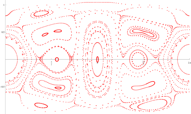
   Figure 3: Sample Poincaré section for the rotated $n=3$ sectoral harmonic surface with $\varepsilon=0.1$. The elliptic nature of the equatorial geodesic (the fixed point at the centre of the plot) can be clearly seen.

2. In deriving the variational equations we may linearize around a meridianal planar geodesic, to derive a normal variational equation of the form given in (26). In the case of an equatorial planar geodesic the denominators of the coefficients are at most quadratic in $z$, however in the case of a meridianal planar geodesic the denominators are polynomials of degree $2n+2$. While the singular points are still regular, the number, location and behaviour of the set of singular points will vary with $n$, complicating matters.

Appendix B Coefficients of equation (18)

$$\delta_{1} =\frac{2}{n(\varepsilon^{2}-1)},$$

$$\delta_{2/3} =\pm\frac{8+n^{2}\pm 2\varepsilon(8+4n+3n^{2})+e^{2}(8+8n+5n^{2}+8n^{3}+4n^{4})}{16\varepsilon(1\pm\varepsilon)^{2}n^{2}},$$

$$\delta_{4/5} =-\frac{1}{2n(1-\varepsilon^{2})^{2}}\left(\varepsilon^{2}(1-2n^{2})-1\pm\big{[}n(1+\varepsilon^{2})\sqrt{1+\varepsilon^{2}(n^{2}-1)}\,\big{]}\right)$$

$$\qquad-\frac{1}{8}\left(\frac{4}{a_{4/5}-a_{1}}+\frac{1}{a_{4/5}-a_{2}}+\frac{1}{a_{4/5}-a_{3}}-\frac{1}{a_{4/5}-a_{5/4}}\right),$$

where the $a_{j}$ are as defined in (27),(28).

Appendix C Bibliography

References

- [1] P. Acosta-Humánez, M. Álvarez Ramírez, and J. Delgado. Non-integrability of some few body problems in two degrees of freedom. Qualitative theory of dynamical systems, 8(2):209–239.
- [2] M. Audin. Hamiltonian aystems and their integrability. American Mathematical Society, 2001.
- [3] V. Bangert. On the existence of closed geodesics on two-spheres. Internat. J. Math., 4(1):1–10, 1993.
- [4] B. Bardin, A. Maciejewski, and M. Przybylska. Integrability of generalized Jacobi problem. Regular and chaotic dynamics, 10(4):437–461, 2005.
- [5] M. V. Berry. Regular and irregular motion. AIP Conference Proceedings, 46:16–120, 1978.
- [6] A. Bolsinov. Integrable geodesic flows on Riemannian manifolds. Journal of Mathematical Sciences, 123(4):4185–4197, 2004.
- [7] A. Bolsinov, V. Kovloz, and A. Fomenko. The maupertius principle and geodesic flows on the sphere arsing from integrable cases of a rigid body. Russian Mathematical Surveys, 50(3):473–501, 1995.
- [8] D. Boucher and J. Weil. Application of the Morales-Ramis theorem to test the non-complete integrability of the planar three-body problem. From combinatorics to dynamical systems, Journées de Calcul Formel, edited by F. Fauvet and C. Mitschi, 2002.
- [9] M. G. Calkin. Lagrangian and Hamiltonian dynamics. World Scientific, 1996.
- [10] M. P. Do Carmo. Differential geometry of curves and surfaces. Prentice-Hall, 1976.
- [11] R. Churchill and D. Rod. On the determination of Ziglin monodromy groups. SIAM J. on Mathematical Analysis, 22(6):1790–1802, 1991.
- [12] C. M. Davison, H. R. Dullin, and A. V. Bolsinov. Geodesics on the ellipsoid and monodromy. Journal of geometry and physics, 57:2437–2454, 2007.
- [13] H. Dullin and V. Matveev. A new integrable system on the sphere. Mathematical research letters, 11:715–722, 2004.
- [14] A. Duval and M. Loday-Richaud. Kovacic’s algorithm and its application to some families of special functions. Applicable algebra in engineering, communication and computation, (3):211–246, 1992.
- [15] J. Franks. Geodesics on and periodic points of annulus homeomorphisms. Invent. Math., 108:403–418, 1992.
- [16] M. Hénon and C. Heiles. The applicability of the third integral of motion: some numerical experiments. The Astronomical Journal, 69(1):73–79, 1964.
- [17] J.V. José and E.J. Saletan. Classical dynamics: a contemporary approach. Cambridge University Press, 1998.
- [18] W. Klingenberg. Riemannian geometry. de Gruyter studies in Mathematics, 1991.
- [19] V. Kolokol’tsov. Geodesic flows on two-dimensional manifolds with an additional first integral that is polynomial in the velocities. Math. USSR Izvestiya, 21(2):291–306, 1983.
- [20] J. Kovacic. An algorithm for solving second order linear homogeneous differential equations. J. symbolic computation, (2):3–43, 1986.
- [21] D. Ó Mathúna. Integrable systems in celestial mechanics. Birkhäuser, 2008.
- [22] J. L. McCauley. Classical mechanics: transformations, flows, integrable and chaotic dynamics. Cambridge University Press, 1997.
- [23] J. J. Morales-Ruiz. Differential Galois theory and non-integrability of Hamiltonian systems. Birkhäuser, 1999.
- [24] C. D. Murray and S. F. Dermott. Solar system dynamics. Cambridge University Press, 2006.
- [25] G. P. Paternain. Geodesic flows. Birkhäuser, 1999.
- [26] H. Poincaré. Les méthodes nouvelles de la mécanique céleste. Gauthier-Villars, 1892, 1893, 1899.
- [27] O. Pujol, J. Pérez, J. Ramis, C. Simó, S. Simon, and J. Weil. Swinging Atwood machine: experimental and numerical results, and a theoretical study. Physica D, 239(12):1067–1081, 2010.
- [28] J. J. Morales Ruiz and Jean Pierre Ramis. Galoisian obstructions to integrability in Hamiltonian systems. Methods of Applications and Analysis, 8(1):33–96, 2001.
- [29] J. J. Morales Ruiz and Jean Pierre Ramis. Galoisian obstructions to integrability in Hamiltonian systems II. Methods of Applications and Analysis, 8(1):97–112, 2001.
- [30] J. Morales Ruiz, C. Simó, and S. Simon. Algebraic proof of the non-integrability of Hill’s problem. Ergodic theory and dynamical systems, 25:1237–1256, 2005.
- [31] A. Thimm. Integrable geodesic flows on homogeneous spaces. Ergodic theory and dynamical systems, 1(4):495–517, 1981.
- [32] A. Tsygvintsev. Non-existence of new meromorphic first integrals in the planar three-body problem. Celestial mechanics and dynamical astronomy, 86(3):237–247, 2003.
- [33] R. M. Wald. General relativity. University of Chicago Press, 1984.
- [34] Z. X. Wang and D. R. Guo. Special functions. World Scientific Publishing, 1989.
- [35] T. Waters. Stability of a 2-dimensional Mathieu-type system with quasiperiodic coefficients. Nonlinear dynamics, 60(3):341–356, 2010.