Jointly Predicting Links and Inferring Attributes using a Social-Attribute Network (SAN)

Abstract

The effects of social influence and homophily suggest that both network structure and node attribute information should inform the tasks of link prediction and node attribute inference. Recently, Yin et al. [28, 29] proposed Social-Attribute Network (SAN), an attribute-augmented social network, to integrate network structure and node attributes to perform both link prediction and attribute inference. They focused on generalizing the random walk with restart algorithm to the SAN framework and showed improved performance. In this paper, we extend the SAN framework with several leading supervised and unsupervised link prediction algorithms and demonstrate performance improvement for each algorithm on both link prediction and attribute inference. Moreover, we make the novel observation that attribute inference can help inform link prediction, i.e., link prediction accuracy is further improved by first inferring missing attributes. We comprehensively evaluate these algorithms and compare them with other existing algorithms using a novel, large-scale Google$+$ dataset, which we make publicly available.

1 Introduction

Online social networks (e.g., Facebook, Google$+$) have become increasingly important resources for interacting with people, processing information and diffusing social influence. Understanding and modeling the mechanisms by which these networks evolve are therefore fundamental issues and active areas of research.

The classical link prediction problem [16] has attracted particular interest. In this setting, we are given a snapshot of a social network at time $t$ and aim to predict links (e.g., friendships) that will emerge in the network between $t$ and a later time $t^{\prime}$. Alternatively, we can imagine the setting in which some links existed at time $t$ but are missing at $t^{\prime}$. In online social networks, a change in privacy settings often leads to missing links, e.g., a user on Google$+$ might decide to hide her family circle between time $t$ and $t^{\prime}$. The missing link problem has important ramifications as missing links can alter estimates of network-level statistics [11], and the ability to infer these missing links raises serious privacy concerns for social networks. Since the same algorithms can be used to predict new links and missing links, we refer to these problems jointly as link prediction.

Another problem of increasing interest revolves around node attributes [31]. Many real-world networks contain rich categorical node attributes, e.g., users in Google$+$ have profiles with attributes including employer, school, occupation and places lived. In the attribute inference problem, we aim to populate attribute information for network nodes with missing or incomplete attribute data. This scenario often arises in practice when users in online social networks set their profiles to be publicly invisible or create an account without providing any attribute information. The growing interest in this problem is highlighted by the privacy implications associated with attribute inference as well as the importance of attribute information for applications including people search and collaborative filtering.

In this work, we simultaneously use network structure and node attribute information to improve performance of both the link prediction and the attribute inference problems, motivated by the observed interaction and homophily between network structure and node attributes. The principle of social influence [7], which states that users who are linked are likely to adopt similar attributes, suggests that network structure should inform attribute inference. Other evidence of interaction [13, 10] shows that users with similar attributes, or in some cases antithetical attributes, are likely to link to one another, motivating the use of attribute information for link prediction. Additionally, previous studies [12, 7] have empirically demonstrated those effects on real-world social networks, providing further support for considering both network structure and node attribute information when predicting links or inferring attributes.

However, the algorithmic question of how to simultaneously incorporate these two sources of information remains largely unanswered. The relational learning [26, 20, 30], matrix factorization and alignment  [19, 24] based approaches have been proposed to leverage attribute information for link prediction, but they suffer from scalability issues. More recently, Backstrom and Leskovec [2] presented a Supervised Random Walk (SRW) algorithm for link prediction that combines network structure and edge attribute information, but this approach does not fully leverage node attribute information as it only incorporates node information for neighboring nodes. For instance, SRW cannot take advantage of the common node attribute San Francisco of $u_{2}$ and $u_{5}$ in Fig. 1 since there is no edge between them.

Yin et al. [29, 28] proposed the use of Social-Attribute Network (SAN) to gracefully integrate network structure and node attributes in a scalable way. They focused on generalizing Random Walk with Restart (RWwR) algorithm to the SAN model to predict links as well as infer node attributes. In this paper, we generalize several leading supervised and unsupervised link prediction algorithms [16, 9] to the SAN model to both predict links and infer missing attributes. We evaluate these algorithms on a novel, large-scale Google$+$ dataset, and demonstrate performance improvement for each of them. Moreover, we make the novel observation that inferring attributes could help predict links, i.e., link prediction accuracy is further improved by first inferring missing node attributes.

2 Problem Definition

In our problem setting, we use an undirected graph $G=(V,E)$ to represent a social network, where edges in $E$ represent interactions between the $N=|V|$ nodes in $V$. In addition to network structure, we have categorical attributes for nodes. For instance, in the Google$+$ social network, nodes are users, edges represent friendship (or some other relationship) between users, and node attributes are derived from user profile information and include fields such as employer, school, and hometown. In this work we restrict our focus to categorical variables, though in principle other types of variables, e.g., live chats, email messages, real-valued variables, etc., could be clustered into categorical variables via vector quantization, or directly discretized to categorical variables.

We use a binary representation for each categorical attribute. For example, various employers (e.g., Google, Intel and Yahoo) and various schools (e.g., Berkeley, Stanford and Yale) are each treated as separate binary attributes. Hence, for a specific social network, the number of distinct attributes $M$ is finite (though $M$ could be large). Attributes of a node $u$ are then represented as a $M$-dimensional trinary column vector $\vec{a}_{u}$ with the $i^{th}$ entry equal to $1$ when $u$ has the $i^{th}$ attribute (positive attribute), $-1$ when $u$ does not have it (negative attribute) and $0$ when it is unknown whether or not $u$ has it (missing attribute). We denote by $A=[\vec{a}_{1}\ \vec{a}_{2}\cdot\cdot\cdot\vec{a}_{N}]$ the attribute matrix for all nodes. Note that certain attributes (e.g. Female and Male, age of 20 and 30) are mutually exclusive. Let $L$ be the set of all pairs of mutually exclusive attributes. This set constrains the attribute matrix $A$ so that no column contains a $1$ for two mutually exclusive attributes.

We define the link prediction problem as follows:

Definition 1 (Link Prediction Problem)

Let $T_{i}=(G_{i},A_{i},L_{i})$ and $T_{j}=(G_{j},A_{j},L_{j})$ be snapshots of a social network at times $i$ and $j$. Then the link prediction problem involves using $T_{i}$ to predict the social network structure $G_{j}$. When $i<j$, new links are predicted. When $i>j$, missing links are predicted.

In this paper, we work with three snapshots of the Google$+$ network crawled at three successive times, denoted $T_{1}=(G_{1},A_{1},L_{1})$, $T_{2}=(G_{2},A_{2},L_{2})$ and $T_{3}=(G_{3},A_{3},L_{3})$. To predict new links, we use various algorithms to solve the link prediction problem with $i=2$ and $j=3$ and first learn any required hyperparameters by performing grid search on the link prediction problem with $i=1$ and $j=2$. Similarly, to predict missing links, we solve the link prediction problem with $i=2$ and $j=1$ and learn hyperparameters via grid search with $i=3$ and $j=2$.

For any given snapshot, several entries of $A$ will be zero, corresponding to missing attributes. The attribute inference problem, which involves only a single snapshot of the network, is defined as follows:

Definition 2 (Attribute Inference Problem)

Let $T=(G,A,L)$ be a snapshot of a social network. Then the attribute inference problem is to infer whether each zero entry of $A$ corresponds to a positive or negative attribute, subject to the constraints listed in $L$.

Our goal is to design scalable algorithms leveraging both network structure and rich node attributes to address these problems for real-world large-scale networks.

3 Model and Algorithms

3.1 Social-Attribute Network Model

Social-Attribute Network was first proposed by Yin et al. [28, 29] to predict links and infer attributes. However, their original model didn’t consider negative and mutually exclusive attributes. In this section, we review this model and extend it to incorporate negative and mutex attributes.

Given a social network $G$ with $M$ distinct categorical attributes, an attribute matrix $A$ and mutex attributes set $L$, we create an augmented network by adding $M$ additional nodes to $G$, with each additional node corresponding to an attribute. For each node $u$ in $G$ with positive or negative attribute $a$, we create an undirected link between $u$ and $a$ in the augmented network. For each mutually exclusive attribute pair $(a,b)$, we create an undirected link between $a$ and $b$. This augmented network is called the Social-Attribute Network (SAN) since it includes the original social network interactions, relations between nodes and their attributes and mutex links between attributes.

Nodes in the SAN model corresponding to nodes in $G$ are called social nodes, and nodes representing attributes are called attribute nodes. Links between social nodes are called social links, and links between social nodes and attribute nodes are called attribute links. Attribute link $(u,a)$ is a positive attribute link if $a$ is a positive attribute of node $u$, and it is a negative attribute link otherwise. Links between mutually exclusive attribute nodes are called mutex links. Intuitively, the SAN model explicitly describes the sharing of attributes across social nodes as well as the mutual exclusion between attributes, as illustrated in the sample SAN model of Fig. 1. Moreover, with the SAN model, the link prediction problem reduces to predicting social links and the attribute inference problem involves predicting attribute links.

We also place weights on the various nodes and edges in the SAN model. These node and edge weights describe the relative importance of individual nodes or relationships across nodes and can also be used in a global fashion to balance the influence of social nodes versus attribute nodes and social links versus attribute links. We use $w(u)$ and $w(u,v)$ to denote the weight of node $u$ and the weight of link $(u,v)$, respectively. Additionally, for a given social or attribute node $u$ in the SAN model, we denote by $\Gamma_{+}(u)$ and $\Gamma_{s+}(u)$ respectively the set of all neighbors and the set of social neighbors connected to $u$ via social links or positive attribute links. We define $\Gamma_{-}(u)$ and $\Gamma_{s-}(u)$ in a similar fashion. This terminology will prove useful when we describe our generalization of leading link prediction algorithms to the SAN model in the next section.

The fact that no social node can be linked to multiple mutex attributes is encoded in the mutex property, i.e., there is no triangle consisting of a mutex link and two positive attribute links in any social-attribute network, which enforces a set of constraints for all attribute inference algorithms.

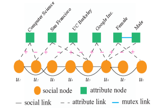
Figure 1: Illustration of a Social-Attribute Network (SAN). The link prediction problem reduces to predicting social links while the attribute inference problem involves predicting attribute links.

In this work, we focus primarily on node attributes. However, we note that the SAN model can be naturally extended to incorporate edge attributes. Indeed, we can use a function (e.g., the logistic function) to map a given set of attributes for each edge (e.g., edge age) into the real-valued edge weights of the SAN model. The attributes-to-weight mapping function can be learned using an approach similar to the one proposed by Backstrom and Leskovec [2].

3.2 Algorithms

Link prediction algorithms typically compute a probabilistic score for each candidate link and subsequently rank these scores and choose the largest ones (up to some threshold) as putative new or missing links. In the following, we extend both unsupervised and supervised algorithms to the SAN model. Furthermore, we note that when predicting attribute links, the SAN model features a post-processing step whereby we change the lowest ranked putative positive links violating the mutex property to negative links.

3.2.1 Unsupervised Link and Attribute Inference

Liben-Nowell and Kleinberg [16] provide a comprehensive survey of unsupervised link prediction algorithms for social networks. These algorithms can be roughly divided into two categories: local-neighborhood-based algorithms and global-structure-based algorithms. In principle, all of the algorithms discussed in [16] can be generalized for the SAN model. In this work we focus on representative algorithms from both categories and we describe below how to generalize them to the SAN model to predict both social links and attribute links. We add the suffix ‘-SAN’ to each algorithm name to indicate its generalization to the SAN model. In our presentation of the unsupervised algorithms, we only consider positive attribute links, though many of these algorithms can be extended to signed networks [25].

Common Neighbor (CN-SAN) is a local algorithm that computes a score for a candidate social or attribute link $(u,v)$ as the sum of weights of $u$ and $v$’s common neighbors, i.e. $score(u,v)=\sum_{t\in\Gamma_{+}(u)\cap\Gamma_{+}(v)}w(t)$. Conventional CN only considers common social neighbors.

Adamic-Adar (AA-SAN) is also a local algorithm. For a candidate social link $(u,v)$ the AA-SAN score is

$$score(u,v)=\sum_{t\in\Gamma_{+}(u)\cap\Gamma_{+}(v)}\frac{w(t)}{\log|\Gamma_{s+}(t)|}\,.$$

Conventional AA, initially proposed in [1] to predict friendships on the web and subsequently adapted by [16] to predict links in social networks, only considers common social neighbors. AA-SAN weights the importance of a common neighbor proportional to the inverse of the log of social degree. Intuitively, we want to downweight the importance of neighbors that are either i) social nodes that are social hubs or ii) attribute nodes corresponding to attributes that are widespread across social nodes. Since in both cases this weight depends on the social degree of a neighbor, the AA-SAN weight is derived based on social degree, rather than total degree.

In contrast, for a candidate attribute link $(u,a)$, the attribute degree of a common neighbor does influence the importance of the neighbor. For instance, consider two social nodes with the same social degree that are both common neighbors of nodes $u$ and $a$. If the first of these social nodes has only two attribute neighbors while the second has $1000$ attribute neighbors, the importance of the former social node should be greater with respect to the candidate attribute link. Thus, AA-SAN computes the score for candidate attribute link $(u,a)$ as

$$score(u,a)=\sum_{t\in\Gamma_{s+}(u)\cap\Gamma_{s+}(a)}\frac{w(t)}{\log|\Gamma_{+}(t)|}\,.$$

Low-rank Approximation (LRA-SAN) takes advantage of global structure, in contrast to CN-SAN and AA-SAN. Denote $X_{S}$ as the $N\times N$ weighted social adjacency matrix where the $(u,v)th$ entry of $X_{S}$ is $w(u,v)$ if $(u,v)$ is a social link and zero otherwise. Similarly, let $X_{A}$ be the $N\times M$ weighted attribute adjacency matrix where the $(u,a)th$ entry of $X_{A}$ is $w(u,a)$ if $(u,a)$ is a positive attribute link and zero otherwise. We then obtain the weighted adjacency matrix $X$ for the SAN model by concatenating $X_{S}$ and $X_{A}$, i.e., $X=[X_{S}\ X_{A}]$. The LRA-SAN method assumes that a small number of latent factors (approximately) describe the social and attribute link strengths within $X$ and attempts to extract these factors via low-rank approximation of $X$, denoted by $\hat{X}$. The LRA-SAN score for a candidate social or attribute link $(u,t)$ is then simply $\hat{X}_{ut}$, or the $(u,t)th$ entry of $\hat{X}$. LRA-SAN can be computed efficiently via truncated Singular Value Decomposition (SVD).

CN + Low-rank Approximation (CN+LRA-SAN) is a mixture of local and global methods, as it first performs CN-SAN using a SAN model and then performs low-rank approximation on the resulting score matrix. After performing CN-SAN, let $S_{S}$ be the resulting $N\times N$ score matrix for all social node pairs and $S_{A}$ be the resulting $N\times M$ score matrix for all social-attribute node pairs. By virtue of the CN-SAN algorithm, note that $S_{S}$ includes attribute information and $S_{A}$ includes social interactions. CN+LRA-SAN then predicts social links by computing a low-rank approximation of $S_{S}$ denoted $\hat{S}_{S}$, and each entry of $\hat{S}_{S}$ is the predicted social link score. Similarly, $\hat{S}_{A}$ is a low-rank approximation of $S_{A}$, and each entry of $\hat{S}_{A}$ is the predicted score for the corresponding attribute link.

AA + low-rank Approximation(AA+LRA-SAN) is identical to CN+LRA-SAN but with the score matrices $S_{S}$ and $S_{A}$ generated via the AA-SAN algorithm.

Random Walk with Restart (RWwR-SAN) [29] is a global algorithm. In the SAN model, a Random Walk with Restart  [4, 21] starting from $u$ recursively walks to one of its neighbors $t$ with probability proportional to the link weight $w(u,t)$ and returns to $u$ with a fixed restart probability $\alpha$. The probability $P_{u,v}$ is the stationary probability of node $v$ in a random walk with restart initiated at $u$. In general, $P_{u,v}\neq P_{v,u}$. For a candidate social link $(u,v)$, we compute $P_{u,v}$ and $P_{v,u}$ and let $score(u,v)=(P_{u,v}+P_{v,u})/2$. Note that RWwR for link prediction in previous work [16] computes these stationary probabilities based only on the social network. For a candidate attribute link $(u,a)$, RWwR-SAN only computes $P_{u,a}$, and $P_{u,a}$ is taken as the score of $(u,a)$.

We finally note that for predicting social links, if we set the weights of all attribute nodes and all attribute links to zero and we set the weights of all social nodes and social links to one, then all the algorithms described above reduce to their standard forms described in [16]. In other words, we recover the link prediction algorithms on pure social networks.

3.2.2 Supervised Link and Attribute Inference

Link prediction can be cast as a binary classification problem, in which we first construct features for links, and then use a classifier such as SVMs or Logistic Regression. In contrast to unsupervised attribute inference, negative attribute links are needed in supervised attribute inference.

Supervised Link Prediction (SLP-SAN) For each link in our training set, we can extract a set of topological features $F$ (e.g. CN, AA, etc.) computed from pure social networks and the similar features $F\_SAN$ computed from the corresponding social-attribute networks. We explored 4 feature combinations: i) SLP-I uses only topological features $F$ computed from social networks; ii) SLP-II uses topological features $F$ as well as an aggregate feature, i.e., the number of common attributes of the two endpoints of a link; iii) SLP-SAN-III uses topological features $F\_SAN$; and iv) SLP-SAN-VI uses topological features $F$ and $F\_SAN$. SLP-SAN-III and SLP-SAN-VI contain the substring ‘SAN’ because they use features extracted from the SAN model. SLP-I and SLP-II are widely used in previous work [9, 17, 2].

Supervised Attribute Inference (SAI-SAN) Recall that attribute inference is transformed to attribute link prediction with the SAN model. We can extract a set of topological features for each positive and negative attribute link. Moreover, the positive attribute links are taken as positive examples while the negative attribute links are taken as negative examples. Hence, we can train a binary classifier for attribute links and then apply it to infer the missing attribute links.

3.2.3 Iterative Link and Attribute Inference

In many real-world networks, most node attributes are missing. Fig. 2 shows the fraction of users as a function of the number of node attributes in Google$+$ social network. From this figure, we see that roughly 70% of users have no observed node attributes. Hence, we will also investigate an iterative variant of the SAN model. We first infer the top attributes for users without any observed attributes. We then update the SAN model to include these predicted attributes and perform link prediction on the updated SAN model. This process can be performed for several iterations.

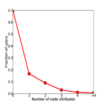
Figure 2: The fraction of users as a function of the number of node attributes in the Google$+$ social network.

4 Google+ Data

Google launched its new social network service named Google$+$ in early July 2011. We crawled three snapshots of the Google$+$ social network and their users’ profiles on July 19, August 6 and September 19 in 2011. They are denoted as JUL, AUG and SEP, respectively. We then pre-processed the data before conducting link prediction and attribute inference experiments.

Preprocessing Social Networks In Google$+$, users divide their social connections into circles, such as a family circle and a friends circle. If user $u$ is in $v$’s circle, then there is a directed edge $(v,u)$ in the graph, and thus the Google$+$ dataset is a directed social graph. We converted this dataset into an undirected graph by only retaining edges $(u,v)$ if both directed edges $(u,v)$ and $(v,u)$ exist in the original graph. We chose to adopt this filtering step for two reasons: (1) Bidirectional edges represent mutual friendships and hence represent a stronger type of relationship that is more likely to be useful when inferring users’ attributes from their friends’ attributes (2) We reduce the influence of spammers who add people into their circles without those people adding them back. Spammers introduce fictitious directional edges into the social graph that adversely influence the performance of link prediction algorithms.

Collecting Attribute Vocabulary Google$+$ profiles include short entries about users such as Occupation, Employment, Education, Places Lived, and Gender, etc. We use Employment and Education to construct a vocabulary of attributes in this paper. We treat each distinct employer or school entity as a distinct attribute. Google$+$ has predefined employer and school entities, although users can still fill in their own defined entities. Due to users’ changing privacy settings, some profiles in JUL are not found in AUG and SEP, so we use JUL to construct our attribute vocabulary. Specifically, from the profiles in JUL, we list all attributes and compute frequency of appearance for each attribute. Our attribute vocabulary is constructed by keeping attributes with frequency of at least 3.

Constructing Social-Attribute Networks In order to demonstrate that the SAN model leverages node attributes well, we derived social-attribute networks in which each node has some positive attributes from the above Google$+$ social networks and attribute vocabulary. Specifically, for an attribute-frequency threshold $k$, we chose the largest connected social network from JUL such that each node has at least $k$ distinct positive attributes. We also found the corresponding social networks consisting of these nodes in snapshots AUG and SEP. Social-attribute networks were then constructed with the chosen social networks and the attributes of the nodes. Specifically, we chose $k=\{2,4\}$ to construct 6 social-attribute networks whose statistics are shown in Table 1. Each social-attribute network is named by concatenating the snapshot name and the attribute-frequency threshold. For example, ‘JUL4’ is the social-attribute network constructed using JUL and $k=4$. These names are indicated in the first column of the table.

In the crawled raw networks, some social links in JUL$i$ are missing in AUG$i$ and SEP$i$, where $i=2,4$. These links are missing due to one of two events occurring between the JUL and AUG or SEP snapshots: 1) users block other users, or 2) users set (part of) their circles to be publicly invisible after which point they cannot be publicly crawled. These missed links provide ground truth labels for our experiments of predicting missing links. However, these missing links can alter estimates of network-level statistics, and can have unexpected influences on link prediction algorithms [11]. Moreover, it is likely in practice that companies like Facebook and Google keep records of these missing links, and so it is reasonable to add these links back to AUG$i$ and SEP$i$ for our link prediction experiments. The third column in Table 1 is the number of all social links after filling the missing links into AUG$i$ and SEP$i$. The second column #soci links is used for experiments of predicting missing links, and column #all soci links is used for the experiments of predicting new links.

From these two columns, the number of new links or missing links can be easily computed. For example, if we use AUG2 as training data and SEP2 as testing data for link prediction, the number of new links is $354572-339059=15513$, which is computed with entries in column #all soci links. If we use AUG2 as training data and JUL2 as testing data in predicting missing links, the number of missing links is $339059-328761=10298$, which is computed with corresponding entries in column #soci links and #all soci links.

Table 1: Statistics of social-attribute networks.

	#soci links	#all soci links	#soci nodes	#pos attri links	#attri nodes
JUL4	7062	7062	5200	24690	9539
AUG4	7430	7813
SEP4	7422	8100
JUL2	287906	287906	170002	442208	47944
AUG2	328761	339059
SEP2	332398	354572

5 Experiments

Table 2: Results for predicting new links. (a)AUC of hop-2 new links on the train-test pair AUG4-SEP4. (b)AUC of hop-2 new links on the train-test pair AUG2-SEP2. (c) (d) AUC of any hop new links on the train-test pair AUG4-SEP4. The numbers in parentheses are standard deviations.

Alg	w/o Attri	With Attri
Random	0.5000	0.5000
CN-SAN	0.6730	0.7315
AA-SAN	0.7109	0.7476
LRA-SAN	0.6003	0.6262
CN+LRA-SAN	0.6969	0.7671
AA+LRA-SAN	0.7118	0.7471
RWwR-SAN	0.6033	0.6143

(a)

Alg	w/o Attri	With Attri
Random	0.5000	0.5000
CN-SAN	0.6936	0.7508
AA-SAN	0.7638	0.7895
LRA-SAN	0.6410	0.6385
CN+LRA-SAN	0.5642	0.6373
AA+LRA-SAN	0.6032	0.6557
RWwR-SAN	0.6788	0.6912

(b)

Alg	w/o Attri	With Attri
Random	0.5000	0.5000
CN-SAN	0.7482	0.8298
AA-SAN	0.7483	0.8324
LRA-SAN	0.8075	0.8237
CN+LRA-SAN	0.7857	0.8651
AA+LRA-SAN	0.8193	0.8552
RWwR-SAN	0.9363	0.9548

(c)

Alg	AUC
SLP-I	0.9128(0.0140)
SLP-II	0.9580(0.0017)
SLP-SAN-III	0.9450(0.0007)
SLP-SAN-VI	0.9706(0.0004)
SRW	0.9383

(d)

5.1 Experimental Setup

In our experiments, the main metric used is AUC, Area Under the Receiver Operating Characteristic (ROC) Curve, which is widely used in the machine learning and social network communities [5, 2]. AUC is computed in the manner described in [8], in which both positive and negative examples are required. In principle, we could use new links or missing links as positive examples and all non-existing links as negative examples. However, large-scale social networks tend to be very sparse, e.g., the average degree is $4.17$ in SEP2, and, as a result, the number of non-existing links can be enormous, e.g., SEP2 has around $2.9\times 10^{10}$ non-existing links. Hence, computing AUC using all non-existing links in large-scale networks is typically computationally infeasible. Moreover, the majority of new links in typical online social networks close triangles [14, 2], i.e., are hop-2 links. For instance, we find that $58\%$ of the newly added links in Google+ are hop-2 links. We thus evaluate our large network experiments using hop-2 link data as in [2], i.e., new or missing hop-2 links are treated as positive examples and non-existing hop-2 links are treated as negative examples.

In a social-attribute network, there are two categories of hop-2 links: 1) those with two endpoints sharing at least one common social node, and 2) those with two endpoints sharing only common attribute nodes. Local algorithms applied to the original social network are unable to predict hop-2 links in the second category. Thus, we evaluate only with respect to hop-2 links in the first category, so as not to give unfair advantage to algorithms running on the social-attribute network. To better understand whether the AUC performance computed on hop-2 links can be generalized to performance on any-hop links, we additionally compute AUC using any-hop links on the smaller Google$+$ networks.

In general, different nodes and links can have different weights in social-attribute networks, representing their relative importance in the network. In all of our experiments in this paper, we set all weights to be one and leave it for future work to learn weights.

We compare our link prediction algorithms with Supervised Random Walk (SRW) [2], which leverages edge attributes, by transforming node attributes to edge attributes. Specifically, we compute the number of common attributes of the two endpoints of each existing link. As in [2], we also use the number of common neighbors as an edge attribute. We adopt the Wilcoxon-Mann-Whitney (WMW) loss function and logistic edge strength function in our implementations as recommended in [2].

We compare our attribute inference algorithms with two algorithms, BASELINE and LINK, introduced by Zheleva and Getoor [31]. Using only node attributes, BASELINE first computes a marginal attribute distribution and then uses an attribute’s probability as its score. LINK trains a classifier for each attribute by flattening nodes as the rows of the adjacency matrix of the social networks. Zheleva and Getoor [31] found that LINK is the best algorithm when group memberships are not available.

We use SVM as our classifier in all supervised algorithms. For link prediction, we extract six topological features (CN-SAN, AA-SAN, LRA-SAN, CN+LRA-SAN, AA+LRA-SAN and RWwR-SAN) from both pure social networks and social-attribute networks. Hence, SLP-I, SLP-II, SLP-SAN-III and SLP-SAN-VI use 6, 7, 6 and 12 features, respectively. For attribute inference, we extract 9 topological features for each attribute link. We adopt two ranks (detailed in 5.2.2) for each low-rank approximation based algorithms, thus obtaining 6 features. The other three features are CN-SAN, AA-SAN and RWwR-SAN. To account for the highly imbalanced class distribution of examples for supervised link prediction and attribute inference we downsample negative examples so that we have equal number of positive and negative examples (techniques proposed in  [17, 6] could be used to further improve the performance).

We use the pattern dataset1-dataset2 to denote a train-test or train-validation pair, with dataset1 a training dataset and dataset2 a testing or validation dataset. When conducting experiments to predict new links on the AUG$i$-SEP$i$ train-test pair, SRW, classifiers and hyperparameters of global algorithms, i.e., ranks in LRA-SAN, CN+LRA-SAN, and AA+LRA-SAN and the restart probability $\alpha$ in RWwR-SAN, are learned on the JUL$i$-AUG$i$ train-validation pair. Similarly, when predicting missing links on train-test pair AUG$i$-JUL$i$, they are learned on train-validation pair SEP$i$-AUG$i$, where $i=2,4$.

The CN-SAN and AA-SAN algorithms are implemented in Python 2.7 while the RWwR-SAN algorithm and Supervised Random Walk (SRW) are implemented in Matlab, and all of them are run on a desktop with a 3.06 GHz Intel Core i3 and 4GB of main memory. LRA-SAN, CN+LRA-SAN and AA+LRA-SAN algorithms are implemented in Matlab and run on an x86-64 architecture using a single 2.60 Ghz core and 30GB of main memory.

5.2 Experimental Results

In this section we present evaluations of the algorithms on the Google+ dataset. We first show that incorporating attributes via the SAN model improves the performance of both unsupervised and supervised link prediction algorithms. Then we demonstrate that inferring attributes via link prediction algorithms within the SAN model achieves state-of-the-art performance. Finally, we show that by combining attribute inference and link prediction in an iterative fashion, we achieve even greater accuracy on the link prediction task.

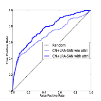
Figure 3: ROC curves of the CN+LRA-SAN algorithm for predicting new links. AUG4-SEP4 is the train-test pair. JUL4-AUG4 is the train-validation pair.

5.2.1 Link Prediction

To demonstrate the benefits of combining node attributes and network structure, we run the SAN-based link prediction algorithms described in Section 3.2 both on the original social networks and on the corresponding social-attribute networks (recall that the SAN-based unsupervised algorithms reduce to standard unsupervised link prediction algorithms when working solely with the original social networks).

Predicting New Links Table 2d shows the AUC results of predicting new links for each of our datasets. We are able to draw a number of conclusions from these results. First, the SAN model improves every unsupervised learning algorithm on every dataset, save for LRA-SAN on AUG2-SEP2. Second, Table 2d shows that attributes also improve supervised link prediction performance since SLP-SAN-VI, SLP-SAN-III and SLP-II outperform SLP-I. Moreover, SLP-SAN-VI, which adopts features extracted from both social networks and social-attribute networks, achieves the best performance, thus demonstrating the power of the SAN model. Third, comparing RWwR-SAN in Table 2c and SRW in Table 2d, we observe that the SAN model is better than SRW at leveraging node attributes since RWwR-SAN with attributes outperforms SRW. This result is not surprising given that SRW is designed for edge attributes and when transforming node attributes to edge attributes, we lose some information. For instance, as illustrated in Fig. 1, nodes $u_{2}$ and $u_{5}$ share the attribute San Francisco. When transforming node attributes to edge attributes, this common attribute information is lost since $u_{2}$ and $u_{5}$ are not linked.

Fig. 3 shows the ROC curves of the CN+LRA-SAN algorithm. We see that curve of CN+LRA-SAN with attributes dominates that of CN+LRA-SAN without attributes, demonstrating the power of the SAN model to effectively incorporate the additional predictive information of attributes.

Table 3: Results for predicting missing links. (a) AUC of hop-2 missing links on the train-test pair AUG4-JUL4. (b) AUC of hop-2 missing links on the train-test pair AUG2-JUL2. (c)-(f) AUC of any-hop missing links on the train-test pair AUG4-JUL4. Missing links in both categories 1 and 2 are used in (c) and (d). Missing links in Category 1 are used in (e) and (f). The numbers in parentheses are standard deviations.

Alg	w/o Attri	With Attri
Random	0.5000	0.5000
CN-SAN	0.7180	0.7925
AA-SAN	0.7437	0.7697
LRA-SAN	0.6569	0.6237
CN+LRA-SAN	0.7147	0.7986
AA+LRA-SAN	0.7410	0.7668
RWwR-SAN	0.5731	0.5676

(a)

Alg	w/o Attri	With Attri
Random	0.5000	0.5000
CN-SAN	0.6938	0.7309
AA-SAN	0.7633	0.7796
LRA-SAN	0.6044	0.6059
CN+LRA-SAN	0.5816	0.6266
AA+LRA-SAN	0.6212	0.6569
RWwR-SAN	0.6595	0.6706

(b)

Alg	AUC
SLP-I	0.5453(0.0120)
SLP-II	0.6991(0.0065)
SLP-SAN-III	0.7161(0.0030)
SLP-SAN-VI	0.8481(0.0022)

(c)

Alg	w/o Attri	With Attri
Random	0.5000	0.5000
CN-SAN	0.5460	0.7012
AA-SAN	0.5460	0.7033
LRA-SAN	0.5495	0.6177
CN+LRA-SAN	0.5547	0.7048
AA+LRA-SAN	0.5640	0.7325
RWwR-SAN	0.2000	0.7619

(d)

Alg	w/o Attri	With Attri
Random	0.5000	0.5000
CN-SAN	0.7329	0.7765
AA-SAN	0.7330	0.7784
LRA-SAN	0.7316	0.7401
CN+LRA-SAN	0.7515	0.7510
AA+LRA-SAN	0.8104	0.8116
RWwR-SAN	0.7797	0.8838

(e)

Alg	AUC
SLP-I	0.8023(0.0088)
SLP-II	0.8403(0.0033)
SLP-SAN-III	0.8620(0.0080)
SLP-SAN-VI	0.8854(0.0324)

(f)

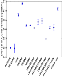
(a)

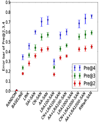
(b)

Figure 4: Performance of various algorithms on attribute inference on SEP4. (a) AUC under ROC curves. (b) Pre@2,3,4.

Predicting Missing Links Missing links can be divided into two categories: 1) links whose two endpoints have some social links in the training dataset. 2) links with at least one endpoint that has no social links in the training dataset. Category 1 corresponds to the scenarios where users block users or users set a part of their friend lists (e.g. family circles) to be private. Category 2 corresponds to the scenario in which users hide their entire friend lists. Note that all hop-2 missing links belong to Category 1. In addition to performing experiments to show that the SAN model improves missing link prediction, we also perform experiments to explore which category of missing links is easier to predict. Table 3f shows the results of predicting missing links on various datasets. As in the new-link prediction setting, the performance of every algorithm is improved by the SAN model, except for LRA-SAN on AUG4-JUL4 and RWwR-SAN on AUG4-JUL4 for hop-2 missing links.

When comparing Tables 3d and 3e or Tables 3c and 3f, we conclude that the missing links in Category 2 are harder to predict than those in Category 1. RWwR-SAN without attributes performs poorly when predicting any-hop missing links in both categories (as indicated by the entry with $0.2000$ in Table 3d). This poor performance is due to the fact that RWwR-SAN without attributes assigns zero scores for all the missing links in Category 2 (positive examples) and positive scores for most non-existing links (negative examples), making many negative examples rank higher than positive examples and resulting in a very low AUC.

5.2.2 Attribute Inference

In this section, we focus on inferring attributes using the SAN model. In our next set of experiments in Section 5.2.3, we use the results of these attribute inference algorithms to further improve link prediction, and the results of this iterative approach further validate the performance of the SAN model for attribute inference. Since the first step of iterative approach of Section 5.2.3 involves inferring the top attributes for each node, we employ an additional performance metric called Pre@$K$ in our attribute inference experiments. Compared to AUC, Pre@$K$ better captures the quality of the top attribute predictions for each user. Specifically, for each sampled user, the top-$K$ predicted attributes are selected, and (unnormalized) Pre@$K$ is then defined as the number of positive attributes selected divided by the number of sampled users. We address score ties in the manner described in [18]. Since most Google$+$ users have a small number of attributes, we set $K=2,3,4$ in our experiments.

When evaluating algorithms for the inference of missing attributes, we require ground truth data. In general, ground truth for node attributes is difficult to obtain since it is often not possible to distinguish between negative and missing attributes. However, for most users the number of attributes is quite small, and so we assume that users with many positive attributes have no missing attributes. Hence, we evaluate attribute inference on users that have at least 4 specified attributes, i.e., we work with users in SEP4 and assume that each attribute link in SEP4 is either positive or negative.

In our experiment, we sample 10% of the users in SEP4 uniformly at random, remove their attribute links from SEP4, and evaluate the accuracy with which we can infer these users’ attributes. All removed positive attribute links are viewed as positive examples, while all the negative attribute links of the sampled users are treated as negative examples. We run a variety of algorithms for attribute inference, and for each algorithm we average the results over 10 random trials. As noted above, we evaluate the performance of attribute inference using both AUC and Pre@$K$.

For the low-rank approximation based algorithms, i.e., LRA-SAN, CN+LRA-SAN and AA+LRA-SAN, we report results using two different ranks, 100 and 1000, and indicate which was used by the number following the algorithm name in Fig. 4. We choose these two small ranks for computational reasons and also based on the fact that low-rank approximation methods assume that a small number of latent factors (approximately) describe the social-attribute networks. For RWwR-SAN, we set the restart probability $\alpha$ to be 0.7.

Fig. 4 shows the attribute inference results for various algorithms. Several interesting observations can be made from this figure. First, under both metrics, all SAN-based algorithms perform better than BASELINE, save LRA100-SAN and LRA1000-SAN under Pre@2,3,4 metric, which indicates that the SAN model is good at leveraging network structure to infer missing attributes. Second, we find that AUC and Pre@$K$ provide inconsistent conclusions about relative algorithm performance. For instance, the mean AUC values suggest that SAI-SAN beats all other algorithms. However, several unsupervised algorithms outperform SAI-SAN with respect to Pre@2,3,4. The inconsistencies between the two metrics are expected since AUC is a global measurement while Pre@$K$ is a local one. Our SAI-SAN algorithm dominates LINK under both AUC and Pre@2,3,4 metrics, thus demonstrating the power of mapping attribute inference to link prediction with the SAN model.

Table 4: Results for iteratively inferring attributes and predicting links. (a) on the AUG4-SEP4 train-test pair. (b) on the AUG4-JUL4 train-test pair. Results are averaged over 10 trials. The numbers in parentheses are standard deviations.

Alg	w/o Attri	With Attri	With Inferred Attri
Random	0.5000(0)	0.5000(0)	0.5000(0)
CN-SAN	0.6730(0)	0.7174(0.0077)	0.7291(0.0063)
AA-SAN	0.7109(0)	0.7408(0.0063)	0.7440(0.0026)
LRA-SAN	0.6003(0)	0.6274(0.0052)	0.6320(0.0055)
CN+LRA-SAN	0.6969(0)	0.7497(0.0134)	0.7534(0.0084)
AA+LRA-SAN	0.7111(0)	0.7373(0.0050)	0.7442(0.0032)

(a)

Alg	w/o Attri	With Attri	With Inferred Attri
Random	0.5000(0)	0.5000(0)	0.5000(0)
CN-SAN	0.7180(0)	0.7780(0.0173)	0.7856(0.0100)
AA-SAN	0.7437(0)	0.7626(0.0100)	0.7661(0.0045)
LRA-SAN	0.6569(0)	0.6189(0.0105)	0.6134(0.0157)
CN+LRA-SAN	0.7147(0)	0.7838(0.0256)	0.7969(0.0059)
AA+LRA-SAN	0.7410(0)	0.7591(0.0118)	0.7673(0.0051)

(b)

5.2.3 Iterative Attribute and Link Inference

Section 5.2.1 demonstrated that knowledge of a user’s attributes can lead to significant improvements in link prediction. However, in real-world social networks like Google+, the vast majority of user attributes are missing (see Fig. 2). To increase the realized benefits of social-attribute networks with few attributes, we propose first inferring missing attributes for each user whose attributes are missing and then performing link prediction on the inferred social-attribute networks. Recall that SAI-SAN achieves the best AUC, RWwR-SAN achieves the best Pre@$K$ in inferring attributes (see Fig. 4) and AA-SAN achieves comparable Pre@$K$ results while being more scalable. Thus, in the following experiments, we use AA-SAN to first infer the top-$K$ missing attributes for users, and subsequently perform link prediction using various methods.

In our experiments, when we are working on the pair train-test, we sample 10% of the users of train uniformly at random and remove their attributes. We then run three variants of link prediction algorithms: i) without attributes, ii) with only the remaining attributes, and iii) with the remaining attributes along with the inferred attributes. The top-4 attributes are inferred for each sampled user by AA-SAN. We report the results averaged over 10 trials. The hyperparameters of the global algorithms are the same as those in (Section 5.2.1), which are learned from the corresponding train-validation pair.

Table 4a shows the results of first inferring attributes and then predicting new links on the AUG4-SEP4 train-test pair. Table 4b shows the results of first inferring attributes and then predicting missing links on the AUG4-JUL4 train-test pair. We see that the inferred attributes improve the performance of all algorithms except LRA-SAN on predicting missing links, which is unable to make use of attributes as demonstrated earlier in Table 3a. The AUCs obtained with inferred attributes for all other algorithms are very close to those obtained with all positive attributes as shown in Table 2a. This further demonstrates that AA-SAN is an effective algorithm for attribute inference.

6 Related Work

A wide range of link prediction methods have been developed. Liben-Nowell and Kleinberg [16] surveyed a set of unsupervised link prediction algorithms. Li [15] proposed Maximal Entropy Random Walk (MERW). Lichtenwalter et al. [17] proposed the PropFlow algorithm which is similar to RWwR but more localized. However, none of these approaches leverage node attribute information.

Link prediction methods leveraging attribute information first appear in the relational learning community [26, 20, 3, 30]. However, these approaches suffer from scalability issues. For instance, the largest network tested in [26] has about $3K$ nodes. Recently, Backstrom and Leskovec [2] proposed the Supervised Random Walk (SRW) algorithm to leverage edge attributes. However, SRW does not handle the scenario in which two nodes share common attributes (e.g. nodes $u_{2}$ and $u_{5}$ in Fig. 1), but no edge already exists between them. Mapping link prediction to a classification problem [9, 17, 6] is another way to incorporate attributes. We have shown that classifiers using features extracted from the SAN model perform very well. Yang et al. [27] proposed to jointly predict links and propagate node interests (e.g., music interest). Their algorithm relies on the assumption that each node interest has a set of explicit attributes. As a result, their algorithm cannot be applied to our scenario in which it’s hard (if possible) to extract explicit attributes for our node attributes.

Previous works in [22, 23] aim at inferring node attributes (e.g., ethnicity and political orientation) using supervised learning methods with features extracted from user names and user-generated texts. Zheleva and Getoor [31] map attribute inference to a relational classification problem. They find that methods using group information achieve good results. These approaches are complementary to ours since they use additional information apart from network structure and node attributes. In this paper, we transform the attribute inference problem into a link prediction problem with the SAN model. Therefore, any link prediction algorithm can be used to infer missing attributes. More importantly, we demonstrate that attribute inference can in turn help link prediction with the SAN model.

7 Conclusion and Future Work

We comprehensively evaluate the Social-Attribute Network (SAN) model proposed in [28, 29] in terms of link prediction and attribute inference. More specifically, we adapt several representative unsupervised and supervised link prediction algorithms to the SAN model to both predict links and infer attributes. Our evaluation with a large-scale novel Google$+$ network dataset demonstrates performance improvement for each of these generalized algorithm on both link prediction and attribute inference. Moreover, we demonstrate a further improvement of link prediction accuracy by using the SAN model in an iterative fashion, first to infer missing attributes and subsequently to predict links. Interesting avenues for future research include devising an iterative algorithm that alternates between attribute and link prediction, learning node and edge weights in the SAN model, and incorporating edge attributes, negative node attributes and mutex edges into large-scale experiments.

8 Acknowledgments

We would like to thank Di Wang, Satish Rao, Mario Frank, Kurt Thomas, and Shobha Venkataraman for insightful feedback. This work is supported by the NSF under Grants No. CCF-0424422, 0311808, 0832943, 0448452, 0842694, 0627511, 0842695, 0808617, 1122732, 0831501 CT-L, by the AFOSR under MURI Award No. FA9550-09-1-0539, by the AFRL under grant No. P010071555, by the Office of Naval Research under MURI Grant No. N000140911081, by the MURI program under AFOSR Grant No. FA9550-08-1-0352, the NSF Graduate Research Fellowship under Grant No. DGE-0946797, the DoD through the NDSEG Program, by Intel through the ISTC for Secure Computing, and by a grant from the Amazon Web Services in Education program. Any opinions, findings, and conclusions or recommendations expressed in this material are those of the author(s) and do not necessarily reflect the views of the funding agencies.

References

- [1] L. A. Adamic and E. Adar. Friends and neighbors on the web. Social Network, 25(3):211–230, 2003.
- [2] L. Backstrom and J. Leskovec. Supervised random walks:predicting and recommending links in social networks. In WSDM, 2011.
- [3] M. Bilgic, G. Namata, and Getoor. Combining collective classification and link prediction. In ICDM Workshops, 2007.
- [4] S. Brin and L. Page. The anatomy of a large-scale hypertextual web search engine. Computer Networks and ISDN Systems, 30(1-7):107–117, 1998.
- [5] A. Clauset, C. Moore, and M. E. J. Newman. Hierarchical structure and the prediction of missing links in networks. Nature, 453(7191):98–101, May 2008.
- [6] J. R. Doppa, J. Yu, P. Tadepalli, and L. Getoor. Learning algorithms for link prediction based on chance constraints. In ECML/PKDD, 2010.
- [7] T. L. Fond and J. Neville. Randomization tests for distinguishing social influence and homophily effects. In WWW, 2011.
- [8] D. J. Hand and R. J. Till. A simple generalisation of the area under the roc curve for multiple class classification problems. Machine Learning, 45:171–186, 2001.
- [9] M. A. Hasan, V. Chaoji, S. Salem, and M. Zaki. Link prediction using supervised learning. In SIAM Workshop on Link Analysis, Counterterrorism and Security, 2006.
- [10] M. Kim and J. Leskovec. Modeling social networks with node attributes using the multiplicative attribute graph model. In UAI, 2011.
- [11] G. Kossinets. Effects of missing data in social networks. Social Networks, 28:247–268, 2006.
- [12] G. Kossinets and D. Watts. Empirical analysis of an evolving social network. Science, 2006.
- [13] R. Kumar, J. Novak, P. Raghavan, and A. Tomkins. Structure and evolution of blogspace. Communications of the ACM, 47(12):35–39, 2004.
- [14] J. Leskovec, L. Backstrom, R. Kumar, , and A. Tomkins. Microscopic evolution of social networks. In KDD, 2008.
- [15] R.-H. Li, J. X. Yu, and J. Liu. Link prediction: the power of maximal entropy random walk. In CIKM, 2011.
- [16] D. Liben-Nowell and J. Kleinberg. The link prediction problem for social networks. In CIKM, pages 556–559, 2003.
- [17] R. N. Lichtenwalter, J. T. Lussier, and N. V. Chawla. New perspectives and methods in link prediction. In KDD, 2010.
- [18] F. McSherry and M. Najork. Computing information retrieval performance measures efficiently in the presence of tied scores. In ECIR, 2008.
- [19] A. K. Menon and C. Elkan. Link prediction via matrix factorization. In ECML/PKDD, 2011.
- [20] K. T. Miller, T. L. Griffiths, and M. I. Jordan. Nonparametric latent feature models for link prediction. In NIPS, 2009.
- [21] J.-Y. Pan, H.-J. Yang, C. Faloutsos, and P. Duygulu. Automatic multimedia cross-modal correlation discovery. In KDD, 2003.
- [22] D. Rao, M. Paul, C. Fink, D. Yarowsky, T. Oates, and G. Coppersmith. Hierarchical bayesian models for latent attribute detection in social networks. In ICWSM, 2011.
- [23] D. Rao, D. Yarowsky, A. Shreevats, and M. Gupta. Classifying latent user attributes in twitter. In SMUC, 2010.
- [24] J. Scripps, P.-N. Tan, F. Chen, and A.-H. Esfahanian. A matrix alignment approach for collective classification. In ASONAM, Athens, Greece, 2009.
- [25] P. Symeonidis, E. Tiakas, and Y. Manolopoulos. Transitive node similarity for link prediction in social networks with positive and negative links. In RecSys, 2010.
- [26] B. Taskar, M.-F. Wong, P. Abbeel, and D. Koller. Link prediction in relational data. In NIPS, 2003.
- [27] S. H. Yang, B. Long, A. Smola, N. Sadagopan, Z. Zheng, and H. Zha. Like like alike — joint friendship and interest propagation in social networks. In WWW, 2011.
- [28] Z. Yin, M. Gupta, T. Weninger, and J. Han. Linkrec: a unified framework for link recommendation with user attributes and graph structure. In WWW, 2010.
- [29] Z. Yin, M. Gupta, T. Weninger, and J. Han. A unified framework for link recommendation using random walks. In ASONAM, 2010.
- [30] K. Yu, W. Chu, S. Yu, V. Tresp, and Z. Xu. Stochastic relational models for discriminative link prediction. In NIPS, 2006.
- [31] E. Zheleva and L. Getoor. To join or not to join: The illusion of privacy in social networks with mixed public and private user profiles. In WWW, 2009.