Free Energy Landscape of a Protein-Like Chain in a Fluid with Discontinuous Potentials

Abstract

The free energy landscape of a protein-like chain in a fluid was studied by combining discontinuous molecular dynamics and parallel tempering. The model protein is a repeating sequence of four different beads, with interactions mimicking those in real proteins. Neighbor distances and angles are restricted to physical ranges and one out of the four kinds of beads can form hydrogen bonds with each other, except if they are too close in the chain. In contrast to earlier studies of this model, an explicit square-well solvent is included. Beads that can form intra-chain hydrogen bonds, can also form (weaker) hydrogen bonds with solvent molecules, while other beads are insoluble. By categorizing the protein configurations according to their intra-chain bonds, one can distinguish unfolded, helical, and collapsed helical structures. Simulations for chains of 15, 20 and 25 beads show that at low temperatures, the most likely structures are helical or collapsed helical, despite the low entropy of these structures. The temperature at which helical structures become dominant is higher than in the absence of a solvent. The cooperative effect of the solvent is attributed to the presence of hydrophobic beads. A phase transition of the solvent prevented the simulations of the 20-bead and 25-bead chains of reaching low enough temperatures to confirm whether the free energy landscape is funnel-shaped, although the results do not contradict that possibility.

I Introduction

Proteins have a natural tendency to find a unique folded structure. Understanding how proteins fold, has been a very challenging question in physics, chemistry and biologyshakh:2 ; Science:63 , which remains largely an open problem.

One of the contentious issues is why folding occurs so fast. According to Levinthal, the time required to explore all conformations of an average protein is too long to find the global free energy minimum on realistic time scales.Levinthal:53 ; Wolynes:45 ; Goldstein:55 This seems to clash with the idea that the native configuration of a protein is associated with the global minimum its Gibbs free energy.Wenzel:10 ; Anfinsen:12 To resolve these two apparently conflicting views, it is useful to think of folding as occurring on a free energy landscape. The free energy landscape is the form of the free energy as a function of protein conformation.Wolynes:45 The paradox would be resolved if the landscape has a funnel shape. The system could then slide down the funnel towards the native state through configurations of increasingly lower free energy — much faster than finding the native state through a random walk — but without needing a single, specific kinetic pathway.

There is, furthermore, no consensus as how significant the role of the solvent is for protein folding, or what interaction or set of interactions play the main role.Woolfson:32 Some researchers proposed that folding is a balance between entropy versus enthalpy-dominated hydration.Athawale:13 ; Garde:14 On the other hand, there have been experiments that have shown that a protein can fold into its native configuration with apparently negligible solvent ordering effects.Woolfson:32 ; Soundararajan:73 In many of the theoretical and experimental studies of protein folding, the proteins have been in the absence of a fluid.Rhee:33 However in nature, and therefore in many experimental studies, folding happens in the presence of a fluid environment.

A simple model of a protein without a solvent was studied in Ref. hanif:34, ; we will refer to this work as I below. The simple models in I were used to capture the basic behavior of proteins in a reasonable computational time. This was accomplished by using discontinuous potentials for the attractive and repulsive interaction, as step and shoulder potentials respectively. In addition, here, the protein-like chain is surrounded by an explicit solvent environment. As in I, the investigation of the free energy landscape was done using a Hybrid Monte Carlo (HMC) method, where HMC is implemented as a combination of the Monte Carlo and the Discontinuous Molecular Dynamics (DMD) method. The Parallel Tempering (PT) method Swendsen:6 ; Greyer:7 ; whittington:18 is used for the Monte Carlo part to avoid getting trapped in local free energy minima and to increase the speed of phase space exploration.Earl:8 The PT method allows to generate configurations according to the canonical ensemble.

Our earlier study resulted in a free energy landscape for the protein-like chain in the absence of any fluid. Using a family of simple protein models consisting of a periodic sequence of four different kinds of bead, these protein-like chains exhibited a secondary alpha helix structure in their folded states, and allowed a natural definition of a configuration by considering which beads are bonded. Relative configurational free energies at different temperatures were determined from relative populations at those temperatures.

In the absence of any fluid it could be demonstrated that the energy landscape is rugged at different temperatures and at low enough temperature has a very deep funnel shaped valley especially for the smaller chains. In other words, one structure has a much lower free energy than other structures, so that its probability becomes very high. At the same time, neighboring structures should still have a low free energy, so that folding could be driven through configurations of progressively lower free energy. The much lower free energy of the global minimum was confirmed by the fact that, for chains smaller than 30 beads, the probability of observing the most common configuration was almost one at low enough temperatures.

In this paper we investigate the energy landscape of the protein-like chain in the presence of a fluid, to be compared with the results of I. For this purpose, solvent particles are added to the system with the protein-like chain. As was the case for the intra-chain interactions, the interaction between the solvent particles as well as the solvent particles with the chain beads are defined by discontinuous potentials.

The paper is structured as follows. In Sec. II.1, the models for the protein-like chain and the solvent and their parameters are described. In Sec. III, the simulation techniques are introduced. In Sec. IV, the efficiency of the simulations and the complications due to a solvent phase transition are discussed, and the results for the most populated structures of the systems containing 15, 20 and 25 beads chain are presented. Finally, in Sec. V, the conclusions will be given.

II The system

II.1 The protein-like chain model

The system consists of two parts: the protein and the solvent. The protein part of the model is the same as model B from I. It is a beads on a string model in which each bead represents one amino acid or residue. The chain consists of a repeated sequence of four different kinds of beads. The interactions between these beads are designed to mimic the secondary structure of an alpha helix. While in the previous work, chain lengths $\ell$ varied from 15 to 35, in this work we consider the cases $\ell=15,20$ and 25, because the presence of the solvent reduces the chain length that can be studied without becoming computationally prohibitive, and because, for these values of $\ell$, the free energy landscape of the solvent-less model was found to have a funnel shape. To make contact with real proteins, and because there are too many parameters to form unique reduced units, physical units are used in the definition of the model, although these should not be taken too literally: we only aim to set these to the right order of magnitude to mimic real proteins. In particular, lengths will be expressed in Ångströms, energies in kJ/mol and masses in atomic mass units. In the model of the protein-like chain, the mass of each residue is $m_{p}=$120 amu, or $2\cdot 10^{-25}$ kg and five kinds of interaction are defined. In the first two kinds of interactions, distances between nearest and next-nearest neighbor beads are confined to a specific ranges by an infinite square-well potential similar to Bellemans’ bonds model.Bellemans:26 (a) In the first kind of interaction, which mimics covalent bonds for nearest neighbors, the distances are restricted to lie between 3.84 Å to 4.48 Å. (b) The second kind of interaction is a next-nearest neighbors infinite square-well potential with a range from 5.44 Å to 6.40 Å to represent the angle vibration between 75^∘ and 112^∘. (c) The third kind of interaction are hydrogen bonds within the chain, which are modeled by an attractive square-well potential with a range from 4.64 Å to 5.76 Å and a depth of $\epsilon=20$ kJ/mol. These only act between beads $i$ and $i+4n$, where $i=4k+2$ (k is an integer number) and $n$ cannot be 2 or 3. (d) A repulsion in the form of a shoulder potential acts between beads $1+4k$ and $4k^{\prime}$, where $k$ and $k^{\prime}$ are integers and $k\neq k^{\prime}$. The range of the shoulder is from 4.64 Å to 7.36 Å, while the height is $0.9\epsilon$. (e) Finally, all other bead pairs for which neither a covalent, hydrogen bonds or repulsive interactions are defined, feel a hard sphere interaction with a diameter of 4.6 Å.

II.2 The solvent model

The solvent consists of $N$ molecules in a fixed volume $V$ which interact via a square-well potential. The square-well fluid has been studied extensively.ErringtonRf3:35 ; OreaRf4:36 ; Schollref5:37 ; Escamillaref6:38 ; Orkoulas:40 ; Elliott:41 ; Rio:42 ; Vega:43 ; Lang:44 To be able to compare to the previous studies, a popular set of parameters has been used where $\sigma$ and $\sigma^{\prime}$, representing the inner and outer points of discontinuity of the potential well, satisfy $\frac{\sigma^{\prime}}{\sigma}=1.5$. In particular, $\sigma$ and $\sigma^{\prime}$ are chosen to be 4.16 Å and 6.24 Å, respectively, and the potential depth for the square-well interaction between the fluid particles, $\epsilon_{l}$, is defined as $\frac{0.35}{1.5}\epsilon\simeq 0.23\epsilon$, or 4.7 kJ/mol.

The mass of each fluid particle is chosen as $m_{l}=0.15m_{p}$, where $m_{l}$ and $m_{p}$ are the masses of fluid particles and chain beads respectively. This choice makes the fluid particles much lighter than the chain beads. In physical units, the solvent particle mass is very close to that of a water molecule, i.e., 18 amu.

The solvent and the chain interact as follows. The solvent particles can make hydrogen bonds with the chain beads $i=4k+2$, where $k$ is a positive integer number, with a potential depth of $\epsilon_{l}$. The interaction range is the same as the hydrogen bonds between the chain beads (i.e., $\sigma_{1}$ and $\sigma_{2}$ are 4.64 Å and 5.76 Å, respectively). Hence, the same beads that are involved in making bonds inside the protein-like chain are involved in making hydrogen bonds with the solvent particles. Other chain beads have a hard sphere repulsive interaction with the solvent particles. The hard sphere interaction range is set to a relatively large value of 6.4 Å(1.54 $\sigma$) to mimic the hydrophobicity of amino acids.

The simulation occurs in a cubic box of size $L\times L\times L$ that contains $N$ solvent particles and one protein-like chain. To minimize finite-size effects, periodic boundary conditions are used. To avoid boundary artifacts, $L$ should be chosen large enough to allow the protein-like chain being stretched without the last two end beads of the chain affecting each other (either directly or though solvent mediated interactions). The maximum observed value for the end-to-end vector in the previous study in I is considered the worst case scenario, and the value for $L$ was chosen to be comfortably larger. Because of the next-nearest neighbor distance restriction, the maximum end-to-end distance can be determined analytically from the model’s definition. The values used for $L$ are roughly 10 Å larger than the theoretical maximum end-to-end distance, which is itself substantially larger than the observed worst-case end-to-end distance in the absence of a fluid. For example, for the 25-bead chain the maximum observed value for the end-to-end vector is 64 Å, while theoretical calculation shows a maximum possible value of 76.8 Å. The value used for $L$ is 88.0 Å (21.15 $\sigma$), which is 24 Å larger than the maximum observed value in the simulation runs and 11.2 Å larger than the theoretical maximum value. Following a similar reasoning, for the $\ell=$15 and 20-bead chains, the values of $L$ are set to 54.4 Å (13.08 $\sigma$) and 72.0 Å (17.31 $\sigma$), respectively.

With the total volume of the simulation box determined, one sets the number of particles $N$ such that the solvent has the required density $\rho^{*}=\rho\sigma^{3}$, where $\rho=\frac{N}{V_{l}}$, and $V_{l}$, the effective free volume that fluid particles can occupy, equals $L^{3}-V_{excl}$, where $V_{excl}$ is the approximate excluded volume of the chain. To calculate the approximate excluded volume of the chain, it is assumed that the protein-like chain lies completely straight and the distance between two neighboring beads is 4.16 Å, which is the mid point of vibrating distance of protein-like beads. Then the volume of the cylinder around this chain, in which no other bead can exist, is considered as the excluded volume. The reduced density $\rho^{*}$ was chosen to be 0.5 and consequently, $N$ are 1066, 2522 and 4644 for the $\ell=$15, 20 and 25 bead chains, respectively.

It will be convenient to introduce a dimensionless temperature scale. The reduced temperature is defined as $T^{*}=k_{b}T/\epsilon$, however another reduced temperature, $T^{*}_{l}$, is defined using the potential depth of the fluid particles square-well interactions to make the comparison easier with earlier studies of the phase diagram of this type of fluid. Hence, $T^{*}_{l}=k_{b}T/\epsilon_{l}$, where $T^{*}_{l}=(\epsilon/\epsilon_{l})T^{*}=(1.5/0.35)T^{*}\simeq 4.29T^{*}$. $\beta^{*}$ and $\beta^{*}_{l}$ are defined as the inverse functions of $T^{*}$ and $T^{*}_{l}$ respectively. Note that $T^{*}=1.0$ corresponds to 2400K, while $T_{l}^{*}=1.0$ corresponds to 560K and $T_{l}^{*}\simeq 0.5$ is roughly room temperature.

II.3 Definition of configurations

To determine the free energies of different configurations, one first has to decide how configuration are defined. Here only intra-chain interactions are counted to identify a configuration. Since there are additional interactions (solvent-chain and solvent-solvent), a configuration does not have a unique energy within this model, in contrast to the case in I, which had no explicit solvent, and where, as a result, the energy of a configuration was constant. As in I, a configuration is represented by a string of alphabetical pairs. For example, BF represent a configuration with one bond between beads 2 and 6, and BF FJ JN represents a configuration with three bonds, between beads 2 and 6, 6 and 10, and 10 and 14.

By identifying configurations regardless of the solvent particles, the free energies that will be found are averaged over those degrees of freedom, in line with the ideas of Refs. Wolynes:45, , Wolynes:22, , and Young:46, . The free energy values are further coarse-grained in the sense that they are not a function of all the positions of the atoms in the chain, but they are a function of the absence or presence of bonds.

Note that instead of the free energy $F_{c}$ we will often report the population, or frequency of observing, of configurations $c$, which will be denoted by $f_{obs,c}$. These two quantities are directly related by

$$\frac{f_{obs,a}}{f_{obs,b}}=e^{-\beta[F_{a}-F_{b}]}.$$

where $a$ and $b$ are two configurations. In other words, $F_{c}=const-k_{B}T\ln f_{obs,c}$. Thus, low populations corresponds to high configurational free energy and populations near 100% correspond to the highest possible configurational free energy.

III Simulation Techniques

The simulation uses a combination of DMD and PT, in which the simulated system consists of a number of replicated protein-like chains inside a solvent.hanif:34 ; Rappa:4 ; Hernandez:9 All replicas evolve for a fixed amount of time using DMD, after which some of the replicas exchange their temperatures. The velocities of the solvent and the bead particles of all the replicas are drawn from the Maxwell-Boltzmann distribution both initially and at the end of any replica exchange event. Since the velocities of all replicas are being updated periodically using the Maxwell-Boltzmann distribution and the DMD dynamics is reversible and preserves phase space volume, all necessary conditions for generating a state with canonical distribution are satisfied.Duane:30

Because the number of solvent particles required to avoid boundary effects scales with the third power of number of beads in the chain, as this number increases, exploring the energy landscape becomes more challenging, involving thousands of particles. To address this computationally demanding issue, we developed a parallel program using the Message Passing Interface technique.MPI:47 In the parallel program, each replica runs on one processor. Communication only occurs at the replica exchange event, at which point the energy values of the replicas are sent to the master processor, which determines whether a temperature exchange should take places, and then sends each replica its updated temperature (which can be the same as its earlier temperature). The different processes for each replica then independently draw the velocities from this new (or old) temperature, and from there, start another DMD run. The process of drawing velocities, DMD dynamics, and PT exchange moves is repeated until enough independent statistics on the population of different configurations is gathered.

IV Results

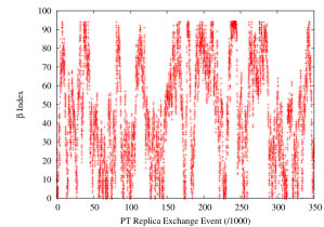
Figure 1: Proper temperature dynamics for one of 95 replicas for $\ell=15$.

IV.1 Parallel tempering efficiency

In the current context, we call the simulation efficient if it generates many independent configurations in an unbiased way in a given simulated time period. For instance, since the PT simulations can be seen as replicas moving from temperature to temperature while they change their configurations, if a certain replica gets stuck in a certain range of temperatures, the sampling would be biased. To obtain good sampling, one should tune the number of used replicas, the temperature difference between successive temperatures $\Delta\beta$, and the duration of the simulated time period between consecutive replica exchange events, the so-called PT update period. These parameters have a strong effect on the efficiency of dynamics. Since decreasing the PT update period may cause the replicas to explore a smaller part of the configurational space, there is an optimum value for this parameter for a fixed computational cost, which has to be found by trial and error. A key concept to assess the efficiency of a PT simulation is a PT cycle, which is the simulated time for the replica to travel between the minimum and maximum temperatures and back.Sheldon:84 For efficient sampling, several cycles should be observed in one run. The value for the PT update period which leads to the largest number of PT cycles is different for various lengths, $\ell$, of the chain under consideration. However, the number of interaction events during each PT update period for 15, 20 and 25 beads chains are similar. This provides a good initial estimate for the optimum value of the PT update period of the larger systems based on the results of smaller systems, and facilitates the trial and error process.

In principle, increasing the number of replicas would make it possible to study any range of temperatures. However, it was found that when the PT system contains a large number of replicas, some of the replicas may not move very well among the full range of temperatures during one PT cycle. This can lead to a prohibitively inefficient PT dynamics. In addition, it was found that the presence of a phase transition in the solvent model reduces the range of temperatures that can be studied (see Sec. IV.2).

As an example, Fig. 1 shows proper dynamics for the 15-bead chain in which the temperature range $T_{l}^{*}=[0.76,2.5]$ is investigated by 95 replicas. For this case the inverse temperature difference $\Delta\beta_{l}^{*}$ for the 10 replicas with the highest temperatures is 0.012 and in the next 60 replicas the $\Delta\beta_{l}^{*}$ decreases linearly to 0.008 and then it remains constant. The PT update period for this case is 0.8 ps. The motivation for using a varying $\Delta\beta$ can be found in I. Plots like the one in Fig. 1 are a helpful tool in checking for poor sampling. The example in Fig. 2 shows what such a plot looks like for a poorly behaving PT simulation in which the temperature range $T_{l}^{*}=[0.82,2.5]$ is investigated using 79 replicas. For this case, the PT update period is 2 ps, which is 2.5 times larger than the previous case in Fig. 1. $\Delta\beta_{l}^{*}$ for the highest 30 temperatures is 0.012, and then for the next 40 temperatures the $\Delta\beta_{l}^{*}$ decreases linearly to $0.008$ and then $\Delta\beta$ remains constant for the rest of temperatures.

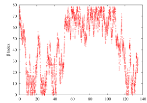
Figure 2: The effect of phase transition, which happens around $\beta$ index 50, on the PT dynamics for one of 79 replicas for $\ell=15$.

(a)                                                                  (b)

 
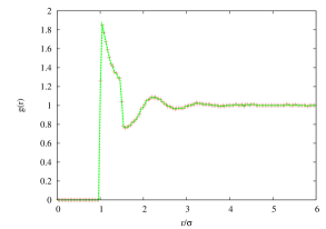
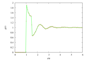
(c)                                                                  (d)

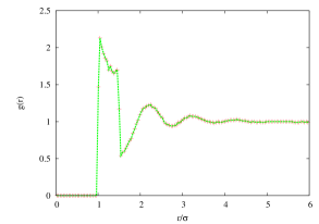
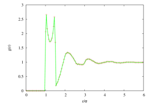
Figure 3: Radial distribution function for the square-well fluid at different temperatures $T_{l}^{*}$: (a) $2.0$, (b) $1.25$, (c) $0.83$, and (d) $0.31$. Lines are drawn to guide the eye.

IV.2 Phase of the solvent

Figure 2 shows an apparent barrier in the PT dynamics at a specific temperature. In other words, replicas have a strong tendency to stay above, or below, that specific temperature, and rarely cross it. While choosing proper parameters that optimize the efficiency of the PT method can improve sampling in the vicinity the temperature barrier, the efficiency of the sampling drops significantly for larger systems (i.e. for $\ell=20$ and $\ell=25$). It turns out that the apparent barrier is related to the phase of the solvent.

The highest temperature in the simulations was $T_{l}^{*}=2.5$ for all chain lengths, while the lowest values for $T_{l}^{*}$ were 0.76, 1.05 and 1.22 for the 15-bead, 20-bead and 25-bead systems, respectively. The square-well model for the solvent has been studied extensivelyErringtonRf3:35 ; OreaRf4:36 ; Schollref5:37 ; Escamillaref6:38 ; Orkoulas:40 ; Elliott:41 ; Rio:42 and for the model used here with $\rho^{*}=0.5$ and $\lambda=\sigma^{\prime}/\sigma=1.5$, the critical reduced temperature, $T_{c}^{*}$, for the solvent is predicted to be 1.2172 ErringtonRf3:35 , 1.210 (in Ornstein-Zernike approximation) Schollref5:37 , 1.3603 (using an analytical equation of state based on a perturbation theory) Schollref5:37 , 1.226 Escamillaref6:38 , 1.2180 Orkoulas:40 , 1.27 Elliott:41 and 1.218 Rio:42 . Most of the previous studies ErringtonRf3:35 ; OreaRf4:36 ; Schollref5:37 ; Vega:43 , predict a vapor-liquid coexistence line to be crossed somewhere between $T_{l}^{*}=1.0$ and $T_{l}^{*}=1.2$ for $\rho^{*}=0.5$ and $\lambda=1.5$. The simulated systems are far from a real thermodynamic system so one expect difficulties in observing this transition. Furthermore, finite-size effects may shift the apparent critical temperature.

As a first check to confirm the fluid-like character of the solvent model, the radial distribution function (RDF) of the solvent was studied for four different temperatures. These are plotted in Fig. 3. Due to the two discontinuities in the solvent interaction potential at $\sigma$ and $\sigma^{\prime}$, respectively, the radial distribution function is relatively high between these two points. For $T_{l}^{*}=2.0$, the RDF graph 3(a) is very similar to what was found for this model in the earlier studies (3rd graph in Fig. 2 in Ref. Escamillaref6:38, ). At this temperature, fluid-like long range correlation can be seen already. The RDF for $T_{l}^{*}=1.25$, Fig. 3(b), and that for $T_{l}^{*}=0.83$, Fig. 3(c), look like those of a typical fluid with more pronounced peaks than the high temperature RDF. At relatively low temperatures of $T^{*}=0.31$, as in Fig. 3(d), the onset of short range structural peaks may be showing itself in the first two peaks, while other peaks show a fluid-like behavior, but there is no clear sign of a phase transition.

RDFs are, however, not a very good indicator of a phase transition. Better indicators are the heat capacity $C_{v}$ and the compressibility $\kappa$, which are second derivatives of the free energy. $C_{v}$ can be measured from the fluctuations in energy, while $\kappa$ can be estimated from fluctuations in local density. For the latter, the system is divided into several boxes and the densities in each box and the standard deviation of the local density are calculated. Numerical estimates for the head capacity and compressibility in the canonical ensemble are plotted in Figs. 4 and 5. The range of studied temperatures was clearly sufficient to observe the effects of a phase transition for smaller systems. This phase transition occurs at a temperature that is very close to the temperatures at which other studies predict the liquid-vapor coexistence line for this density.

Fig. 4 shows that the average heat capacity per solvent particle increases with increasing system size at the phase transition point. This suggests that for infinitely large systems, the heat capacity might diverge at the phase transition. To better understand the phase transition and its order, a further study would be required which lies outside the scope of this paper.

In Fig. 5, the variation of the compressibility vs. temperature shows similar behavior to that observed for the heat capacity. By increasing the system size, the compressibility seems to diverge to infinity around the same point where the heat capacity diverges. This confirms that there is a phase transition at this point.

While these results are for a pure solvent system, our studies revealed that there is no major difference in the behaviors of heat capacity and compressibility for the systems containing the protein-like chain.

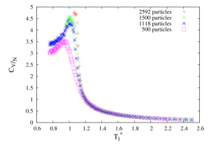
Figure 4: Heat capacity of the square-well solvent per particle vs. the liquid reduced temperature for $N=$ 500, 1118, 1500 and 2592.

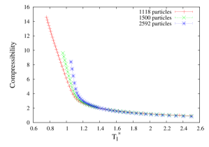
Figure 5: Compressibility of the square-well solvent vs. the liquid reduced temperature for $N=$ 1118, 1500 and 2592.

IV.3 Observed structures and free energy landscape

Simulations using PT and DMD were performed for three different chain lengths: $\ell=15,$ 20 and 25, all in a liquid at density $\rho^{*}=0.5$. The ranges of temperatures and numbers of replicas differed in all these cases. The quantities of interest were the frequencies of occurrence ($f_{\mathrm{obs}}$) of each configuration. The most frequently occurring configuration at any given temperature will be called the dominant configuration if its population is clearly higher than the second most common structure.

All errors reported below indicate the 95% confidence intervals, which is equal to 1.96 times the standard deviation for normally distributed errors. Below, the configurational potential energy only refers to the intra-chain bonds energy, and the term bond refers to a hydrogen bond and not the repulsive interactions, unless otherwise specified.

IV.3.1 15-bead chain

For $\ell=15$, $95$ temperature values were selected for the replicas, such that $\Delta\beta_{l}^{*}=0.012$ for the highest 10 temperatures and then for the next 60 temperatures, the $\Delta\beta_{l}^{*}$ linearly decreases to become $0.008$ at the 70th highest temperature and then $\Delta\beta$ value remains constant for the the rest of temperatures, while the range of studied temperatures is $T^{*}_{l}=[0.76~{},~{}2.5]$ ($\beta^{*}=[1.7~{},~{}5.64]$). The most efficient PT update period was found in the range of 0.8 to 1.2 picoseconds. Below, the value of 0.8 ps was used. These values are smaller than the PT update period used in the solvent-less case of I, which was two picoseconds. As mentioned above, the number of solvent particles appropriate for this case to generate the density of 0.5 is $N=1066$, while the length of the sides of the periodic box is $L=54.4$ Å.

In Table 1, the results for the dominant configuration at different temperatures are presented for the system in the presence and in the absence of any solvent. One sees that at low enough temperature one structure (BF FJ JN) becomes clearly dominant as its probability exceeds 60%.

In Table 2, the population and the average system energies of the most populated structures are provided for $T_{l}^{*}=0.816$ ($\beta^{*}=5.25$), which is a relatively low temperature. The configuration with the lowest configurational potential energy of the system is observed to be the one with the lowest total potential energy. One also sees that the next three populated structures in Table 2 have very close values for $f_{\mathrm{obs}}$ and for the average total potential energy of the system.

In terms of the free energy landscape, one can interpret these results as follows. The landscape consists of a relatively deep global minimum at BF FJ JN, which has three local free energy minima (BF FJ, BF JN, and FJ JN) close to it, since these configurations differ by only one bond from the first configuration. Since the last three configurations in Table 2 also differ by only two bonds from the first configuration, their locations in the landscape should be further from the deepest point such that the configurations 2,3 and 4 should be located between the deepest point and these configurations. A rough picture of this landscape is presented in Fig. 6 in which the distances between the structures are based on their similarities and the area differences are related to the differences in their computed entropy in the absence of the solvent (see I). The lowest free energy structure at low temperatures, BF FJ JN, has been located in the middle, and the other structures are positioned based on their similarities to the BF FJ JN configuration. For example, BF FJ is located between the deepest point (BF FJ JN) and BF and FJ. This diagram gives some idea about the folding pathways. For example, to reach the lowest energy structure with three bonds from the structure with no bonds, initially, the first bond and then the second bond should be made, which could occur along six different pathways.

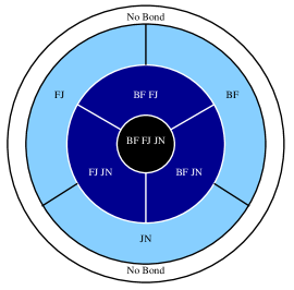
Figure 6: A qualitative picture of the 15-bead chain landscape.

According to Table 2, the lowest potential energy configuration, BF FJ JN, is associated with the lowest total potential energy of the system as well. However, since the uncertainty in the computed energies of the 7th structure in Table 2 is relatively large, the data in the table is not sufficient to conclude that the configuration with the lowest total potential energy is BF FJ JN. However, there are good arguments for why the first configuration should have the lowest total potential energy. The first configuration is the most populated one for all the 66 temperatures that lie in $T^{*}_{l}=[0.76~{},~{}2.0]$, so it is the lowest free energy system at these temperatures. By adding more bonds and consequently adding more geometrical restrictions, the configurational entropy decreases, and therefore BF FJ JN has the lowest configurational entropy among 15-bead configurations. Under the assumption that the average entropy contributions from the solvent particles for different configurations are very similar, one can conclude that the BF FJ JN configuration should have the lowest total potential energy for $T^{*}_{l}=[0.76~{},~{}2.0]$. It is expected that for the short chains, where the chains do not collapse, the potential energy difference between two systems mainly depends on their configurational potential energy difference, while the average potential energy contribution from the solvent particles will be roughly the same for different systems energies. To illustrate this, for example, at $\beta^{*}=5.25$ ($T_{l}^{*}=0.816$) BF FJ JN and BF JN, the two most populated configurations of Table 2, have on average $0.1\pm 0.02$ and $0.19\pm 0.3$ bonds with solvent particles, respectively. Hence, the contribution to the total potential energy difference from the bonds between solvent particles and the chain beads is around 0.02 $\epsilon$, while their configurational potential energy difference is $1\epsilon$. The average number of bonds that each solvent particle makes with other solvent particles at $\beta^{*}=5.25$ ($T_{l}^{*}=0.816$) is around 5.1.

${\beta^{*}}$	in solvent	$f_{\rm obs}$(%)	solventless	$f_{\rm obs}$(%)
1.8	No bond	18.2 $\pm$ 0.8	No bond	41.3 $\pm$ 1.5
2.4	No bond	18.9 $\pm$0.6	No bond	30.15 $\pm$ 1.6
3.0	No bond	11.3 $\pm$ 0.8	No bond	19.7 $\pm$ 1.3
3.6	BF FJ JN	24.0 $\pm$ 0.9	BF JN	17.1 $\pm$ 1.2
4.2	BF FJ JN	37.7 $\pm$ 0.8	BF FJ JN	26.7 $\pm$ 1.5
4.5	BF FJ JN	43.2 $\pm$ 0.9	BF FJ JN	35.0 $\pm$ 1.5
4.8	BF FJ JN	53.3 $\pm$ 0.8	BF FJ JN	44.1 $\pm$ 1.6
5.1	BF FJ JN	60.5 $\pm$ 1.2	BF FJ JN	55.1$\pm$ 1.8
5.4	BF FJ JN	67.3 $\pm$ 0.9	BF FJ JN	61.5 $\pm$ 1.6
9	N/A	N/A	BF FJ JN	98.6 $\pm$ 0.4

Table 1: Most common configurations of the 15-bead chain for different temperatures, with and without the solvent.

rank	configuration	$f_{\rm obs}$(%)	potential energy
			total/$\epsilon$	chain/$\epsilon$
1	BF FJ JN	64.9 $\pm$ 0.9	-1273.3 $\pm$ 0.3	-3
2	BF JN	10.9 $\pm$ 0.5	-1271.7 $\pm$ 0.7	-2
3	FJ JN	9.6 $\pm$ 0.5	-1272.0 $\pm$ 0.7	-2
4	BF FJ	8.9 $\pm$ 0.5	-1271.8 $\pm$ 0.7	-2
5	JN	1.5 $\pm$ 0.1	-1271.9$\pm$ 1.8	-1
6	FJ	1.5 $\pm$ 0.1	-1272.1 $\pm$ 1.9	-1
7	BF	1.3 $\pm$ 0.1	-1272.6 $\pm$ 1.8	-1

Table 2: Most populated configurations and their energies of the 15-bead chain with the solvent environment at $T_{l}^{*}=0.816(\beta^{*}=5.25$).

If BF FJ JN has the lowest potential energy of the system, one expects that the population of this configuration will approach 100% at lower temperatures where the free energy mainly depends on the total potential energy of the system and little on the system entropy. This trend of the population was indeed seen in the solventless case in I for chains smaller than 30 beads. The population of the 15-bead dominant structure both with and without the solvent, are compared in Fig. 7, where in both cases (with and without a solvent) the probability of the dominant structure reaches a high value. This behavior happens at higher temperatures inside the solvent, which suggests that the hydrophobic effects of 75% of the chain beads assist the folding process and make the helical structures more favorable. Another consequence of the hydrophobicity is that at all temperatures, the average radius of gyration for the 15-bead chain inside the solvent was found to be smaller than in the absence of the solvent, which shows that the fluid is a poor solvent.

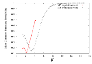
Figure 7: The probability of the most common structure versus inverse temperature $\beta^{*}$ for the 15-bead chain with and without the solvent.

IV.3.2 20-bead chain

Generally, it is harder to study a wider range of temperatures for large systems due to the need to use smaller $\Delta\beta$ and consequently, a higher number of replicas (while each system also contains more particles). However, as was discussed in section IV.1, for the case of a chain in a square-well solvent, simulating a wide range of temperatures becomes extremely hard due to the effect of the phase transition on the PT dynamics. Consequently, for $\ell=20$, the range of studied temperatures, from $T_{l}^{*}=1.05$ to $2.5$ ($\beta^{*}=[1.7~{},~{}4.1]$), is smaller than it was for $\ell=15$. To study the energy landscape, 79 temperature values were selected for the replicas such that $\Delta\beta_{l}^{*}=0.008$ for the 40 highest temperatures and then $\Delta\beta_{l}^{*}$ decreases to 0.006 and remains constant for the the rest of temperatures. For $\ell=20$, the number of appropriate solvent particles to generate a density of 0.5 for the system with the periodic box of $L=72$ Å is $N=2522$. The most efficient PT update period was found to be 320 femtoseconds, which is smaller than the value of 15-bead case. While it was found that 320 femtoseconds is the most efficient value for the PT update period of the 20-bead chain system, there is a range, 260–320 femtoseconds, that yields similar efficiencies. As mentioned above, around $T_{l}^{*}=1.1$, the heat capacity and compressibility of the fluid show signs of a phase transition, in line with other studies that predict the location of the vapor-liquid coexistence line. Because of the phase transition, trying to reach lower temperatures resulted in poor dynamics even when using small values for $\Delta\beta^{*}$, so the lowest temperature was kept at $T^{*}_{l}=1.05$.

The dominant configurations at different temperatures in the presence and in the absence of the solvent are presented in Table 3. The effective lower limit on reachable temperatures imposed by the phase transition in the solvent, made it impossible to determine whether the probability of the most populated structure approaches one at lower temperatures. Table 4 shows that at $\beta^{*}=3.9$, BF FJ JN NR is the most populated structure while BF BR FJ JN NR, which has the lowest configurational potential energy, has a smaller population. BF FJ JN NR, is a complete helical structure because it has all the necessary helical bonds between every two consecutive turns of the protein-like chain; while BF BR FJ JN NR, the lowest potential energy configuration, is a collapsed helical structure with an additional bond BR that connects the two ends of the chain. Hence, BF FJ JN NR, an unfolded but completely helical structure, has a much higher entropy than the lowest potential energy configuration, while their energies are close since they only differ by one internal bond. Furthermore, the complete helical structure can make more bonds with the solvent particles because of its non-collapsed shape, as evidenced by the fact that 17% of the population of the complete helical structure make bonds with the solvent particles at $\beta^{*}=3.9$ ($T_{l}^{*}=1.1$), while only 4% of the lowest potential energy configuration population make such bonds. The number of bonds with the solvent particles also shows that in this model the structures are not soluble, and the potential energy contribution from bonds between the chain beads and the solvent particles to the potential energy of the system is relatively small.

${\beta^{*}}$	in solvent	$f_{\rm obs}$(%)	solventless	$f_{\rm obs}$(%)
1.8	No bond	7.2 $\pm$ 0.5	No bond	28.3 $\pm$ 1.6
2.4	No bond	7.8 $\pm$ 0.5	No bond	21.5 $\pm$ 1.3
3.0	No bond	4.6 $\pm$ 0.4	No bond	11.6 $\pm$ 1.1
3.3	BF FJ JN NR	6.5 $\pm$ 0.5	BF	7.3 $\pm$ 0.9
3.6	BF FJ JN NR	10.3 $\pm$ 0.6	BF NR	7.6 $\pm$ 0.8
3.9	BF FJ JN NR	12.3 $\pm$ 0.6	BF JN NR	9.8 $\pm$ 0.8
4.5	N/A	N/A	BF FJ JN NR	16.3 $\pm$ 1.3
6.0	N/A	N/A	BF BR FJ JN NR	47.7 $\pm$ 1.6
10.5	N/A	N/A	BF BR FJ JN NR	99.1 $\pm$ 0.3

Table 3: Most populated configurations of the 20-bead chain inside and in the absence of the solvent.

According to Table 4, the total potential energies of the most populated structures are very close to each other. It is therefore hard to predict whether there is a dominant structure at lower temperatures, as seen in the solvent-less 20-bead chain.hanif:34 While the non-collapsed helical structure can make more bonds with solvent particles in comparison with the lowest potential energy configuration, the average number of bonds with the solvent particles is still less than one. It is expected that the average potential energy contribution from the bonds between solvent particles is very similar for different configurations. However, it would require much better sampling statistics than what was obtained to check this prediction. Since the potential energy of each intra-chain bond is equivalent to 4.29 bead-solvent bonds, it is expected that the configuration with the lowest configurational potential should have the lowest total potential energy as well, and should, therefore, become the most common structure at lower temperatures. The reason that the lowest potential energy configuration does not become dominant at the studied temperatures is that the BR bond greatly restricts the configurational freedom and therefore, the non-collapsed helical structure, having one less bond but with much larger entropy, becomes the most common structure.

Apart from the potential energies and populations of the different configurations, one can also get an idea of their relative configurational entropies, although not as precise as in I. The population of the the lowest potential energy configuration with the largest number of bonds becomes equal to that of the structure with no potential energy (no bond) at $\beta^{*}\approx 3.27$, while this happens at lower temperature, $\beta^{*}\approx 4.05$, in the absence of a solvent. At $\beta^{*}=3.27$ in the solvent environment, only 15% of the lowest potential energy configurations make bonds with the solvent particles, while 89% structures without internal bonds, make bonds with the solvent particles. By assuming that the potential energy contribution from bonds between solvent particles is almost the same for these two configurations, and since they differ by 5 bead-bead bonds, it can be concluded that the difference in the average potential energy of the system in this case is likely about $5\epsilon$ (perhaps somewhat less). The populations of two structures become equal when their free energy difference is around zero. Therefore, the entropy difference of the no bond structure and the lowest potential energy configuration, $\Delta S$, can be calculated as $\Delta S=5\varepsilon/T=5k_{B}\beta^{*}$. According to this calculation, in the absence of the solvent $\Delta S\simeq 20.25k_{b}$ and in the solvent environment $\Delta S\leq 16.35k_{b}$. Since these two configurations are the least and the most restricted ones, respectively, $\Delta S$ represents the maximum configurational entropy difference. Hence, having a hydrophobic chains in this model results in a smaller entropy range, which indicates that in comparison with the previous work in the absence of a solvent, the probability of the dominant configuration would approach one at higher temperatures, just as we saw in the previous case of the 15-bead chain, cf. Fig. 7.

rank	configuration	$f_{\rm obs}$(%)	potential energy
			total/$\epsilon$	chain/$\epsilon$
1	BF FJ JN NR	12.3 $\pm$ 0.6	-2482.6 $\pm$ 1.4	-4
2	BF FJ NR	8.5 $\pm$ 0.4	-2484.4 $\pm$ 1.6	-3
3	BF JN NR	8.2 $\pm$ 0.4	-2483.1 $\pm$ 1.6	-3
4	BF FJ JN	7.3 $\pm$ 0.5	-2482.6 $\pm$ 1.8	-3
5	FJ JN NR	7.3 $\pm$ 0.5	-2482.7 $\pm$ 1.8	-3
6	BF BR FJ JN NR	5.3 $\pm$ 0.4	-2483.6 $\pm$ 2.2	-5
7	BF JN	4.6 $\pm$ 0.4	-2484.1 $\pm$ 2.2	-2

Table 4: Most populated configurations of the 20-bead chain inside the solvent at $\beta^{*}=3.9$ ($T_{l}^{*}=1.1$).

IV.3.3 25-bead chain

For the 25-bead chain, the system needs to include 4644 solvent particles, which is nearly twice the number of solvent particles as in the 20-bead system, in a box of $L=88$ Å. According to Fig. 4, the temperature at which the phase transition behavior is observed increases slightly with increasing $N$. Therefore, the range of temperatures that could be investigated for the 25-bead chain system is even smaller than 20-bead case. A set of temperatures with 95 replicas was chosen, such that for the 20 highest temperatures $\Delta\beta=0.006$, and for the rest of temperatures $\Delta\beta=0.004$, while the range of studied temperatures is $T^{*}_{l}=[1.22~{},~{}2.5]$ ($\beta^{*}=[1.7~{},~{}3.5]$). The most efficient PT update period is 120 femtoseconds, which is even smaller than in the 20-bead case.

According to Table 5, the structure with the lowest configurational potential energy becomes dominant at higher temperatures in comparison with the solvent-less case of I. However, the range of studied temperature is not sufficient to observe the kind of deep funnel in the free energy landscape at low temperatures that was observed in the absence of a solvent. The most common structures of the 25-bead chain inside a solvent at $\beta^{*}=3.3$ are presented in Table 6. While the populations of configurations 3-10 are equal within the statistical error, the population of the first configuration (with 8 bonds) is clearly higher than that of the other configurations. Our study reveals that this configuration is clearly the most populated one for $T_{l}^{*}\leq 1.32$ ($\beta^{*}\geq 3.24$). This means that for all the temperatures in the range $1.22\leq T_{l}^{*}\leq 1.32$ ($3.24\geq\beta^{*}\geq 3.0$), the structure with the lowest configurational potential energy is the most common structure. Since the configurational entropy decreases by increasing the number of bonds (because of adding more restrictions), the first configuration should have the lowest configurational entropy. Since the first configuration has been the most common structure at the lowest studied temperature, the system containing the first configuration should be the lowest total potential energy at these temperatures. It is expected that by decreasing the temperature, the order of the system energies does not change dramatically and therefore, when decreasing the temperature, the first configuration likely remains the one with the lowest total potential energy and therefore, the population of this structure should approach one at low temperatures, similar to the results of I.

For the 25-bead case, a similar reasoning as for the 20-bead chain leads to the prediction of a large configurational entropy difference between the lowest potential energy configuration with a completely collapsed shape (first configuration of Table 6) and the non-collapsed helical structure (second configuration of Table 6). Therefore, one anticipates that the non-collapsed helical structure has the highest occupancy for the limited range of temperatures that was studied in the simulations. However, because of the potential energy difference of 3$\epsilon$, the first configuration becomes dominant, even at not very low temperatures. This is unlike the 20-bead chain, for which the non-collapsed helical structure (1st configuration of Table 4) is dominant at similar temperatures. Consequently, the probability of the collapsed helical structure of the 25-bead chain approaches one at lower temperatures as it does in the absence of the solvent.

${\beta^{*}}$	in solvent	$f_{\rm obs}$(%)	solventless	$f_{\rm obs}$(%)
1.8	No bond	2.7 $\pm$ 0.3	No bond	21.7 $\pm$ 1.3
2.4	No bond	3.3 $\pm$ 0.3	No bond	15.5$\pm$ 1.0
3.0	NR	1.3 $\pm$ 0.2	No bond	6.7 $\pm$ 0.9
3.3	BF BR BV FJ FV JN NR RV	2.6 $\pm$ 0.2	No bond	4.3 $\pm$ 0.6
4.5	N/A	N/A	BF BR BV FJ FV JN NR RV	7.5 $\pm$ 1.0
9.0	N/A	N/A	BF BR BV FJ FV JN NR RV	98.0 $\pm$ 0.4

Table 5: Most populated configurations of the 25-bead chain inside and in the absence of the solvent.

rank	configuration	$f_{\rm obs}$(%)	potential energy
			total	chain
1	BF BR BV FJ FV JN NR RV	3.4 $\pm$ 0.3	-4219.9 $\pm 1.9$	-8
2	BF FJ JN NR RV	2.0 $\pm$ 0.3	-4217.7 $\pm$ 2.5	-5
3	FJ JN NR RV	1.5 $\pm$ 0.2	-4216.0 $\pm$ 2.7	-4
4	BF FJ JN NR	1.5 $\pm$ 0.3	-4219.4 $\pm$ 2.9	-4
5	BF FJ JN RV	1.5 $\pm$ 0.3	-4215.8 $\pm$ 3.0	-4
6	BF BR BV FJ JN NR RV	1.3 $\pm$ 0.2	-4218.4 $\pm$ 2.9	-7
7	BF FJ NR RV	1.3 $\pm$ 0.2	-4215.2 $\pm$ 3.0	-4
8	BF JN NR	1.3 $\pm$ 0.1	-4213.0 $\pm$ 3.7	-3
9	JN NR RV	1.2 $\pm$ 0.1	-4216.3 $\pm$ 2.9	-3
10	FJ JN RV	1.2 $\pm$ 0.1	-4213.1 $\pm$ 3.1	-3

Table 6: Most populated configurations of the 25-bead chain inside the solvent at $\beta^{*}=3.3$ ($T_{l}^{*}=1.30$).

V Conclusions

The free energies of different configurations (i.e., the free energy landscape) of a protein-like chain in a solvent at different temperatures were investigated. Qualitatively, the behavior of a protein-like chain inside a square-well solvent is similar to the behavior in the absence of a solvent, studied in I. For the 15-bead chain, the lowest free energy configuration was found to be an alpha helix that becomes dominant at low temperatures, just as it did in the absence of any solvent. The free energy landscape of the 15-bead chain at low temperatures consists of a funnel with a very deep global minimum and a few local minima around it. By lowering the temperature, the global minimum becomes deeper while the others become shallower and consequently, the funnel becomes steeper.

For larger chain lengths, in particular, for $\ell=20$ and $\ell=25$, a phase transition of the square-well solvent effectively puts a lower bound on the temperature range accessible in the simulations. The observed phase transition temperature coincides roughly with the temperature at which previous studies observed a liquid-vapor coexistence line. Investigating the free energy landscape of a solvated system over a phase transition point of the solvent can be very challenging using the PT method, especially for larger systems. For the 20-bead and 25-bead chains the effects of the phase transition become more apparent because of the larger number of particles in comparison with the 15-bead chain. Consequently, the temperature range studied here could not be extended below the (effective) phase transition temperature for the 20-bead and 25-bead chains. This difficulty is not easy to overcome, since it is related to the efficiency of the PT algorithm itself near the phase transition point. Substantial computational resources, over a million cpu hours, were used to obtain the results presented here, which were mainly utilized to obtain the best set of parameters for the PT runs. As a result of the considerable computational demand of computing the free energy of the solvated system below the phase transition point, a direct comparison for the 20-bead and 25-bead chain systems with the previous study could not be done for the whole range of temperatures that were investigated in I. However, it is expected that for both 20-bead and 25-bead chain systems the configuration with the lowest configurational energy becomes dominant at lower temperatures, since their systems energy seem to be the lowest ones at very low temperatures, which is mainly due to their low configurational energy and the hydrophobicity of 75% of protein-like chain beads (having only hard-core repulsive interactions with solvent particles).

While for the 15-bead chain the lowest potential energy configuration is an unfolded alpha-helix without any specific tertiary structure, for longer chains, the bonds between different layers of the helix, such as the bond between two ends of the chain, cause the lowest potential energy structure to be a folded structure. Our study showed that the entropic barrier for making bonds between the two ends of the chain for longer chains is larger than the change in entropy associated with forming a helix structure. As a consequence, the unfolded helical structure is dominant for a relatively large range of temperature until the low-temperature regime where the folded helix is favored. Therefore, similar to the absence of a solvent, the effect of temperature on the morphology of the landscape is more apparent for the longer chains.

One of the major differences between a protein model in a solvent (studied here) and without a solvent (studied in I) is the effect of mainly repulsive interactions of the beads with the solvent particles in the folding process. Only 25% of the beads can make attractive bonds with the solvent, while the rest of the beads only have repulsive interactions with the solvent (i.e., they are hydrophobic). Because of the restriction effects of the repulsive interactions, the entropy range (i.e., the entropy difference of the minimum and maximum number of bonds configurations) is smaller in comparison with the absence of a solvent. Because of the smaller entropy range, the landscape shows funnel behavior at higher temperatures in comparison with the absence of a solvent.

The main problem in studying the protein-like chain inside the solvent is the slow convergence of estimates of the free energy of configurations using the PT method. For example, the presence of a phase transition in the square-well fluids leads to large statistical errors in the PT method. To overcome the effects of the phase transition on sampling, the PT method should be enhanced by incorporating other techniques, such as the umbrella sampling.Valleau:48 Another solution for this problem is to use different parameters for the square-well liquid, such that the phase transition temperature lies outside the temperature range of interest. According to Ref. OreaRf4:36, , by increasing the ratio $\lambda=\sigma^{\prime}/\sigma$, the liquid-vapor coexistence line shifts to higher temperatures for the density of $\rho^{*}=0.5$. For example, for $\lambda=2.0$ the liquid-vapor coexistence line is crossed at a temperature around $T_{l}^{*}=2.4$ for $\rho^{*}=0.5$,OreaRf4:36 ; ErringtonRf3:35 ; Miguel:49 which is very close to the highest studied temperature ($T_{l}^{*}=2.5$). While using $\lambda\geq 2$ can be helpful for avoiding the phase transition, it would allow for an unphysically large range of bond vibrations in comparison with real proteins.

One of the possible avenues for future research is to investigate the dynamics of the folding transition, instead of only the resulting free energies. While studying the folding pathways can be computationally very demanding, it provides more information about the nature of folding. Some earlier studies have provided some simple connections between energy landscapes and protein folding kinetics, which can be applied (under suitable assumptions) to this study.Szabo:77 ; Hamm:78 For example, by considering the distance between any two beads that can make a bond as a reaction coordinate, it is possible to observe the potential of mean force (Helmholtz free energy) versus the reaction coordinate (distance of the two beads that can make a bond). From this potential of mean force, one can estimate first passage times (Kramers’ problem) to extract rates of forming and breaking a bond. These rate enter the relaxation matrix in a rate equation approach, which could then be used to analyze to the dynamics of protein folding.

- (1) E. Shakhnovich, Chem. Rev. 106, 1559 (2006).
- (2) Editorial, Science 309, 78 (2005).
- (3) C. Levinthal, J. Chim. Phys. 65, 44–45 (1968).
- (4) J. D. Bryngelson, J. N. Onuchic, N. D. Socci, and P. G. Wolynes, Proteins:Struct. Funct. Genet. 21, 167–195 (1995).
- (5) S. Govindarajan and R. A. Goldstein, Proc. Natl. Acad. Sci. USA 95, 5545–5549 (1998).
- (6) A. Schug, T. Herges, A. Verma, and W. Wenzel, J. Phys.: Condens. Matter 17, S1641 (2005).
- (7) C. Anfinsen, Science 181, 223 (1973).
- (8) D. N. Woolfson, A. Cooper, M. M. Harding, D. H. Williams, and P. A. Evans, J. Mol. Biol. 229, 502 (1993).
- (9) M. V. Athawale, G. Goel, T. Ghosh, T. M. Truskett, and S. Garde, Proc. Natl. Acad. Sci. USA 104, 733 (2007).
- (10) S. Rajamani, T. M. Truskett, and S. Garde, Proc. Natl. Acad. Sci. USA 102, 9475 (2005).
- (11) V. Soundararajan, R. Raman, S. Raguram, V. Sasisekharan, and R. Sasisekharan, PLoS ONE 5, e9391 (2010).
- (12) Y. M. Rhee, E. J. Sorin, G. Jayachandran, E. Lindahl, and V. S. Pande, Proc. Natl. Acad. Sci. USA 101, 6456 (2004).
- (13) H. Bayat-Movahed, R. van Zon, and J. Schofield (2011), arXiv:1108:2912.
- (14) R. H. Swendsen and J.-S. Wang, Phys. Rev. Lett. 57, 2607 (1986).
- (15) C. J. Geyer, in Proceedings of the 23rd Symposium on the Interface: Computing Science and Statistics (1991), pp. 156–163.
- (16) M. C. Tesi, E. J. J. van Rensburg, E. Orlandini, and S. G. Whittington, J. Stat. Phys. 82, 155 (1996).
- (17) D. J. Earl and M. W. Deem, Phys. Chem. Chem. Phys., 7, 3910 (2005).
- (18) A. Bellemans, J. Orban, and D. van Belle, Mol. Phys. 39, 781 (1980).
- (19) J. K. Singh, D. A. Kofke, and J. R. Errington, J. Chem. Phys. 119, 3405 (2003).
- (20) P. Orea, Y. Duda, V. C. Weiss, W. Schröer, and J. Alejandre, J. Chem. Phys. 120, 11754 (2004).
- (21) E. Schöll-Paschinger, A. L. Benavides, and R. Castañeda-Priego, J. Chem. Phys. 123, 234513 (2005).
- (22) I. Guillén-Escamilla, M. Chávez-Páez, and R. Castañeda-Priego, J. Phys.: Condens. Matter 19, 086224 (2007).
- (23) G. Orkoulas and A. Z. Panagiotopoulos, J. Chem. Phys. 110, 1581 (1999).
- (24) J. R. Elliott and L. Hu, J. Chem. Phys. 110, 3043 (1999).
- (25) F. D. Rio, E. Avalos, R. Espindola, L. F. Rull, G. Jackson, and S. Lago, Mol. Phys. 100, 2531 (2002).
- (26) L. Vega, E. de Miguel, L. F. Rull, G. Jackson, and I. A. McLure, J. Chem. Phys. 96, 2296 (1992).
- (27) A. Lang, G. Kahl, C. N. Likos, H. Löwen, and M. Watzlawek, J. Phys.: Condens. Matter 11, 10143–10161 (1999).
- (28) N. D. Socci, J. N. Onuchic, and P. G. Wolynes, Proteins 32, 136 (1998).
- (29) H. Frauenfelder, F. Parak, and R. D. Young, Annu. Rev. Biophys. Biophys. Chem. 17, 451 (1988).
- (30) D. C. Rapaport, The art of molecular dynamics simulation (Cambridge University Press, Cambridge, 2004), 2nd ed.
- (31) L. Hernández de la Peña, R. van Zon, J. Schofield, and S. B. Opps, J. Chem. Phys. 126, 074105 (2007).
- (32) S. Duane, A. D. Kennedy, B. J. Pendleton, and D. Roweth, Phys. Lett. B 195, 216 (1987).
- (33) W. Gropp, E. Lusk, and A. Skjellum, Using MPI: Portable Parallel Programming with the Message-Passing Interface (MIT Press, Cambridge, MA, 1994).
- (34) S. B. Opps and J. Schofield, Physical Review E 63, 056701 (2001).
- (35) G. M. Torrie and J. P. Valleau, Journal of Computational Physics 23, 187 (1977).
- (36) E. de Miguel, Phys. Rev. E 55, 1347–1354 (1997).
- (37) D. J. Bicout and A. Szabo, Protein Sci. 9, 452–465 (2000).
- (38) P. Hamm, J. Helbinga, and J. Bredenbecka, Nonequilibrium Dynamics in Biomolecules 323, 54 (2006).