Hitting distributions of $\alpha$-stable processes via path censoring and self-similarity

Abstract

We consider two first passage problems for stable processes, not necessarily symmetric, in one dimension. We make use of a novel method of path censoring in order to deduce explicit formulas for hitting probabilities, hitting distributions, and a killed potential measure. To do this, we describe in full detail the Wiener-Hopf factorisation of a new Lamperti-stable-type Lévy process obtained via the Lamperti transform, in the style of recent work in this area.

Key words and phrases: Lévy processes, stable processes, hitting distributions, hitting probabilities, killed potential, stable processes conditioned to stay positive, positive self-similar Markov processes, Lamperti transform, Lamperti-stable processes, hypergeometric Lévy processes.

MSC 2010 subject classifications: 60G52, 60G18, 60G51

1 Introduction

A Lévy process is a stochastic process issued from the origin with stationary and independent increments and càdlàg paths. If $X:=(X_{t})_{t\geq 0}$ is a one-dimensional Lévy process with law $\mathrm{P}$, then the classical Lévy-Khintchine formula states that for all $t\geq 0$ and $\theta\in\mathbb{R}$, the characteristic exponent $\Psi(\theta):=-t^{-1}\log\mathrm{E}(e^{\mathrm{i}\theta X_{t}})$ satisfies

$$\Psi(\theta)=\mathrm{i}a\theta+\frac{1}{2}\sigma^{2}\theta^{2}+\int_{\mathbb{R}}(1-e^{\mathrm{i}\theta x}+\mathrm{i}\theta x\mathbbm{1}_{(|x|\leq 1)})\Pi(\mathrm{d}x),$$

where $a\in\mathbb{R}$, $\sigma\geq 0$ and $\Pi$ is a measure (the Lévy measure) concentrated on $\mathbb{R}\setminus\{0\}$ such that $\int_{\mathbb{R}}(1\wedge x^{2})\Pi(\mathrm{d}x)<\infty$.

$(X,\mathrm{P})$ is said to be a (strictly) $\alpha$-stable process if it is a Lévy process which also satisfies the scaling property: under $\mathrm{P}$, for every $c>0$, the process $(cX_{tc^{-\alpha}})_{t\geq 0}$ has the same law as $X$. It is known that $\alpha\in(0,2]$, and the case $\alpha=2$ corresponds to Brownian motion, which we exclude. The Lévy-Khintchine representation of such a process is as follows: $\sigma=0$, and $\Pi$ is absolutely continuous with density given by

$$c_{+}x^{-(\alpha+1)}\mathbbm{1}_{(x>0)}+c_{-}\left\lvert x\right\rvert^{-(\alpha+1)}\mathbbm{1}_{(x<0)},\qquad x\in\mathbb{R},$$

where $c_{+},c_{-}\geq 0$, and $c_{+}=c_{-}$ when $\alpha=1$. It holds that $a=(c_{+}-c_{-})/(\alpha-1)$ when $\alpha\neq 1$, and we specify that $a=0$ when $\alpha=1$; the latter condition is a restriction which ensures that $X$ is a symmetric process when $\alpha=1$, so the only $1$-stable process we consider is the symmetric Cauchy process.

These choices mean that, up to a multiplicative constant $c>0$, $X$ has the canonical characteristic exponent

$$\Psi(\theta)=\begin{cases}c\left\lvert\theta\right\rvert^{\alpha}(1-\mathrm{i}\beta\tan\frac{\pi\alpha}{2}\operatorname{sgn}\theta)&\alpha\in(0,2)\setminus\{1\},\\ c\left\lvert\theta\right\rvert&\alpha=1,\end{cases}\qquad\theta\in\mathbb{R},$$

where $\beta=(c_{+}-c_{-})/(c_{+}+c_{-})$. For more details, see Sato.

For consistency with the literature we appeal to in this article, we shall always parameterise our $\alpha$-stable process such that

$$c_{+}=\frac{\Gamma(\alpha+1)}{\Gamma(\alpha\rho)\Gamma(1-\alpha\rho)}\quad\text{and}\quad c_{-}=\frac{\Gamma(\alpha+1)}{\Gamma(\alpha\hat{\rho})\Gamma(1-\alpha\hat{\rho})},$$

where $\rho=\mathrm{P}(X_{t}\geq 0)=\mathrm{P}(X_{t}>0)$ is the positivity parameter, and $\hat{\rho}=1-\rho$.

We take the point of view that the class of stable processes, with this normalisation, is parameterised by $\alpha$ and $\rho$; the reader will note that all the quantities above can be written in terms of these parameters. We shall restrict ourselves a little further within this class by excluding the possibility of having only one-sided jumps. Together with our assumption about the case $\alpha=1$, this gives us the following set of admissible parameters: rCl A&= { (α,ρ) : α∈(0,1),   ρ∈(0,1) }
∪{ (α,ρ) : α∈(1,2),   ρ∈(1-1/α, 1/α) } ∪{ (α, ρ) = (1, 1/2) }.

After Brownian motion, $\alpha$-stable processes are often considered an exemplary family of processes for which many aspects of the general theory of Lévy processes can be illustrated in closed form. First passage problems, which are relatively straightforward to handle in the case of Brownian motion, become much harder in the setting of a general Lévy process on account of the inclusion of jumps. A collection of articles through the 1960s and early 1970s, appealing largely to potential analytic methods for general Markov processes, were relatively successful in handling a number of first passage problems, in particular for symmetric $\alpha$-stable processes in one or more dimensions. See, for example, [BGR-st-hit, Get1, Get2, Por-htpr, Rog71] to name but a few.

However, following this cluster of activity, several decades have passed since new results on these problems have appeared. The last few years have seen a number of new, explicit first passage identities for one-dimensional $\alpha$-stable processes, thanks to a better understanding of the intimate relationship between the aforesaid processes and positive self-similar Markov processes. See, for example, [CC06, CPP-bernoulli, ChaKypPar09, JCKuz, n-tuple].

In this paper we return to the work of BGR-st-hit, published in 1961, which gave the law of the position of first entry of a symmetric $\alpha$-stable process into the unit ball. Specifically, we are interested in establishing the same law, but now for all the one-dimensional $\alpha$-stable processes which fall within the parameter regime $\mathcal{A}$; we remark that Por-htpr found this law for processes with one-sided jumps, which justifies our exclusion of these processes in this work. Our method is modern in the sense that we appeal to the relationship of $\alpha$-stable processes with certain positive self-similar Markov processes. However, there are two notable additional innovations. First, we make use of a type of path censoring. Second, we are able to describe in explicit analytical detail a non-trivial Wiener-Hopf factorisation of an auxiliary Lévy process from which the desired solution can be sourced. Moreover, as a consequence of this approach, we are able to deliver a number of additional, related identities in explicit form for $\alpha$-stable processes.

We now state the main results of the paper. Let $\mathrm{P}_{x}$ refer to the law of $X+x$ under $\mathrm{P}$, for each $x\in\mathbb{R}$. We introduce the first hitting time of the interval $(-1,1)$,

$$\tau_{-1}^{1}=\inf\{t>0:X_{t}\in(-1,1)\}.$$

Note that, for $x\neq-1,1$, $X_{\tau_{-1}^{1}}\in(-1,1)$ $\mathrm{P}_{x}$-a.s. so long as $X$ is not spectrally one-sided. However, in Proposition 1.3, we will consider a spectrally negative $\alpha$-stable process, for which $X_{\tau_{-1}^{1}}$ may take the value $-1$ with positive probability.

Theorem 1.1.

Let $x>1$. Then, when $\alpha\in(0,1]$,

$$\mathrm{P}_{x}(X_{\tau_{-1}^{1}}\in\mathrm{d}y,\,\tau_{-1}^{1}<\infty)/\mathrm{d}y=\frac{\sin(\pi\alpha\hat{\rho})}{\pi}(x+1)^{\alpha\rho}(x-1)^{\alpha\hat{\rho}}(1+y)^{-\alpha\rho}(1-y)^{-\alpha\hat{\rho}}(x-y)^{-1},$$

for $y\in(-1,1)$. When $\alpha\in(1,2)$, rCl P_x(X_τ_-1^1 ∈dy)/dy &= sin(πα^ρ)π (x+1)^αρ (x-1)^α^ρ (1+y)^-αρ (1-y)^-α^ρ (x-y)^-1
- (α-1) sin(πα^ρ)π (1+y)^-αρ (1-y)^-α^ρ ∫_1^x (t-1)^α^ρ-1 (t+1)^αρ-1  dt, for $y\in(-1,1)$.

When $X$ is symmetric, Theorem 1.1 reduces immediately to Theorems B and C of [BGR-st-hit]. Moreover, the following hitting probability can be obtained.

Corollary 1.2.

When $\alpha\in(0,1)$, for $x>1$,

$$\mathrm{P}_{x}(\tau_{-1}^{1}=\infty)=\frac{\Gamma(1-\alpha\rho)}{\Gamma(\alpha\hat{\rho})\Gamma(1-\alpha)}\int_{0}^{\frac{x-1}{x+1}}t^{\alpha\hat{\rho}-1}(1-t)^{-\alpha}\,\mathrm{d}t.$$

This extends Corollary 2 of [BGR-st-hit], as can be seen by differentiating and using the doubling formula [GR, 8.335.2] for the gamma function.

The spectrally one-sided case can be found as the limit of Theorem 1.1, as we now explain. The first part of the coming proposition is due to Por-htpr, but we re-state it for the sake of clarity.

Proposition 1.3.

Let $\alpha\in(1,2)$, and suppose that $X$ is spectrally negative, that is, $\rho=1/\alpha$. Then, the hitting distribution of $[-1,1]$ is given by rCl P_x(X_τ_-1^1 ∈dy) &= sinπ(α-1)π (x-1)^α-1 (1-y)^1-α (x-y)^-1 dy
+ sinπ(α-1)π ∫_0^x-1x+1 t^α-2 (1-t)^1-α   dt   δ_-1(dy),   x ¿ 1,   y ∈[-1,1], where $\delta_{-1}$ is the unit point mass at $-1$. Furthermore, the measures on $[-1,1]$ given in Theorem 1.1 converge weakly, as $\rho\to 1/\alpha$, to the limit above.

The following killed potential is also available.

Theorem 1.4.

Let $\alpha\in(0,1]$, $x>1$ and $y>1$. Then, rCl 3lE_x ∫_0^τ_-1^1 1_(X_t ∈dy)   dt / dy
  &= {1Γ(αρ)Γ(α^ρ)(x-y2)α-1∫11-xyy-x(t-1)αρ-1(t+1)α^ρ-1dt, 1 ¡ y ¡ x,1Γ(αρ)Γ(α^ρ)(y-x2)α-1∫11-xyx-y(t-1)α^ρ-1(t+1)αρ-1dt, y ¿ x.

To obtain the potential of the previous theorem for $x<-1$, and $y<-1$, one may easily appeal to duality. In the case that $x<-1$ and $y>1$, one notes that

$$\mathrm{E}_{x}\int_{0}^{\tau_{-1}^{1}}\mathbbm{1}_{(X_{t}\in\mathrm{d}y)}\,\mathrm{d}t=\mathrm{E}_{x}\mathrm{E}_{\Delta}\int_{0}^{\tau_{-1}^{1}}\mathbbm{1}_{(X_{t}\in\mathrm{d}y)}\,\mathrm{d}t,$$ (1)

where the quantity $\Delta$ is randomised according to the distribution of $X_{\tau^{+}_{-1}}\mathbbm{1}_{(X_{\tau^{+}_{-1}}>1)}$, with

$$\tau^{+}_{-1}=\inf\{t>0:X_{t}>-1\}.$$

Although the distribution of $X_{\tau^{+}_{-1}}$ is available from [Rogozin72], and hence the right hand side of (1) can be written down explicitly, it does not seem to be easy to find a convenient closed form expression for the corresponding potential density.

Regarding this potential, let us finally remark that our methods give an explicit expression for this potential even when $\alpha\in(1,2)$, but again, there does not seem to be a compact expression for the density.

A further result concerns the first passage of $X$ into the half-line $(1,\infty)$ before hitting zero. Let

$$\tau_{1}^{+}=\inf\{t>0:X_{t}>1\}\text{ and }\tau_{0}=\inf\{t>0:X_{t}=0\}.$$

Recall that when $\alpha\in(0,1]$, $\mathrm{P}_{x}(\tau_{0}=\infty)=1$, while when $\alpha\in(1,2)$, $\mathrm{P}_{x}(\tau_{0}<\infty)=1$, for $x\neq 0$. In the latter case, we can obtain a hitting probability as follows.

Theorem 1.5.

Let $\alpha\in(1,2)$. When $0<x<1$,

$$\mathrm{P}_{x}(\tau_{0}<\tau_{1}^{+})=(\alpha-1)x^{\alpha-1}\int_{1}^{1/x}(t-1)^{\alpha\rho-1}t^{\alpha\hat{\rho}-1}\,\mathrm{d}t.$$

When $x<0$,

$$\mathrm{P}_{x}(\tau_{0}<\tau_{1}^{+})=(\alpha-1)(-x)^{\alpha-1}\int_{1}^{1-1/x}(t-1)^{\alpha\hat{\rho}-1}t^{\alpha\rho-1}\,\mathrm{d}t.$$

It is not difficult to push Theorem 1.5 a little further to give the law of the position of first entry into $(1,\infty)$ on the event $\{\tau^{+}_{1}<\tau_{0}\}$. Indeed, by the Markov property, for $x<1$, rCl P_x(X_τ_1^+ ∈dy,   τ_1^+ ¡ τ_0) &= P_x(X_τ_1^+ ∈dy) - P_x(X_τ_1^+ ∈dy, τ_0 ¡ τ_1^+)
= P_x(X_τ_1^+ ∈dy) - P_x(τ_0 ¡ τ_1^+) P_0(X_τ_1^+ ∈dy). Moreover, Rogozin72 found that, for $x<1$ and $y>1$,

$$\mathrm{P}_{x}(X_{\tau_{1}^{+}}\in\mathrm{d}y)=\frac{\sin(\pi\alpha\rho)}{\pi}(1-x)^{\alpha\rho}(y-1)^{-\alpha\rho}(y-x)^{-1}\,\mathrm{d}y.$$ (2)

Hence substituting (2) together with the hitting probability from Theorem 1.5 into (1.5) yields the following corollary.

Corollary 1.6.

Let $\alpha\in(1,2)$ Then, when $0<x<1$,

$$\begin{split}\mathrm{P}_{x}(X_{\tau_{1}^{+}}\in\mathrm{d}y,\,\tau_{1}^{+}<\tau_{0})/\mathrm{d}u&=\frac{\sin(\pi\alpha\rho)}{\pi}(1-x)^{\alpha\rho}(y-1)^{-\alpha\rho}(y-x)^{-1}\\ &{}-(\alpha-1)\frac{\sin(\pi\alpha\rho)}{\pi}x^{\alpha-1}(y-1)^{-\alpha\rho}y^{-1}\int_{1}^{1/x}(t-1)^{\alpha\rho-1}t^{\alpha\hat{\rho}-1}\,\mathrm{d}t,\end{split}$$

for $y>1.$ When $x<0$,

$$\begin{split}\mathrm{P}_{x}(X_{\tau_{1}^{+}}\in\mathrm{d}y,\,\tau_{1}^{+}<\tau_{0})&/\mathrm{d}y=\frac{\sin(\pi\alpha\rho)}{\pi}(1-x)^{\alpha\rho}(y-1)^{-\alpha\rho}(y-x)^{-1}\\ &{}-(\alpha-1)\frac{\sin(\pi\alpha\rho)}{\pi}(-x)^{\alpha-1}(y-1)^{-\alpha\rho}y^{-1}\int_{1}^{1-1/x}(t-1)^{\alpha\hat{\rho}-1}t^{\alpha\rho-1}\,\mathrm{d}t,\end{split}$$

for $y>1$.

We conclude this section by giving an overview of the rest of the paper. In Section 2, we recall the Lamperti transform and discuss its relation to $\alpha$-stable processes. In Section 3, we explain the operation which gives us the path-censored $\alpha$-stable process $Y$, that is to say the $\alpha$-stable process with the negative components of its path removed. We show that $Y$ is a positive self-similar Markov process, and can therefore be written as the exponential of a time-changed Lévy process, say $\xi$. We show that the Lévy process $\xi$ can be decomposed into the sum of a compound Poisson process and a so-called Lamperti-stable process. Section 4 is dedicated to finding the distribution of the jumps of this compound Poisson component, which we then use in Section 5 to compute in explicit detail the Wiener-Hopf factorisation of $\xi$. Finally, we make use of the explicit nature of the Wiener-Hopf factorisation in Section 6 to prove Theorems 1.1 and 1.4. There we also prove Theorem 1.5 via a connection with the process conditioned to stay positive.

2 Lamperti transform and Lamperti-stable processes

A positive self-similar Markov process (pssMp) with self-similarity index $\alpha>0$ is a standard Markov process $Y=(Y_{t})_{t\geq 0}$ with filtration $\left(\mathscr{G}_{t}\right)_{t\geq 0}$ and probability laws $(\mathrm{P}_{x})_{x>0}$, on $[0,\infty)$, which has $0$ as an absorbing state and which satisfies the scaling property, that for every $x,c>0$,

$$\text{ the law of }(cY_{tc^{-\alpha}})_{t\geq 0}\text{ under }\mathrm{P}_{x}\text{ is }\mathrm{P}_{cx}\text{.}$$ (3)

Here, we mean “standard” in the sense of [BG-mppt], which is to say, $\left(\mathscr{G}_{t}\right)_{t\geq 0}$ is a complete, right-continuous filtration, and $Y$ has càdlàg paths and is strong Markov and quasi-left-continuous.

In the seminal paper [LampertiT], Lamperti describes a one to one correspondence between pssMps and Lévy processes, which we now outline. It may be worth noting that we have presented a slightly different definition of pssMp from Lamperti; for the connection, see [VA-Ito, §0].

Let $S(t)=\int_{0}^{t}(Y_{u})^{-\alpha}\,\mathrm{d}u.$ This process is continuous and strictly increasing until $Y$ reaches zero. Let $(T(s))_{s\geq 0}$ be its inverse, and define

$$\xi_{s}=\log Y_{T(s)}\qquad s\geq 0.$$

Then $\xi:=(\xi_{s})_{s\geq 0}$ is a Lévy process started at $\log x$, possibly killed at an independent exponential time; the law of the Lévy process and the rate of killing do not depend on the value of $x$. The real-valued process $\xi$ with probability laws $(\mathbb{P}_{y})_{y\in\mathbb{R}}$ is called the Lévy process associated to $Y$, or the Lamperti transform of $Y$.

An equivalent definition of $S$ and $T$, in terms of $\xi$ instead of $Y$, is given by taking $T(s)=\int_{0}^{s}\exp(\alpha\xi_{u})\,\mathrm{d}u$ and $S$ as its inverse. Then,

$$Y_{t}=\exp(\xi_{S(t)})$$ (4)

for all $t\geq 0$, and this shows that the Lamperti transform is a bijection.

Let $T_{0}=\inf\{t>0:Y_{t}=0\}$ be the first hitting time of the absorbing state zero. Then the large-time behaviour of $\xi$ can be described by the behaviour of $Y$ at $T_{0}$, as follows:

1. If $T_{0}=\infty$ a.s., then $\xi$ is unkilled and either oscillates or drifts to $+\infty$.

2. If $T_{0}<\infty$ and $Y_{T_{0}-}=0$ a.s., then $\xi$ is unkilled and drifts to $-\infty$.

3. If $T_{0}<\infty$ and $Y_{T_{0}-}>0$ a.s., then $\xi$ is killed.

It is proved in [LampertiT] that the events mentioned above satisfy a zero-one law independently of $x$, and so the three possibilites above are an exhaustive classification of pssMps.

Three concrete examples of positive self-similar Markov processes related to $\alpha$-stable processes are treated in CC06. We present here the simplest case, namely that of the $\alpha$-stable process absorbed at zero. To this end, let $X$ be the $\alpha$-stable process as defined in the introduction, and let

$$\tau_{0}^{-}=\inf\{t>0:X_{t}\leq 0\}.$$

Denote by $\xi^{*}$ the Lamperti transform of the pssMp $\left(X_{t}\mathbbm{1}_{(t<\tau_{0}^{-})}\right)_{t\geq 0}$. Then $\xi^{*}$ has Lévy density

$$c_{+}\frac{e^{x}}{(e^{x}-1)^{\alpha+1}}\mathbbm{1}_{(x>0)}+c_{-}\frac{e^{x}}{(1-e^{x})^{\alpha+1}}\mathbbm{1}_{(x<0)},$$ (5)

and is killed at rate $c_{-}/\alpha=\frac{\Gamma(\alpha)}{\Gamma(\alpha\hat{\rho})\Gamma(1-\alpha\hat{\rho})}$.

We note here that in [CC06] the authors assume that $X$ is symmetric when $\alpha=1$, which motivates the same assumption in this paper.

3 The censored process and its Lamperti transform

We now describe the construction of the censored $\alpha$-stable process that will lie at the heart of our analysis, show that it is a pssMp and discuss its Lamperti transform.

Henceforth, $X$, with probability laws $(\mathrm{P}_{x})_{x\in\mathbb{R}}$, will denote the $\alpha$-stable process defined in the introduction. Define the occupation time of $(0,\infty)$,

$$A_{t}=\int_{0}^{t}\mathbbm{1}_{(X_{s}>0)}\,\mathrm{d}s,$$

and let $\gamma(t)=\inf\{s\geq 0:A_{s}>t\}$ be its right-continuous inverse. Define a process $(\check{Y}_{t})_{t\geq 0}$ by setting $\check{Y}_{t}=X_{\gamma(t)}$, $t\geq 0$. This is the process formed by erasing the negative components of $X$ and joining up the gaps.

Write $\left(\mathscr{F}_{t}\right)_{t\geq 0}$ for the augmented natural filtration of $X$, and $\mathscr{G}_{t}=\mathscr{F}_{\gamma(t)}$, $t\geq 0$.

Proposition 3.1.

The process $\check{Y}$ is strong Markov with respect to the filtration $\left(\mathscr{G}_{t}\right)_{t\geq 0}$ and satisfies the scaling property with self-similarity index $\alpha$.

Proof.

The strong Markov property follows directly from RW1. Establishing the scaling property is a straightforward exercise. ∎

We now make zero into an absorbing state. Define the stopping time

$$T_{0}=\inf\{t>0:\check{Y}_{t}=0\}$$

and the process

$$Y_{t}=\check{Y}_{t}\mathbbm{1}_{(t<T_{0})},\qquad t\geq 0,$$

so that $Y:=(Y_{t})_{t\geq 0}$ is $\check{Y}$ absorbed at zero. We call the process $Y$ with probability laws $(\mathrm{P}_{x})_{x>0}$ the path-censored $\alpha$-stable process.

Proposition 3.2.

The process $Y$ is a pssMp with respect to the filtration $\left(\mathscr{G}_{t}\right)_{t\geq 0}$.

Proof.

The scaling property follows from Proposition 3.1, and zero is evidently an absorbing state. It remains to show that $Y$ is a standard process, and the only point which may be in doubt here is quasi-left-continuity. This follows from the Feller property, which in turn follows from scaling and the Feller property of $X$. ∎

Remark 3.3.

The definition of $Y$ via time-change and stopping at zero bears some resemblance to a number of other constructions:

1. Bertoin’s construction [Ber-split, §3.1] of the Lévy process conditioned to stay positive. The key difference here is that, when a negative excursion is encountered, instead of simply erasing it, [Ber-split] patches the last jump from negative to positive onto the final value of the previous positive excursion.

2. Bogdan, Burdzy and Chen’s “censored stable process” for the domain $D=(0,\infty)$; see [BBC-cens], in particular Theorem 2.1 and the preceding discussion. Here the authors suppress any jumps of a symmetric $\alpha$-stable process $X$ by which the process attempts to escape the domain, and kill the process if it reaches the boundary continuously.

Both processes (a) and (b) are also pssMps with index $\alpha$. These processes, together with the process $Y$ just described, therefore represent three choices of how to restart an $\alpha$-stable process in a self-similar way after it leaves the positive half-line. We illustrate this in Figure 1.

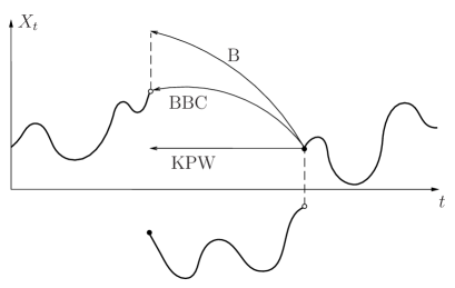
Figure 1: The construction of three related processes from $X$, the stable process: ‘B’ is the stable process conditioned to stay positive [Ber-split]; ‘BBC’ is the censored stable process [BBC-cens]; and ‘KPW’ is the process $Y$ in this work.

We now consider the pssMp $Y$ more closely for different values of $\alpha\in(0,2)$. Taking account of BertoinLP and the discussion immediately above it we know that for $\alpha\in(0,1]$, points are polar for $X$. That is, $T_{0}=\infty$ a.s., and so in this case $Y=\check{Y}$. Meanwhile, for $\alpha\in(1,2)$, every point is recurrent, so $T_{0}<\infty$ a.s.. However, the process $X$ makes infinitely many jumps across zero before hitting it. Therefore, in this case $Y$ approaches zero continuously. In fact, it can be shown that, in this case, $\check{Y}$ is the recurrent extension of $Y$ in the spirit of [RiveroRE1] and [Fitz].

Now, let $\xi=(\xi_{s})_{s\geq 0}$ be the Lamperti transform of $Y$. That is,

$$\xi_{s}=\log Y_{T(s)},\qquad s\geq 0,$$ (6)

where $T$ is a time-change. As in Section 2, we will write $\mathbb{P}_{y}$ for the law of $\xi$ started at $y\in\mathbb{R}$; note that $\mathbb{P}_{y}$ corresponds to $\mathrm{P}_{\exp(y)}$. The space transformation (6), together with the above comments and, for instance, the remark on p. 34 of [BertoinLP], allows us to make the following distinction based on the value of $\alpha$.

1. If $\alpha\in(0,1)$, $T_{0}=\infty$ and $X$ (and hence $Y$) is transient a.s.. Therefore, $\xi$ is unkilled and drifts to $+\infty$.

2. If $\alpha=1$, $T_{0}=\infty$ and every neighbourhood of zero is an a.s. recurrent set for $X$, and hence also for $Y$. Therefore, $\xi$ is unkilled and oscillates.

3. If $\alpha\in(1,2)$, $T_{0}<\infty$ and $Y$ hits zero continuously. Therefore, $\xi$ is unkilled and drifts to $-\infty$.

Furthermore, we have the following result.

Proposition 3.4.

The Lévy process $\xi$ is the sum of two independent Lévy processes $\xi^{\mathrm{L}}$ and $\xi^{\mathrm{C}}$, which are characterised as follows:

1. The Lévy process $\xi^{\mathrm{L}}$ has characteristic exponent

   $$\Psi^{*}(\theta)-c_{-}/\alpha,\qquad\theta\in\mathbb{R},$$

   where $\Psi^{*}$ is the characteristic exponent of the process $\xi^{*}$ defined in Section 2. That is, $\xi^{\mathrm{L}}$ is formed by removing the independent killing from $\xi^{*}$.

2. The process $\xi^{\mathrm{C}}$ is a compound Poisson process whose jumps occur at rate $c_{-}/\alpha$.

Before beginning the proof, let us make some preparatory remarks. Let

$$\tau=\inf\{t>0:X_{t}<0\}\quad\text{and}\quad\sigma=\inf\{t>\tau:X_{t}>0\}$$

be hitting and return times of $(-\infty,0)$ and $(0,\infty)$ for $X$. Note that, due to the time-change $\gamma$, $Y_{\tau}=X_{\sigma}$, while $Y_{\tau-}=X_{\tau-}$. We require the following lemma.

Lemma 3.5.

The joint law of $(X_{\tau},X_{\tau\!-},X_{\sigma})$ under $\mathrm{P}_{x}$ is equal to that of $(xX_{\tau},xX_{\tau\!-},xX_{\sigma})$ under $\mathrm{P}_{1}$.

Proof.

This can be shown in a straightforward way using the scaling property. ∎

Proof of Proposition 3.4.

First we note that, applying the strong Markov property to the $\left(\mathscr{G}_{t}\right)_{t\geq 0}$-stopping time $\tau$, it is sufficient to study the process $(Y_{t})_{t\leq\tau}$.

It is clear that the path section $(Y_{t})_{t<\tau}$ agrees with $(X_{t})_{t<\tau_{0}^{-}}$; however, rather than being killed at time $\tau$, the process $Y$ jumps to a positive state. Recall now that the effect of the Lamperti transform on the time $\tau$ is to turn it into an exponential time of rate $c_{-}/\alpha$ which is independent of $(\xi_{s})_{s<S(\tau)}$. This immediately yields the decomposition of $\xi$ into the sum of $\xi^{\mathrm{L}}:=(\xi^{\mathrm{L}}_{s})_{s\geq 0}$ and $\xi^{\mathrm{C}}:=(\xi^{\mathrm{C}}_{s})_{s\geq 0}$, where $\xi^{\mathrm{C}}$ is a process which jumps at the times of a Poisson process with rate $c_{-}/\alpha$, but whose jumps may depend on the position of $\xi$ prior to this jump. What remains is to be shown is that the values of the jumps of $\xi^{\mathrm{C}}$ are also independent of $\xi^{\mathrm{L}}$.

By the remark at the beginning of the proof, it is sufficient to show that the first jump of $\xi^{\mathrm{C}}$ is independent of the previous path of $\xi^{\mathrm{L}}$. Now, using only the independence of the jump times of $\xi^{\mathrm{L}}$ and $\xi^{\mathrm{C}}$, we can compute rCl ΔY_τ := Y_τ - Y_τ- &= exp(ξ^L_S(τ) + ξ^C_S(τ)) - exp(ξ^L_S(τ)- + ξ^C_S(τ) -)
= exp(ξ_S(τ)-) [ exp(Δξ^C_S(τ)) - 1 ]
= X_τ​ - [ exp(Δξ^C_S(τ)) - 1 ] , where $S$ is the Lamperti time change for $Y$, and $\Delta\xi^{\mathrm{C}}_{s}=\xi^{\mathrm{C}}_{s}-\xi^{\mathrm{C}}_{s-}$. Now,

$$\exp(\Delta\xi^{\mathrm{C}}_{S(\tau)})=1+\frac{\Delta Y_{\tau}}{X_{{\tau\!-}}}=1+\frac{X_{\sigma}-X_{{\tau\!-}}}{X_{\tau\!-}}=\frac{X_{\sigma}}{X_{\tau\!-}}.$$

Hence, it is sufficient to show that $\frac{X_{\sigma}}{X_{\tau\!-}}$ is independent of $(X_{t},t<\tau)$. The proof of this is essentially the same as that of part (iii) in Theorem 4 from CPR, which we reproduce here for clarity.

First, observe that one consequence of Lemma 3.5 is that, for $g$ a Borel function and $x>0$,

$$\mathrm{E}_{x}\biggl{[}g\biggl{(}\frac{X_{\sigma}}{X_{\tau\!-}}\biggr{)}\biggr{]}=\mathrm{E}_{1}\biggl{[}g\biggl{(}\frac{X_{\sigma}}{X_{\tau\!-}}\biggr{)}\biggr{]}.$$

Now, fix $n\in\mathbb{N}$, $f$ and $g$ Borel functions and $s_{1}<s_{2}<\dotsb<s_{n}=t$. Then, using the Markov property and the above equality, rCl E_1 [ f(X_s_1, …, X_t) g( XσXτ​ - ) 1_(t ¡ τ) ]