Modeling Tiered Pricing in the Internet
Transit Market

Abstract

ISPs are increasingly selling “tiered” contracts, which offer Internet connectivity to wholesale customers in bundles, at rates based on the cost of the links that the traffic in the bundle is traversing. Although providers have already begun to implement and deploy tiered pricing contracts, little is known about how such pricing affects ISPs and their customers. While contracts that sell connectivity on finer granularities improve market efficiency, they are also more costly for ISPs to implement and more difficult for customers to understand. In this work we present two contributions: (1) we develop a novel way of mapping traffic and topology data to a demand and cost model; and (2) we fit this model on three large real-world networks: an European transit ISP, a content distribution network, and an academic research network, and run counterfactuals to evaluate the effects of different pricing strategies on both the ISP profit and the consumer surplus. We highlight three core findings. First, ISPs gain most of the profits with only three or four pricing tiers and likely have little incentive to increase granularity of pricing even further. Second, we show that consumer surplus follows closely, if not precisely, the increases in ISP profit with more pricing tiers. Finally, the common ISP practice of structuring tiered contracts according to the cost of carrying the traffic flows (e.g., offering a discount for traffic that is local) can be suboptimal and that dividing contracts based on both traffic demand and the cost of carrying it into only three or four tiers yields near-optimal profit for the ISP.

1 Introduction

The increasing commoditization of Internet transit is changing the landscape of the Internet bandwidth market. Although residential Internet Service Providers (ISPs) and content providers are connecting directly to one another more often, they must still use major Internet transit providers to reach most destinations. These Internet transit customers can often select from among dozens of possible providers [35]. As major ISPs compete with one another, the price of Internet transit continues to plummet: on average, transit prices are falling by about 30% per year [31].

As a result of such competition, ISPs are evolving their business models and selling transit to their customers in many ways to try to retain profits. In particular, many transit ISPs today are increasingly implementing pricing strategies where wholesale Internet transit is priced by volume or destination. For example, ISPs charge prices on traffic bundles based on factors, such as how far the traffic is traveling, and whether the traffic is “on net” (i.e., to that ISP’s customers) or “off net” [15]. Still, we understand very little about the efficiency of such pricing schemes. In this work, we study destination-based tiered pricing, with the goal of understanding how tiered pricing affects ISP profit and consumer surplus.

Although understanding the effects of different transit pricing structures is important, modeling them is quite difficult. The model must take as an input existing customer demand and predict how traffic (and, hence, ISP profit and consumer surplus) would change in response to pricing strategies. Such a model must capture how customers would respond to any pricing change—for any particular traffic flow—as well as the change in cost of forwarding traffic on various paths in an ISP’s network. Of course, many of these input values are difficult to come by even for network operators, but they are especially elusive for researchers; additionally, even if certain values such as costs are known, they change quickly and differ widely across ISPs.

The model we develop allows us to estimate the relative effects of tiered pricing scenarios, despite the lack of availability of precise values for many of these parameters. The general approach, which we describe in Section 3, is to start with a demand and cost model and assume both that ISPs are already profit-maximizing and that the current prices reflects both customer demand and the underlying network costs. These assumptions allow us to either fix or solve for many of the unknown parameters and run counterfactuals to evaluate the relative effects of dividing the customer demand into pricing tiers. To drive this model, we use traffic data from three real-world networks: a major international content distribution network with its own network infrastructure; an European transit ISP; and an academic research network. We map the demand and topology data from these networks to a model that reflects the service offerings that real-world ISPs use.

Using our model and the datasets, we evaluate how the tiered pricing impacts ISPs and consumers. According to economic theory prescriptions, as we increase pricing granularity, we would expect to observe two trends: 1) ISPs should increase their profit with more tiers and 2) the marginal profit increase should be diminishing with the number of tiers. As we confirm (or refute) these predictions, we also hope to find answer to these two questions:

• How many pricing tiers ISPs need to introduce to maximize their profit? ISPs today usually use 2 to 6 pricing tiers. If, for instance, we show that a greater number of tiers provides a tangible benefit, the ISPs could rethink their current pricing policies.

• How does consumer surplus change with an increasing number pricing tiers? In abstract, a more granular pricing should lead to a better resource allocation efficiency, thus increasing the consumer surplus. If, on the other hand, we find a significant drop in consumer surplus, policy makers could take the results of such modeling into account when reviewing regulations of the Internet transit market.

• What are the best ways for ISPs to structure the pricing tiers? When ISPs use limited number of pricing tiers, they have do decide which destinations to bundle together for uniform pricing. Today, ISPs, when they use tiered pricing, usually group destinations based on cost (e.g., pricing local traffic cheaper than global traffic). We will evaluate different destination bundling strategies to see if the current approach is adequate.

As we look for answer to these questions, we make the following four contributions. First, to analyze the effects of tiered pricing, we develop a model that captures demands and costs in the transit market. One of the challenges in developing such a model is applying it to real traffic data, given many unknown parameters (e.g., the cost of various resources, or how users respond to price). Hence, we devise methods for fitting empirical traffic demands to theoretical cost and demand models (Section 3). Second, we apply our model to real-world traffic matrices and network topologies to characterize the effects of tiered pricing on the ISP profit and consumer surplus. Third, we evaluate six algorithms to structure the pricing tiers (Section 4). Fourth, we perform robustness analysis of our model, to see if results hold for a range of input parameters (Section 4.3). We wrap up the work with a review of related work and conclusion (Sections 6 and 7). Before we start, however, in the next section we present the overview the examples of tiered pricing and explain why is it beneficial to ISPs.

2 Background

In this section, we describe the current state of affairs in the Internet transit market. We first taxonomize what services (bundles) ISPs are selling. We then provide intuition on why ISPs are moving towards tiered wholesale Internet transit service.

2.1 Current Transit Market Offerings

Unfortunately, there is not much public information about the wholesale Internet transit market. ISPs are reluctant to reveal specifics about their business models and pricing strategies to their competitors. Therefore, to obtain most of the information in this section, we engaged in many discussions and email exchanges with network operators. Below, we classify the types of Internet transit service we identified during these conversations. Although much of the information in this section is widely known in the network operations community, it is difficult to find a concise taxonomy of product offerings in the wholesale transit market. The taxonomy below serves as a point of reference for our discussions of tiered pricing in this paper, but it may also be useful for anyone who wishes to better understand the state of the art in pricing strategies in the wholesale transit market.

Peering business relationships (or, more formally, settlement-free peering relationships) have been extensively studied by networking researchers [19, 8, 11, 14, 13] and well-documented in the industry white papers [31]. Most peering connections are established through public Internet eXchange Points (IXP), while higher bandwidth peering often requires private peering sessions. A network engaging in a settlement free peering allows its peer to reach on-net destinations—destinations in its own network, and destinations in customer networks. For the peering to be settlement-free, most ISPs pose a set of requirements to prospective peers, such as number of interconnection points, geographic coverage, or ingress/egress traffic ratios. If an ISP cannot meet peering requirements, it is forced to buy Internet transit or paid peering [36, 7, 23].

Transit. Most ISPs offer conventional Internet transit service. Internet transit is sold at a blended rate—a single price (usually expressed in $/Mbps/month)—charged for traffic to all destinations. Historically, blended rates have been decreasing by 30% each year [31]. Blended rate is the simplest and yet the most crude way to charge for traffic. If network costs are highly variable, less costly flows in the blended-rate bundle subsidize other, more expensive flows. ISPs often innovate by offering more than one rate: We summarize three pricing models that require two or more rates: (1) paid peering, (2) backplane peering, and (3) regional pricing.

Paid peering is similar to settlement-free peering, except that one network pays to reach the other. A major ISP might separately sell off-net routes (wholesale transit) at one rate and on-net routes (to reach destinations inside its own network) at another (usually lower) rate. For example, national ISPs in Eastern Europe, Australia, and in other regions may sell local connectivity at a discount to increase demand for local traffic, which is is significantly cheaper than transit to outside global destinations [1]. The on-net routes are also offered at a discount by some major transit ISPs to large content providers, because such transit ISPs can recoup part of the costs from their customers, who congest paid upstream links to transit ISPs by downloading the content. Some instances of paid peering have spawned significant controversy: most recently, Comcast—primarily a network serving end-users—was accused of a network neutrality violation when it forced one tier-1 provider to pay to reach Comcast’s customers [24].

Backplane peering occurs when an ISP, in addition to selling global transit through its own backbone, charges a discount rate for the traffic it can offload to its peers at the same Internet exchange. Smaller ISPs buy such a service because they might not meet all the settlement-free peering requirements to peer directly with the ISPs in the exchange. Although many large ISPs discourage this practice, some ISPs deviate by offering backplane peering to retain customers or to maintain traffic ratios with their peers. As with paid peering, the ISP selling backplane peering has to account and charge for at least two traffic flows: one to peers and another to its backbone.

Regional pricing occurs when transit service providers offer different rates to reach different geographic regions. The regions can be defined at different levels of granularity, such as PoP, metro area, regional area, nation, or continent. In some instances, the transit ISP offers access to all regions with different prices; in other instances, the downstream network purchases access only to a specific geographic region (e.g., access only to South America or Australia). In practice, due to the overhead of provisioning and maintaining many sessions to the same customer, ISPs rarely use more than one or two extra price levels for different regions.

We speculate that the bundling strategies described above arose primarily from operational and cost considerations. For example, it is relatively easy for a transit ISP to tag which routes are coming from customers and which routes are coming from peers and then in turn sell them separately to its customers. Similarly, it is relatively easy to sell local (i.e., less costly) routes separately. We show that these naïve bundling strategies might not be as effective as bundling strategies that account for both cost and demand.

2.2 The Trend Towards Tiered Pricing

Conventional blended rate pricing is simple to implement, but it may be inefficient. ISPs can lose profit as a result of blended-rate pricing, and customers can lose surplus. This is an example of market failure, where goods are not being efficiently allocated between participants of the market. Another outcome of blended-rate pricing is the increase in direct peering to circumvent “one-size-fits-all” transit. Both phenomena provide incentives for ISPs to improve their business models to retain revenue. We now explain each of these outcomes.

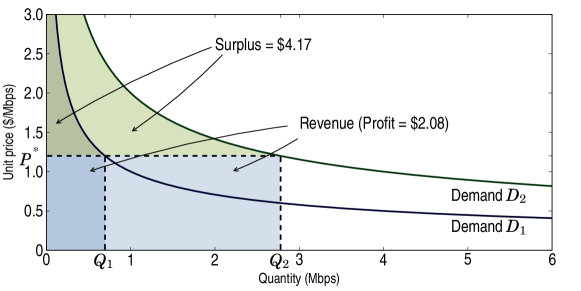
(a) Blended-rate pricing. ISP charges a single blended rate $P_{0}$.

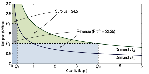
(b) Tiered pricing. ISP charges rates $P_{1}$ and $P_{2}$ for flows.

Figure 1: Market efficiency loss due to coarse bundling.

2.2.1 Profit and surplus loss

Selling transit at a blended rate could reduce profit for transit ISPs and surplus for customers. We define an ISP’s profit as its revenue minus its costs, and customer surplus as customer utility minus the amount it pays to the ISP. Unrealized profit and surplus can occur when ISPs charge a single rate while incurring different costs when delivering traffic to destinations.

Figure 1 illustrates how tiered pricing can increase both the profit for an ISP and the surplus for a customer. The downward-sloping curves represent consumer demand to two destinations. Since the demand slope $D_{2}$ is higher than demand slope $D_{1}$, the customer has higher demand for the second destination in the ISP’s network. Assume that the ISP cost of serving demand $D_{1}$ is $1, while the cost of serving demand $D_{2}$ is $0.5. Modeling demand with constant elasticity (Section 3), the profit maximizing price can be shown to be $P_{0}=\$1.2/Mbps$. If, however, the ISP is able to offer two bundles, then the profit maximizing prices for such bundles would be $P_{1}=\$2.7$ and $P_{2}=\$1$. Figure 1(b) shows that this price setup not only increases ISP profit but also increases consumer surplus and thus social welfare.

The market achieves higher efficiency because customers adjust their consumption levels of the ISP network according to their demand and to the prices that the ISP exposes, which directly depend on its costs. Without the ISP’s indirect exposure of its costs, the customer consumes less of the cheaper capacity and more of the expensive capacity than it would otherwise. In Section 3, we formalize the market that we have used in this example and propose more complex demand and cost models.

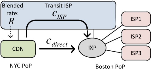
Figure 2: The customer procures a direct link if the cost for such a link is lower than the blended rate $c_{direct}<R$.

2.2.2 Increase in direct peering

Charging for traffic at a blended rate also provides incentives for client networks to connect directly to georgraphically close Internet Exchange Points (IXPs). For instance, if a transit ISP charges only blended rate, client network might find geographically close IXPs cheaper to reach by leasing or purchasing private links. While direct peering is generally perceived as a positive phenomenon, for transit ISPs it means less revenue. Direct peering efforts can also diminish economies of scale: instead of using shared ISP infrastructure, customers provision their own connectivity to IXPs.

Figure 2 illustrates an interaction between an upstream ISP and a CDN client (e.g., Google, Microsoft) with its own backbone, which extends to the NYC PoP. The CDN might, or might not, have a content cache at the Boston IXP, but since it does not have its own backbone presence at the IXP, the CDN must pay the upstream ISP to reach it. The ISP offers a blended rate $R$ at the the NYC PoP for all the traffic, including the traffic to the Boston IXP. The blended rate $R$ is set to compensate the upstream provider for the overall traffic mix and, therefore, is higher than the amortized cost of most of the cheaper (more localized) flows that ISP is serving (i.e., the flows between the NYC and Boston PoPs). The CDN eventually will procure a direct link to the Boston IXP, if it finds that it can procure such a direct link at an amortized cost $c_{direct}<R$. Assuming the ISP’s profit margin is $M$ and flow accounting overhead is $A$ (discussed in Section 5.2), such a direct link presents a market failure if $c_{direct}>(M+1)c_{ISP}+A$, because the customer deploys additional capacity at a higher cost than the ISP could have charged in a tiered market.

Some operators we interviewed confirm that they periodically re-evaluate transit bills and expand their backbone coverage if they find that having own presence in an IXP pays off. In today’s transit market, many customers increasingly opt for direct peering [21]; transit service providers are absorbing losses as a result of competitive pressure [31]. Naturally, this pressure increases the incentive for ISPs to adopt a tiered pricing model for local traffic. The central question, then, is how they should go about structuring these tiers. The rest of the paper focuses on this question.

3 Modeling Profits, Costs, and
Demands

We develop demand and cost models that capture ISP profit under various pricing strategies. Since no model can perfectly capture demand in the Internet transit market, we perform our evaluation with two commonly used demand models. Because cost is also difficult to model, we devise four network cost models. We first define ISP profit and then describe demand and cost models.

3.1 ISP Profit

We consider a transit market with multiple ISPs and customers. Each ISP is rational and maximizes its profit, which we express as the difference between its revenue and costs:

$$\Pi(\vec{P})=\textstyle\sum_{i=1}^{n}\left(p_{i}Q_{i}(\vec{P})-c_{i}Q_{i}(\vec{P})\right)$$ (1)

where $n$ is the number of flows ISP is serving, $p_{i}\in\vec{P}$ is the price an ISP sets to deliver flow $i$, $c_{i}$ is the unit cost for $i$, and $Q_{i}(\vec{P})=q_{i}$ is the demand for $i$ given a vector of prices $\vec{P}=(p_{1},p_{2},\ldots,p_{n})$. An ISP chooses the price vector $\vec{P}$ that maximizes its profit (in case when ISP is using only single pricing tier, the prices are effectively set to $p_{1}=p_{2}\cdots=p_{n}$).

Given knowledge of both the traffic demand of customers and the costs associated with delivering each flow, we can compute ISP profit. Unfortunately, it is difficult to validate any particular demand function or cost model; even if validation were possible, it is likely that cost structures and customer demand could change or evolve over time. Accordingly, we evaluate ISP profit for various tiered pricing approaches under a variety of demand functions and cost models. Section 3.2 describes the demand functions that we explore, and Section 3.3 describes the cost models that we consider.

3.2 Customer Demand

To compute ISP profit for each pricing scenario, we must understand how customers adjust their traffic demand in response to price changes. We consider two families of demand functions: constant elasticity and logit.

Constant elasticity demand. The constant elasticity demand (CED) is derived from the well-known alpha-fair utility model [28], which is often used to model user utility on the Internet. The alpha-fair utility takes the form of a concave increasing utility function, which emulates a decreasing marginal benefit to additional bandwidth for a user. In this model flow demands are separable (i.e., changes in demand or prices for one flow have no effect on demand and prices of other flows). The CED model is most appropriate for scenarios when consumers have no alternatives (e.g., when the content that a customer is trying to reach is not replicated, or the customer needs to communicate with a specific endpoint on the network).

Logit demand. To capture the fact that customers might sometimes have a choice between flows (e.g., sending traffic to alternative destination if the current one becomes too expensive), we also perform our analysis using the logit model, where demands are not separable: the price and demand for any flow depend on prices and demands for the other flows. The logit model is frequently used for this purpose in econometric demand estimation [26]. In the logit model, each consumer nominally prefers the flows that offers the highest utility. This matches well with scenarios when consumers have several alternatives (e.g., when requested content is replicated in multiple places).

3.2.1 Constant elasticity demand

Figure 3: Feasible CED demand functions for $v=1$.

The CED demand function is defined as follows:

$$Q_{i}(p_{i})=\left(\frac{v_{i}}{p_{i}}\right)^{\alpha}$$ (2)

where $p_{i}$ is the unit price (e.g., $/Mbit/s), $\alpha\in(1,\infty)$ is the price sensitivity, and $v_{i}>0$ is the valuation coefficient of flow $i$. The demand function can be interpreted to represent either inherent consumer demand or residual consumer demand, which reflects not only the inherent demand but also the availability of substitutes.

Figure 3 presents example CED demand functions for $v=1$ and two values of $\alpha$, $3.3$ and $1.4$. Higher values of $\alpha$ indicate high elasticity (users reduce use even due to small changes in price). For example, the demand with elasticity $\alpha=3.3$ might represent the traffic from residential ISPs, who are more sensitive to wholesale Internet prices and who respond to price changes in a more dramatic way. Similarly, the demand with elasticity $\alpha=1.4$ might represent the traffic from enterprise customers, who are less sensitive to the Internet transit price changes. Although our model does not capture full dynamic interaction between competing ISPs (e.g., price wars), modeling demand as residual allows us to account for the existing competitive environment and switching costs. As discussed above, high elasticity can also indicate that competitors are offering more affordable substitutes, and that switching costs for customers are low. In our evaluation, we use a range of price sensitivity values to measure how ISP profit changes for different values of the elasticity of user demand. The gray area in Figure 3 shows that we can cover all feasible demand functions simply by varying $\alpha$.

CED profit. Using the expressions for ISP profit (Equation 1) and demand (Equation 2), and assuming separability of demand of different flows, the ISP profit is:

$$\Pi(\vec{P})=\textstyle\sum_{i=1}^{n}\left(\frac{v_{i}}{p_{i}}\right)^{\alpha}\left(p_{i}-c_{i}\right).$$ (3)

CED profit-maximizing price. By differentiating the profit, we find the profit-maximizing price for each flow $i$:

$$p_{i}^{*}=\textstyle\frac{\alpha c_{i}}{\alpha-1}.$$ (4)

CED consumer surplus. Consumer surplus is the difference between consumer utility and the price paid. Price at the equilibrium is equal to the marginal utility, and thus we can find utility by integrating price as a function of demand ($p_{i}=v_{i}/q_{i}^{1/\alpha}$, Equation 2) in terms of $q_{i}$. Substituting in the resulting equation quantity with price and substracting the price paid, we get consumer surplus expression as function of price:

$$CS(\vec{P})=\textstyle\sum_{i=1}^{n}\left(\frac{\alpha v_{i}^{\alpha}p_{i}^{1-\alpha}}{\alpha-1}-p_{i}\right)$$ (5)

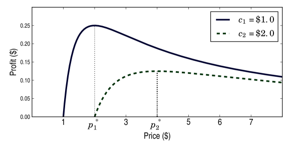
Figure 4: Profit for two flows with identical demand ($v_{1}=v_{2}=1.0$, $\alpha=2$) but different cost.

Figure 4 illustrates profit maximization for two flows that have identical demand functions but different costs. For example, the first flow costs $c_{1}=\$1.0$ per unit to deliver and mandates optimal price $p^{*}=\$2.0$ which results in $\$0.25$ profit. The second flow is more costly thus the profit maximizing price is higher. In this case, the first plot might represent profit for local traffic, while the second plot represents national traffic: ISPs must price national traffic higher than local-area traffic to maximize profit.

CED price for bundled flows. In our evaluation, we test various pricing strategies that bundle multiple flows under the same profit-maximizing price. To find the price for each bundle, we first map real world demands to our model to obtain the valuation $v_{i}$ and cost $c_{i}$ for each flow. Then, we differentiate the profit (Equation 3) with respect to the price of each bundle. For example, when we have a single bundle for all flows, we obtain the following profit-maximizing price:

$$P^{*}=\frac{\alpha\sum_{i=1}^{n}c_{i}v_{i}^{\alpha}}{(\alpha-1)\sum_{i=1}^{n}v_{i}^{\alpha}}$$ (6)

where $n$ is the number of flows. Section 4 details this approach.

3.2.2 Logit demand

The logit demand model assumes that each consumer faces a discrete choice among a set of available goods or services. In the context of data transit, the choice is between different destinations or flows. Following Besanko et al. [5], a consumer $j$ using flow $i$ will obtain the surplus:

$$u_{ij}=\alpha(v_{i}-p_{i})+\epsilon_{ij}$$

where $\alpha\in(0,\infty)$ is the elasticity parameter, $v_{i}$ is the “average” consumer’s maximum willingness to pay for flow $i$, $p_{i}$ is a price of using $i$, and $\epsilon_{ij}$ represents consumer $j$’s idiosyncratic preference for $i$ (where $\epsilon_{ij}$ follows a Gumbel distribution.) The elasticity parameter in logit demand model serves similar function to elasticity parameter in constant elasticity demand model: high $\alpha$ values represnt high elasticity (or abundance of competition), while low $\alpha$ values represent lower elasticity. The logit model defines the probability that any given consumer will use flow $i$ as a function of the price vector of all flows:

$$\textstyle s_{i}(\vec{P})=\frac{e^{\alpha(v_{i}-p_{i})}}{\sum_{j=1}^{n}e^{\alpha(v_{j}-p_{j})}+1}$$ (7)

where $\sum_{i=0}^{n}s_{i}(\vec{P})=1$. The demand for flow $i$ equals the product of $s_{i}(\vec{P})$ and the total number of consumers ($K$):

$$\textstyle Q_{i}(\vec{P})=Ks_{i}(\vec{P}).$$ (8)

Here, $s_{i}$ is also called the market share of flow $i$. The model also accounts for the possibility that some customers elect not to send traffic to any destination. The market share for traffic not sent is:

$$\textstyle s_{0}(\vec{P})=\frac{1}{\sum_{j=1}^{n}e^{\alpha(v_{j}-p_{j})}+1}.$$ (9)

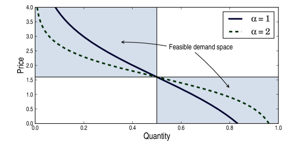
Figure 5: Logit demand function.

Figure 5 shows examples of logit demand functions. We assume a setting with two flows, with two values for the valuation $v_{i}$, $1.6$ and $1$. We fix the price for the first flow to $1$, and we vary the price for the second flow between $0$ and $4$. The figure shows demand curves for the second flow, for two values of $\alpha$. Similar to the constant elasticity demand model, lower values of $\alpha$ indicate low elasticity of demand, where users need bigger price variations to modify their usage.

Logit profit. Using the expressions for ISP profit (Equation 1) and logit demand (Equation 8), the ISP profit is:

$$\Pi(\vec{P})=\textstyle K\sum_{i=1}^{n}s_{i}(\vec{P})(p_{i}-c_{i}).$$ (10)

Logit profit-maximizing prices. To find the profit maximizing price for flow $i$, we find the first-order conditions for Equation 10:

$$p_{i}^{*}=c_{i}+\frac{1}{\alpha s_{0}}.$$ (11)

Due to the presence of $s_{0}$, $p_{i}^{*}$ recursively depends on itself and on profit-maximizing prices of other flows. To obtain maximum profit, we develop an iterative heuristic based on gradient descent that starts from a fixed set of prices ($p_{i}=P_{0},\forall i$) and greedily updates them towards the optimum.

Logit consumer surplus. After ISP sets profit-maximizing prices $\vec{P}$, we can compute consumer surplus. We find consumer surplus expression by taking the expectation of the sum of all the consumer utilities:

$$\textstyle CS(\vec{P})=K\textstyle\frac{\gamma+\ln(\textstyle\sum_{i=1}^{n}e^{\alpha(v_{i}-p_{i})}+1)}{\alpha}$$ (12)

where $\gamma$ is Euler’s constant [2].

Valuation and cost of bundled flows. To test pricing strategies, we first map real traffic demands to the model to find the valuation $v_{i}$ and cost $c_{i}$ for each flow $i$. We then bundle the flows as described in Section 4.2.1. Knowing that $\sum_{i}s_{i}=1$ and applying Equation 7 allows us to compute valuations for any bundle of flows as:

$$v_{bundle}=\frac{\ln\left(\sum_{i=1}^{n}e^{\alpha v_{i}}\right)}{\alpha}$$ (13)

where $v_{i}$ are valuations of the flows in the bundle. Similarly we can find the average unit cost of combined flows in each bundle:

$$c_{bundle}=\frac{\sum_{i=1}^{n}c_{i}e^{\alpha v_{i}}}{\sum_{i=1}^{n}e^{\alpha v_{i}}}.$$ (14)

3.3 ISP Cost

Modeling cost is difficult: ISPs typically do not publish the details of operational costs; even if they did, many of these figures change rapidly and are specific to the ISP, the region, and other factors. To account for these uncertainties, we evaluate our results in the context of several cost models. We also make the following assumptions. First, we assume the more traffic the ISP carries, the higher cost it incurs. Although on a small scale the bandwidth cost is a step function (the capacity is added at discrete increments), on a larger scale we model cost as a linear function of bandwidth. Second, we assume that ISP transit cost changes with distance. Both assumptions are motivated by practice: looking only at specific instances of connectivity, the cost is a step function of distance (e.g., equipment manufacturers sell several classes of optical transceivers, where each more powerful transceiver able to reach longer distances costs progressively more than less powerful transceivers [10]). Over a large set of links, we can model cost as a smooth function of distance.

The cost models below offer only relative flow-cost valuations (e.g., flow A is twice as costly as flow B); they do not operate on absolute costs. These relative costs must be reconciled with the blended prices used to derive customer valuations. We describe methods for reconciling these values in Section 4.1. Each cost model has a generic tuning parameter, denoted as $\theta$, which we use in the evaluation.

Linear function of distance. The most straightforward way to model ISP’s costs as a function of distance is to assume cost increases linearly with distance. Although, in some cases, this model does not hold (e.g., crossing a mountain range is more expensive than crossing a region with flat terrain), we often observe that ISPs charge linearly in the distance of communication [9, 6]. As we model cost as linear function of distance, we set cost $c_{i}=\gamma d_{i}+\beta$, where $\gamma$ is a scaling coefficient that translates from relative to real costs, $\beta$ is a base cost (i.e., the fixed cost that the ISP incurs for communicating over any distance), and $d_{i}$ is the geographical distance between the source and destination served by an ISP. We describe how we determine $\gamma$ in Section 4.1. We model the base cost $\beta$ as a fraction of the maximum cost without the base component. More formally: $\beta=\theta\max_{j\in 1\cdots n}\gamma d_{j}$, where $\theta$ in this cost model is a relative base cost fraction, and $n$ is number of flows with different cost. For example, given distances 1, 10, and 100 miles, $\gamma=\$1/mile$, and $\theta=0.1$, the resulting base cost $\beta$ is $10, and thus flow costs are $11, $20, and $110. In the evaluation, we vary $\theta$ to observe the effects of different base costs. For example, low $\theta$ values (low base cost) here represent a case where link distance is the largest contributor to the total cost.

Concave function of distance. We are also aware of ISPs that price transit as a concave function of distance, which suggests that costs likely follow the same pattern. For this scenario we model the ISP’s cost as $c_{i}=\gamma(a\log_{b}d_{i}+c)+\beta$. By fitting real pricing data that follows concave pricing patterns [17, 32], we find $a\approx 0.5$, $b\approx 6$, and $c\approx 1$ for normalized prices and distance. As in the case of linear cost, we set the base offset cost $\beta=\theta\max_{j\in 1\cdots n}\gamma(a\log_{b}d_{i}+c)$. We use $\theta$ in the evaluation to change link distance contribution to the total cost.

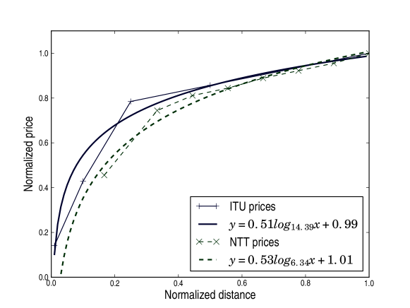
Figure 6: Using price data from ITU [17] and NTT [32] to fit concave distance to cost mapping curve.

Figure 6 shows a concave curve fitting to two price data sets, resulting in $a\approx 0.5$, $b\approx 6$, and $c\approx 1$ for normalized prices and distance. As in the case of linear cost, we set the base offset cost $\beta=\theta\max_{j\in 1\cdots n}\gamma(a\log_{b}d_{i}+c)$. We use $\theta$ in the evaluation to change link distance contribution to the total cost.

Function of destination region. Both private communication with network operators and publicly available data suggest that ISPs can also charge for traffic at rates depending on the region where traffic is destined [12, 34, 39]. For example, an ISP might have less expensive capacity in the metropolitan area than in the region, less expensive capacity in the region than in the nation, and less expensive capacity in the nation than across continental boundaries. We divide flows into three categories: metropolitan, national, and international. We map the flows into these categories by using data from the GeoIP [25] database: flows that originate and terminate in the same city are classified as metro, and flows that start and end in the same country are classified as national; all other flows are classified as international. For EU ISP we only have distances between traffic entry and exit points, thus we classify flows traveling less than 10 miles as metro, flows that travel less than 100 miles as national. We set the costs as follows: $c_{metro}=\gamma$, $c_{nation}=\gamma 2^{\theta}$, and $c_{int}=\gamma 3^{\theta}$. This form allows us to test scenarios when there is no cost difference between regions ($\theta=0$), the cost differences are linear ($\theta=1$), and costs are different by magnitudes ($\theta>1$).

Function of destination type. ISPs often offer discounts for the traffic destined to their customers (“on net” traffic), while charging higher rates for traffic destined for their peers (“off net” traffic). These offerings are motivated by the fact that ISPs do recover some of their transport cost for the traffic sent to other customers. In our evaluation, we model this cost difference by setting the cost of the traffic to peers to be twice as costly than traffic to other customers. The logic behind such a model is that when an ISP sends the traffic between two customers, it gets paid twice by both customers, but when an ISP sends traffic between a customer and a peer it is only paid by the customer. The parameter $\theta$ indicates a fraction of traffic at each distance that is destined to clients, as opposed to traffic that is destined to peers and providers.

4 Evaluating Tiered Pricing

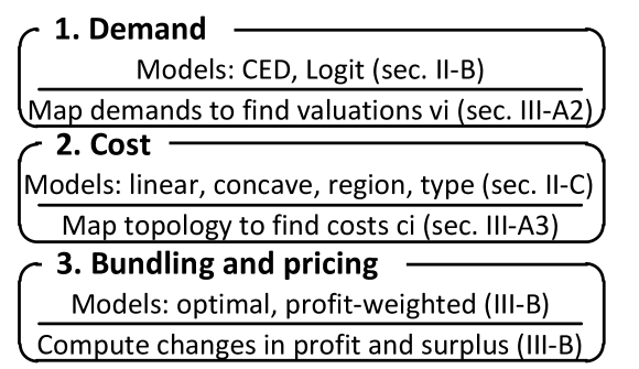
Figure 7: We evaluate the effect of tiered pricing on Internet transit by separately modeling the demand and cost of traffic. At each step we use real-world data to derive unknown parameters.

In this section, we evaluate the efficiency of destination-based tiered pricing using the model presented in Section 3 and real topology and demand data from large networks. Our goal is to understand how the consumer surplus and the profit that an ISP extracts from offering tiered-pricing depends on the number of tiers and the network topology and traffic demand. One of the major challenges we face is that we cannot know some aspects of the cost and demand models, or even which model to use. We use the ISP data to derive model parameters, such as valuation or cost, and evaluate the profit of each strategy across models and input parameters. Figure 7 presents an overview of our approach.

Our evaluation yields several important results. First, we show that an ISP needs only 3–4 bundles to capture 90–95% of the profit provided by an infinite number of bundles, if it bundles the traffic appropriately. Second, choosing a bundling strategy that considers both flow demand and cost is almost as effective as an exhaustive search for the best combination of bundles. Finally, we observe that the topology and traffic of a network influences its bundling strategies: networks with higher coefficient of variation of demand need more bundles to extract maximum profit.

4.1 Mapping Data to Models

Because we do not know the parameters that we need to compute the profit-maximizing prices we must derive them. We first describe the data then we show how to apply the demand models to the real traffic demands to compute the valuation coefficients $v_{i}$ for each flow $i$. Finally, we derive the ISP’s cost for servicing the flows by applying cost models to the observed flow distances.

Data set	Date	Distance (miles)		Traffic (Gbps)
		w-avg	CV	Aggregate	CV
EU ISP	11/12/09	54	0.70	37	1.71
CDN	12/02/09	1988	0.59	96	2.28
Internet 2	12/02/09	660	0.54	4	4.53

Table 1: Data sets used in our evaluation. The columns represent: the network, data capture date, demand-weighted average of flow distances, coefficient of variation (CV) of flow distances, aggregate traffic per second, and CV of demand of different flows.

4.1.1 Data Sources

We use demand and topology data from three networks: a European ISP serving thousands of business customers (EU ISP), one of the largest CDN providers in the world (CDN), and a major research network in United States (Internet 2). The data consists of sampled NetFlow records from core routers in each network for 24 hours. Table 1 presents more details about the data sets.

To drive our model, we must compute the traffic volume (which captures consumer demand) and the distance between the source and destination of each flow (which captures the relative cost of transit). To do so, we extract the source and destination IP, as well as the traffic level, from each NetFlow record. We obtain the demand for each flow by aggregating all records of the flow, while ensuring that we do not double-count record duplicated on different routers.

To compute distances that reflect the ISP’s cost of sending traffic, we use the following heuristics. For the EU ISP, the distance that each flow travels in the ISP’s network is the geographical distance between the flow’s entry and exit points, whose identity and location is known. For the CDN, we use the GeoIP database [25] to estimate the distance to the destination. Although this may not reflect the real distance that a packet travels (because part of the path may be covered by another ISP), we assume that it is still reflective of the cost incurred by the CDN. Finally, for Internet2 we use the router interface information to identify the links the flow has traversed. The distance each flow traverses is the sum of the links in the path, where the link length is the geographical distance between the neighboring routers.

4.1.2 Discovering valuation coefficients

The valuation coefficient $v_{i}$ indicates the valuation of flow $i$. We need the valuation coefficeint $v_{i}$ to capture how the demand for flow $i$ varies with price (Equations 2 and 8) and thus affect the ISP profit. To find $v_{i}$ for each flow, we assume that ISPs charge the same blended price $P_{0}$ for each flow and map the observed traffic demand from the data to each demand model.

CED valuation coefficient. From Equation 2 we obtain:

$$\textstyle v_{i}=P_{0}q_{i}^{1/\alpha},$$ (15)

where $q_{i}$ is observed demand on flow $i$ and $\alpha$ is the sensitivity coefficient that we vary in the evaluation.

Logit demand valuation coefficient. Dividing both left and right sides of market share expression (Equation (7) by the corresponding sides of $s_{0}$ (Equation (9)), we can find valuation of flow $i$:

$$\textstyle v_{i}=\frac{\log s_{i}-\log s_{0}}{\alpha}+P_{0},$$ (16)

where $s_{i}$ is the market share of flow $i$. We vary $s_{0}$ in the evaluation and compute the remaining market shares from observed traffic as $s_{i}=\frac{q_{i}(1-s_{0})}{\sum q_{i}}$.

4.1.3 Discovering costs

To estimate the ISP profit, we must know the cost that an ISP incurs to service each flow. However, the data provides information only about the distance each flow traverses, which reflects only the relative cost (e.g., flow A is twice as costly as flow B), rather than an absolute cost value. To normalize the cost of carrying traffic to the same units as the price for the flow, we introduce a scaling parameter $\gamma$, where $c_{i}=\gamma f(d_{i})$ and $d_{i}$ is the distance covered by $i$ (see Section 3.3). For each demand model, we compute the scaling parameter by assuming (as in computing valuation coefficients) that ISPs are rational and profit maximizing, and charge the same original price $P_{0}$ for each flow.

CED. Differentiating profit Equation (3) in terms of price and then substituting $c_{i}$ with $\gamma f(d_{i})$, we find cost normalization coefficient:

$$\gamma=\frac{P_{0}(\alpha-1)\sum_{i=1}^{n}v_{i}^{\alpha}}{\alpha\sum_{i=1}^{n}f(d_{i})v_{i}^{\alpha}}$$ (17)

Logit demand. Like in CED case, differentiating profit Equation 10 and substituting $c_{i}$ for $\gamma f(d_{i})$, we can express $\gamma$:

$$\gamma=\frac{\sum_{i=1}^{n}\left(e^{\alpha(v_{i}-P_{0})}\left(\alpha P_{0}-1-\sum_{j=1}^{n}e^{\alpha(v_{j}-P_{0})}\right)\right)}{\alpha\sum_{i=1}^{n}f(d_{i})e^{\alpha(v_{i}-P_{0})}}$$ (18)

4.2 Effects of Tiered Pricing

ISPs must judiciously choose how they bundle traffic flows into tiers. As shown in Section 2.1, today’s ISPs often offer at most two or three bundles with different prices. We define six bundling strategies that classify and group traffic flows according to their cost, demand, or potential profit to the ISP. We then evaluate them and show that, assuming the right bundling strategy is used, ISPs typically need only a few bundles to collect near-optimal profit.

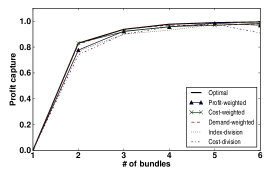
(a) European ISP.

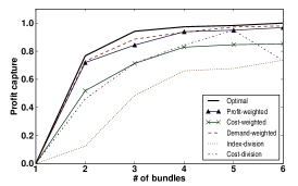
(b) Internet2.

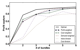
(c) International CDN.

Figure 8: Profit capture for different bundling strategies in constant elasticity demand.

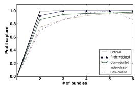
(a) European ISP.

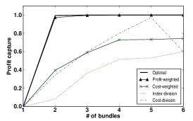
(b) Internet2.

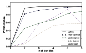
(c) International CDN.

Figure 9: Profit capture for different bundling strategies in logit demand.

4.2.1 Bundling strategies

Optimal. We exhaustively search all possible combinations of bundles to find the one that yields the most profit. This approach gives optimal results and also serves as our baseline against which we compare other strategies. Computing the optimal bundling is computationally expensive: for example, there is more than a billion ways to divide one hundred traffic flows into six pricing bundles. Presented below, all of the other bundling strategies employ heuristics to make bundling computationally tractable.

Demand-weighted. In this strategy, we use an algorithm inspired by token buckets to group traffic flows to bundles. First, we set the overall token budget as the sum of the original demand of all flows: $T=\sum_{i}q_{i}$. Then, for each bundle $j$ we assign the same token budget $t_{j}=T/B$, where $B$ is the number of bundles we want to create. We sort the flows in decreasing order of their demand and traverse them one-by-one. When traversing flow $i$, we assign it to the first bundle $j$ that either has no flows assigned to it or has a budget $t_{j}>0$. We reduce the budget of that bundle by $q_{i}$. If the resulting budget $t_{j}<0$, we set $t_{j+1}=t_{j+1}+t_{j}$. After traversing all the flows, the token budget of every bundle will be zero, and each flow will be assigned to a bundle. The algorithm leads to separate bundles for high demand flows and shared bundles for low demand flows. For example, if we need to divide four flows with demands 30, 10, 10, and 10 into two bundles, the algorithm will place the first flow in the first bundle, and the other three flows in the second bundle.

Cost-weighted. We use the same approach as in demand-weighted bundling, but we set the token budget to $T=\sum_{i}1/c_{i}$. When placing a flow in a bundle we remove a number of tokens equal to the inverse of its cost. This approach creates separate bundles for local flows and shared bundles for flows traversing longer distances. The current ISP practices of offering regional pricing and backplane peering maps closely to using just two or three bundles arranged using this cost-weighted strategy.

Profit-weighted. The bundling algorithms described above consider cost and demand separately. To account for cost and demand together, we estimate potential profit each flow could bring. We use the potential profit metric to apply the same weighting algorithm as in cost and demand-weighted bundling. In case of constant elasticity demand, we derive potential profit of each flow $i$:

$$\pi_{i}=\frac{v_{i}^{\alpha}}{\alpha}\left(\frac{\alpha c_{i}}{\alpha-1}\right)^{1-\alpha}$$ (19)

For the logit demand, substituting $p_{i}$ in Equation 11 yields:

$$\pi_{i}=Ks_{i}(p_{i}-c_{i})=\frac{Ks_{i}}{\alpha s_{0}}\propto q_{i}$$ (20)

Cost division. We find the most expensive flow and divide the cost into ranges according to that value. For example, if we want to introduce two bundles and the most expensive flow costs $10/Mbps/month to reach, we assign flows that cost $0–$4.99 to the first bundle and flows that cost $5–$10 to the second bundle.

Index division. Index-division bundling is similar to cost division bundling, except that we rank flows according to their cost and use the rank, rather than the cost, to perform the division into bundles.

4.2.2 The effects of different bundling strategies

To evaluate the bundling strategies described above, we compute the profit-maximizing prices and measure the resulting pricing outcome in terms of profit capture. Profit capture indicates what fraction of the maximum possible profit—the profit attained using an infinite number of bundles—the strategy captures. For example, if the maximum attainable profit is 30% higher than the original profit, while the profit from using two bundles is 15% higher than the original profit, the profit capture with two bundles attains 0.5 of profit capture. Formally, profit capture is $(\pi_{\mathsf{new}}-\pi_{\mathsf{original}})/(\pi_{\mathsf{max}}-\pi_{\mathsf{original}})$.

Figures 8 and 9 show the profit capture for different bundling strategies, across the three data sets, while varying the number of bundles. For the results shown here, we use both the constant elasticity and the logit demand models and the linear cost model. We set the price sensitivity $\alpha$ to $1.1$, the original, blended rate $P_{0}$ to $\$20$, the cost tuning parameter $\theta$ to $0.2$, and the original market fraction that sends no traffic $s_{0}$ to $0.2$. We explore the effect of varying these parameters in Section 4.3.

Optimal versus heuristics-based bundling. With an appropriate bundling strategy, the ISP attains maximum profit with just 3–4 bundles. As expected, the optimal flow bundling strategy captures the most profit for a given number of bundles. We observe that the EU ISP captures more profit with two bundles than other networks. We attribute this effect to the low coefficient of variation (CV) of demand to different destinations, which limits the benefits of having more pricing bundles. We also discover that, given fixed demand, a high CV of distance (cost) leads to higher absolute profits. With only minor exceptions, the profit-weighted bundling heuristic is almost as good as the the optimal bundling, followed by the cost-weighted bundling heuristic. Deeper analysis, beyond the scope of this work, could show what specific input data conditions cause the profit-weighted flow bundling heuristic to produce bundlings superior to the cost-weighted heuristic.

Logit profit capture. Maximum profit capture occurs more quickly in the logit model because (1) the total demand (including $s_{0}$ option) is constant, and (2) the model is sensitive to differences in valuation of different flows. When there is a flow with a significantly higher difference between valuation and cost ($v_{i}-c_{i}$), it absorbs most of the demand. In this model, with just two pricing tiers, local and non-local traffic are separated into distinct bundles that closely represent the backplane peering and regional pricing for local area service models.

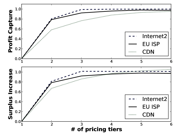
(a) Constant elasticity demand.

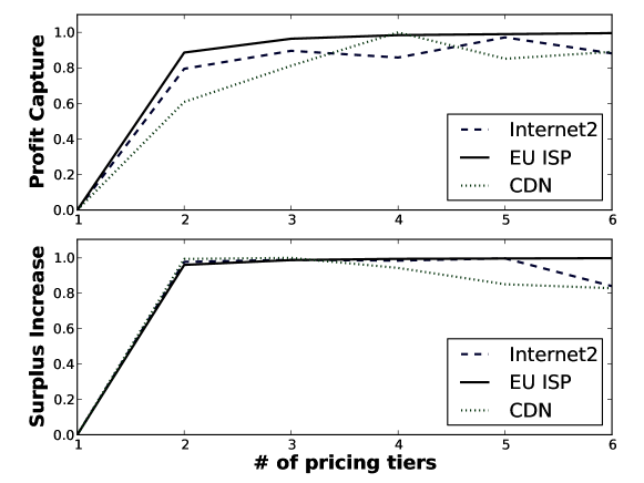
(b) Logit.

Figure 10: ISP profit and consumer surplus change as ISP employ an increasing number of pricing tiers. Concave cost model, $\theta=0.2$, $\alpha=1.1$, $s_{0}=0.2$.

4.2.3 Pricing effects on consumer surplus

Figure 10 contrasts consumer surplus change next to ISP profit gains. The consumer surplus here is normalized to the surplus gain the consumers get when ISPs maximize their profit with an infinite number of pricing tiers. As expected, the surplus gain follows closely, if not precisely, ISP profit gains.

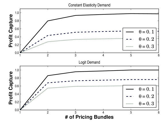
Figure 11: Profit increase in EU ISP network using linear cost model.

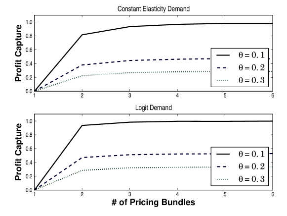
Figure 12: Profit increase in EU ISP network using concave cost model.

4.3 Sensitivity Analysis

We explore the robustness of our results to cost models and input parameter settings. As we vary an input parameter under test, other parameters remain constant. Unless otherwise noted, we use profit-weighted bundling, the EU ISP dataset, sensitivity $\alpha=1.1$, the linear cost model with base cost $\theta=0.2$, blended rate $P_{0}=\$20.0$, and, in the logit model, $s_{0}=0.2$ (the original market fraction that sends no traffic).

4.3.1 Effects of cost models

We aim to see how cost models and settings within these models qualitatively affect our results from the previous section. We show how profit changes as we increase the number of bundles for different settings of the cost model parameters ($\theta$), described in Section 3.3. We find that for different $\theta$ settings most of the attainable profit is still captured in 2-3 bundles. Unlike in other sections, in Figures 11–14, we normalize the profit of all the plots in the graphs to the highest observed profit. In other words, $\pi_{max}$ in these figures is not the maximum profit of each plot, but the maximum profit of the plot with highest profit in the figure. Normalizing by the highest observed profit allows us to show how changing the parameter $\theta$ affects the amount of profit that the ISP can capture.

Linear cost. Figure 11 shows profit increase in the EU ISP network as we vary the number of bundles for different settings of $\theta$. As expected, most of the profit is still attained with 2–3 pricing bundles. We also observe that the increase in the base cost ($\theta$) causes a decline in the maximum attainable profit. The reduction in maximum attainable profit is expected, as increasing the base cost reduces the coefficient of variation (CV) of the cost of different flows and thus reduces the opportunities for variable pricing and profit capture. We can also see, as shown in previous section, that the logit demand model attains more profit than the constant elasticity demand model with the same number of pricing bundles.

Concave cost. Figure 12 shows the profit increase as we vary the number of bundles for different settings of $\theta$ for the concave cost model. The observations and results are similar to the linear cost model, with one notable exception. The amount of profit the ISP can capture decreases more quickly in the concave cost model than in the linear cost model for the same change in the base-cost parameter $\theta$. This is due to the lower CV of cost in the concave model than in the linear cost model. In other words, applying the log function on distance (as described in Section 3.3) reduces the relative cost difference between flows traveling to local and remote destinations.

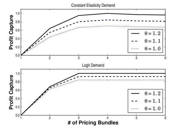
Figure 13: Profit increase in the EU ISP network using regional cost model.

Regional cost. In the regional cost model, the parameter $\theta$ is an exponent which adjusts the price difference between three different regions: local, national, and international. Figure 13 shows the profit increase in the EU ISP network as we vary number of bundles for different settings of $\theta$. Higher $\theta$ values result in a higher CV of cost in different regions which, in turn, in both demand models produces higher profit. Using constant elasticity demand we observe a small dip in profit when using five and six bundles, which recovers later with more bundles. Such dips are expected when there are only a few traffic classes. For example, if traffic had just two distinct cost classes, two judiciously selected bundles could capture most of the profit. Adding a third bundle can reduce the profit if that third bundle contains flows from both of the classes (as may happen in a suboptimal bundling).

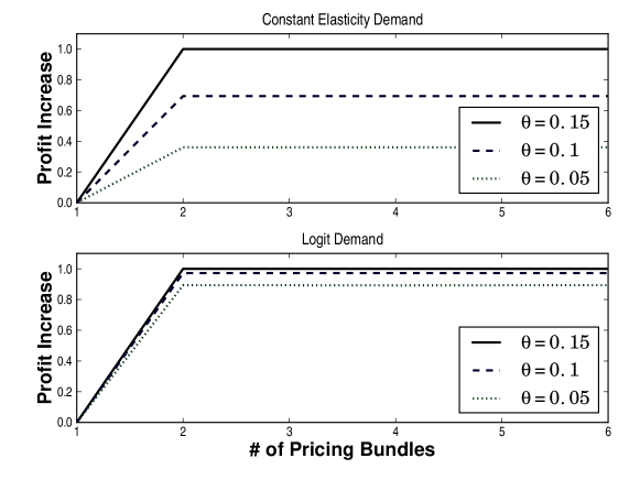
Figure 14: Profit increase in the EU ISP network using destination type cost model.

Destination type-based cost. Destination type-based cost model emulates “on-net” and “off-net” types of traffic in an ISP network. As described in Section 3.3, we assume that “on-net” traffic costs less than “off-net” traffic. We vary $\theta$, which represents a fraction of “on-net” traffic in each flow. The standard profit-weighting algorithm does not work well with the destination type-based cost model. The effect observed in the regional cost model—where five bundles produce slightly lower profit then four bundles—is more pronounced when we have just two distinct flow classes. One heuristic that works reasonably well is as follows: we update the profit-weighting heuristic to never group traffic from two different classes into the same bundle. Figure 14 shows how profit increases with an increasing number of bundles. Since there are two major classes of traffic (“on-” and “off-net”), most profit is attained with two bundles for both demand models. In this cost model, as in other cost models, the same change in CV of cost (induced by the parameter $\theta$) causes a greater change in profit capture for constant elasticity demand than for logit demand.

4.3.2 Sensitivity to parameter settings

The models we use rely on a set of parameters, such as price sensitivity ($\alpha$), price of the original bundle ($P_{0}$), and, in the logit model, the share of the market that corresponds to deciding not to purchase bandwidth ($s_{0}$). In this section, we analyze how sensitive the model is to the choice of these parameters.

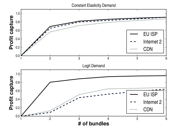
Figure 15: Minimum profit capture for a fixed number of bundles over a range of $\alpha$ between 1 and 10.

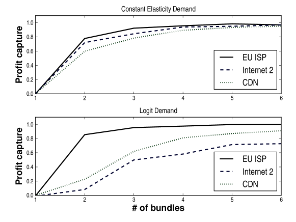
Figure 16: Minimum profit capture for a fixed number of bundles over a range of starting prices $P_{0}\in[5,30]$.

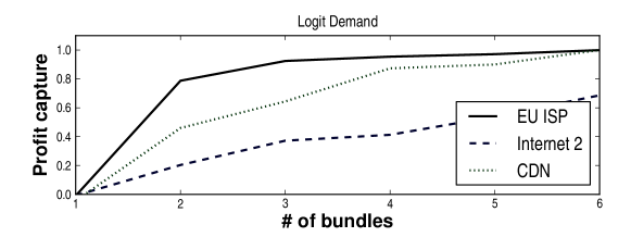
Figure 17: Maximum profit capture for a fixed number of bundles over a range of fractions of users who decide not to participate in the market $s_{0}\in(0,1)$.

Figures 15–17 show how profit capture is affected by varying price sensitivity $\alpha$, blended rate $P_{0}$, and non-buying market share $s_{0}$, respectively. Each data point in the figures is obtained by varying each parameter over a range of values. We vary $\alpha$ between 1 and 10, $P_{0}$ between 5 and 30, and $s_{0}$ between 0 and 0.9. As we vary the parameters, we select and plot the minimum observed profit capture over the whole parameter range, for the profit-weighted strategy with different numbers of bundles. In other words, these plots show the worst case relative profit capture for the ISP over a range of parameter values. The trend of these minimum profit capture points is qualitatively similar to patterns in Figures 8 and 9. For example, using the CED model and grouping flows in two bundles in the EU ISP yields around 0.8 profit capture, regardless of price sensitivity, blending rate, and market share. These results indicate that our model is robust to a wide range of parameter values.

5 Implementing Tiered Pricing

ISPs can implement the type of tiered pricing that we describe in Section 4 without any changes to their existing protocols or infrastructure, and ISPs may already be using the techniques we describe below. If that is the case, they could simply apply a profit-weighted bundling strategy to re-factor their pricing to improve their profit, possibly without even making many changes to the network configuration. We describe two tasks associated with tiered pricing: associating flows with tiers and accounting for the amount of traffic the customer sends in each tier.

5.1 Associating Flows with Tiers

Associating each flow (or destination) with a tier can be done within the context of today’s routing protocols. When the upstream ISP sends routes to its customer, it can “tag” routes it announces with a label that indicates which tier the route should be associated with; ISPs can use BGP extended communities to perform this tagging. Because the communities propagate with the route, the customer can establish routing policies on every router within its own network based on these tags.

Suppose that a large transit service provider has routers in different geographic regions. Routers at an exchange point in, say, New York, might advertise routes that it learned in Europe with a special tag indicating that the path the route takes is trans-Atlantic and, hence, bears a higher price than other, regional routes. The customer can then use the tag to make routing decisions. For example, if a route is tagged as an expensive long-distance route, the customer might choose to use its own backbone to get closer to destination instead of performing the default “hot-potato” routing (i.e., offloading the traffic to a transit network as quickly as possible). A large customer might also use this pricing information to better plan its own network growth.

5.2 Accounting

Implementing tiered pricing requires accounting for traffic either on a per-link or per-flow basis.

Link-Based Accounting. As shown in Figure 18(a), an edge router can establish two or more physical or virtual links to the customer, with a Border Gateway Protocol (BGP) [37] session for each physical or virtual link. In this setup, each pricing tier would have a separate link. Each link carries the traffic only to the set of destinations advertised over that session (e.g., on-net traffic, backplane peering traffic). Because each link has a separate routing session and only exchanges routes associated with that pricing tier, the customer and provider can ensure that traffic for each tier flows over the appropriate link: The customer knows exactly which traffic falls into which pricing tier based on the session onto which it sends traffic. Billing may also be simpler and easier to understand, since, in this mode, a provider can simply bill each link at a different rate. Unfortunately, the overhead of this accounting method grows significantly with the number of pricing levels ISP intends to support.

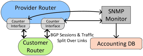
(a) SNMP-Based Accounting.

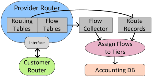
(b) Flow-Based Accounting.

Figure 18: Implementing accounting for tiered pricing.

Flow-Based Accounting. In flow-based accounting, as in traditional peering and transit, an upstream ISP and a customer establish a link with a single routing session. As shown in Figure 18(b), the accounting system collects both flow statistics (e.g., using NetFlow [30]) and routing information to determine resource usage. For the purposes of accounting, bundling effectively occurs after the fact: flows can be mapped to distances using the routing table information and priced accordingly, exactly as we did in our evaluation in Section 4. Assuming flow and routing information collection infrastructure in place, flow-based accounting may be easier to manage, and it is easier to bundle flows into different bins according to various bundling strategies (e.g., profit-weighted bundling) post facto.

6 Related Work

Developing and analyzing pricing models for the Internet is well-researched in both networking and economics. Two aspects are most relevant for our work: the unbundling of connectivity and the dimensions along which to unbundle it. Although similar studies of pricing exist, none evaluated in the context of real network demand and topology data.

The unbundling of connectivity services refers to the setting of different prices for such services along various usage dimensions such as volume, time, destination, or application type. Seminal works by Arrow and Debreu [3] and McKenzie [27] show that markets where commodities are sold at infinitely small granularities are more efficient. More recent studies however, demonstrate that unbundling may be inefficient in certain settings, such as when selling information goods with zero or very low marginal cost (such as access to online information) [4, 22, 29]. This is not always the case with the connectivity market, where ISPs incur different costs to deliver traffic to different destinations. In addition, many service providers already use price discrimination [33].

Kesidis et al. [20] and Shakkottai et al. [38] study the benefits of pricing connectivity based on volume usage and argue that, with price differentiation, one can use resources more efficiently. In particular, Kesidis et al. show that usage-based unbundling may be even more beneficial to access networks rather than core networks. Time is another dimension along which providers can unbundle connectivity. Jiang et al. [18] study the role of time preference in network prices and show analytically that service providers can achieve maximum revenue and social welfare if they differentiate prices across users and time. Hande et al. [16] characterize the economic loss due to ISP inability or unwillingness to price broadband access based on time of day.

7 Conclusion

As the price of Internet transit drops, transit providers are selling connectivity using “tiered” contracts based on traffic cost, volume, or destination to maintain profits. We have studied two questions: How does tiered pricing benefit the ISPs? and How does tiered pricing affect their customers? We developed a model for an Internet transit market that helps us to evaluate differing pricing strategies of the ISPs. We have applied our model to traffic demand and topology data from three large ISPs to evaluate various bundling strategies.

We find that the ISPs gain most of the profits with only three or four pricing tiers and likely have little incentive to icnrease granularity of pricing even further. We also show that consumer surplus follows closely, if not precisely, the increases in ISP profit with more pricing tiers.

References

- [1] Adam Internet. Unmetered content. http://www.adam.com.au/unmetered/unmetered.php. Retrieved: June 2011.
- [2] G. Ali. Expected utility in econometric random utility models. The Indian Journal of Statistics, 70(1), 2008.
- [3] K. J. Arrow and G. Debreu. Existence of equilibrium for competitive economy. Econometrica, 22(3):265–290, 1954.
- [4] Y. Bakos and E. Bronjolfsson. Bundling and competition on the Internet. Marketing Science, 19(1), Jan. 1998.
- [5] D. Besanko, S. Gupta, and D. Jain. Logit demand estimation under competitive pricing behavior: An equilibrium framework. Management Science, 44:1533–1547, Nov. 1998.
- [6] BNSL. Tariff for leased lines. http://www.bsnl.co.in/service/2mbps.pdf. Retrieved: June 2011.
- [7] M. A. Brown, A. Popescu, and E. Zmijewski. Peering Wars: Lessons Learned from the Cogent-Telia De-peering. In NANOG 43, June 2008.
- [8] H. Chang, S. Jamin, and W. Willinger. To peer or not to peer: Modeling the evolution of the Internet’s AS-level topology. In Proc. IEEE INFOCOM, Barcelona, Spain, Mar. 2006.
- [9] Chunghwa Telecom. Leased line pricelist. http://www.cht.com.tw/CHTFinalE/Web/Business.php?CatID=476. Retrieved: June 2011.
- [10] Cisco. SFP optics for gigabit ethernet applications. http://www.cisco.com/en/US/prod/collateral/modules/ps5455/ps6577/product_data_sheet0900aecd8033f885.html. Retrieved: June 2011.
- [11] A. Dhamdhere, P. Francois, and C. Dovrolis. A value based framework for internet peering agreements. In Proc. International Teletraffic Congress (ITC), 2010.
- [12] Etisalat ISP. Leased circuit rental charges. http://tinyurl.com/66tfvj6. Retrieved: June 2011.
- [13] N. Feamster and H. Balakrishnan. Verifying the correctness of wide-area Internet routing. Technical Report MIT-LCS-TR-948, Massachusetts Institute of Technology, May 2004.
- [14] N. Feamster, Z. M. Mao, and J. Rexford. BorderGuard: Detecting cold potatoes from peers. In Proc. Internet Measurement Conference, Taormina, Italy, Oct. 2004.
- [15] Guavus. Profitable tiered pricing. http://www.guavus.com/solutions/tiered-pricing. Retrieved: June 2011.
- [16] P. Hande, M. Chiang, R. Calderbank, and J. Zhang. Pricing under constraints in access networks: Revenue maximization and congestion management. In Proc. IEEE INFOCOM, San Diego, CA, Mar. 2010.
- [17] ITU Telecommunication Indicator Handbook. http://www.itu.int/ITU-D/ict/publications/world/material/handbook.html. Retrieved: June 2011.
- [18] L. Jiang, S. Parekh, and J. Walrand. Time-dependent network pricing and bandwidth trading. In Proc. IEEE BoD, 2008.
- [19] R. Johari and J. Tsitsiklis. Routing and Peering in a Competitive Internet. Technical Report LIDS Publication 2570, Massachusetts Institute of Technology, 2003. http://www.stanford.edu/~rjohari/pubs/netgamepaper.pdf.
- [20] G. Kesidis, A. Das, and G. D. Veciana. On flat-rate and usage-based pricing for tiered commodity Internet services. In Proc. CISS, 2008.
- [21] C. Labovitz, S. Iekel-Johnson, D. McPherson, J. Oberheide, and F. Jahanian. Internet inter-domain traffic. In Proc. ACM SIGCOMM, New Delhi, India, Aug. 2010.
- [22] J.-J. Laffont, S. Marcus, P. Rey, and J. Tirole. Internet interconnection and the off-net-cost principle. The Rand Journal of Economics, 34(2), 2003.
- [23] M. Leber. IPv6 Internet broken, cogent/telia/hurricane not peering. http://www.merit.edu/mail.archives/nanog/msg01006.html, Oct. 2009.
- [24] Level 3 Communications. Level 3 statement concerning Comcast’s actions. http://www.level3.com/index.cfm?pageID=491&PR=962. Retrieved: June 2011.
- [25] MaxMind GeoIP Country. http://www.maxmind.com/app/geolitecountry. Retrieved: June 2011.
- [26] D. McFadden. Conditional logit analysis of qualitative choice behavior. Frontiers Of Econometrics, 1974.
- [27] L. W. McKenzie. On the existence of general equilibrium for a competitive economy. Econometrica, 1959.
- [28] J. Mo and J. Walrand. Fair end-to-end window-based congestion control. IEEE/ACM Trans. Netw., 8(5):556–567, 2000.
- [29] P. Nabipay, A. M. Odlyzko, and Z.-L. Zhang. Flat versus metered rates, bundling, and “bandwidth hogs”. In 6th Workshop on the Economics of Networks, Systems, and Computation, San Jose, CA, June 2011.
- [30] Cisco NetFlow. http://www.cisco.com/en/US/products/ps6601/products_ios_protocol_group_home.html. Retrieved: June 2011.
- [31] W. Norton. DrPeering.net. http://drpeering.net.
- [32] NTT East. Leased circuit price list. http://www.ntt-east.co.jp/senyo_e/charge/digital.html. URL retrieved January 2011.
- [33] A. M. Odlyzko. Network neutrality, search neutrality, and the never-ending conflict between efficiency and fairness in markets. Review of Network Economics, 8(1):40–60, Mar. 2009.
- [34] ORE. Wholesale leased lines price list. http://www.otewholesale.gr/Portals/0/LEASED%20LINES_Pricelist_ENG_081110.pdf. Retrieved: June 2011.
- [35] Peering Database. http://www.peeringdb.com.
- [36] A. Popescu and T. Underwood. D(3) Peered: Just the Facts Ma¿am. A Technical Review of Level (3)¿s Depeering of Cogent. In NANOG 35, Oct. 2005.
- [37] Y. Rekhter, T. Li, and S. Hares. A Border Gateway Protocol 4 (BGP-4). Internet Engineering Task Force, Jan. 2006. RFC 4271.
- [38] S. Shakkottai, R. Srikant, A. E. Ozdaglar, and D. Acemoglu. The price of simplicity. IEEE Journal on Selected Areas in Communications, 26(7):1269–1276, 2008.
- [39] Telegeography. Bandwidth pricing report. http://www.telegeography.com/product-info/pricingdb/download/bpr-2009-10.pdf. Retrieved: June 2011.