Determining low-energy constants in partially quenched Wilson chiral perturbation theory

Abstract

In the low energy effective theory describing the partially quenched extension of two light Wilson fermions, three low energy constants (LECs) appear in terms proportional to $a^{2}$ ($a$ being the lattice spacing). We propose methods to separately calculate these LECs, typically called $W_{6}^{\prime}$, $W_{7}^{\prime}$ and $W_{8}^{\prime}$. While only one linear combination of these constants enters into physical quantities, different combinations enter into the description of the spectral density and eigenvalue distributions of the lattice Dirac operator and its Hermitian counterpart. Thus it is useful to be able to determine the LECs separately. Our methods require studying certain correlation functions for either two or three pion scattering, which are accessible only in the partially quenched extension of the theory.

I Introduction and Summary

Calculations using (improved versions) of Wilson fermions Wilson (1974) have successfully approached Giusti and Luscher (2009), and even reached Durr et al. (2011), physical light quark masses. The twisted-mass extension has also been highly successful Baron et al. (2010). Nevertheless, the explicit breaking of chiral symmetry can lead to significant lattice artefacts that need to be understood and controlled. For example, studying the long-distance behavior of Wilson fermions using chiral effective theory Sharpe and Singleton (1998); Creutz (1996), one finds that, when quark masses satisfy $m\sim a^{2}\Lambda_{\rm QCD}^{3}$ ($a$ being the lattice spacing), discretization errors lead to a non-trivial phase diagram, with one scenario (the “first-order scenario”) having a minimum pion mass, $M_{\pi}^{\rm min}\sim a\Lambda_{\rm QCD}^{2}$, and the other having a region of Aoki phase in which flavor is spontaneously broken Aoki (1984). There have also been numerous studies of the properties of mesons and baryons using the chiral effective theory—usually called Wilson chiral perturbation theory (WChPT)—which provide the functional forms needed to do simultaneous chiral and continuum extrapolations.

In the unquenched theory with two light flavors (a class of theories which includes physical QCD if one treats the strange quark as heavy), the chiral Lagrangian contains only one independent term proportional to $a^{2}$. As a result, $a^{2}$ corrections enter with a single low energy constant (LEC), denoted $c_{2}$ in Ref. Sharpe and Singleton (1998). The sign of this constant determines the vacuum structure when $m\sim a^{2}\Lambda_{\rm QCD}^{3}$. If one wants to go beyond the phase structure, however, and use the chiral effective theory to determine discretization errors in the spectral density of the Hermitian Wilson-Dirac operator Sharpe (2006), or, more generally, to determine the detailed properties of low lying eigenvalues of the Wilson-Dirac operator Damgaard et al. (2010); Akemann et al. (2011), then it turns out that one must consider the partially quenched (PQ) extension of WChPT. In this extension, there are three LECs entering in terms proportional to $a^{2}$, denoted $W_{6}^{\prime}$, $W_{7}^{\prime}$ and $W_{8}^{\prime}$ [see Eq. (15) below], of which $c_{2}$ is a particular linear combination [see Eq. (16)]. The detailed properties of the spectrum and eigenvalues depend on all three LECs and not just on $c_{2}$. It is thus of interest to determine the LECs separately, and this is the topic of the present work.

Our proposal builds upon one of the methods being used to determine $c_{2}$. This is to calculate certain pion scattering lengths (i.e. the scattering amplitudes at threshold), which in the continuum are proportional to $m$, but which also have contributions proportional to $c_{2}a^{2}$ when discretization errors are included Aoki et al. (2008). Computationally, the simplest choice is to calculate the $\pi^{+}\pi^{+}\to\pi^{+}\pi^{+}$ scattering amplitude, for this involves no quark-antiquark annihilation contractions, as illustrated in Fig. 1. The scattering length can be calculated from the energy shift $\delta E=E(\pi^{+}\pi^{+})-2m_{\pi}$ using the method of Ref. Luscher (1986). (More details of this method will be given below.) Such a calculation is in fact presently being carried out Bernardoni et al. (2011).

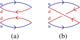
Figure 1: Quark contractions contributing to $\pi^{+}\pi^{+}$ scattering. Contractions involving the interchange of the final state pions are not shown.

Our method for calculating two of the LECs is to consider separately the quark-disconnected contraction of Fig. 1(a) and the quark-connected contraction of Fig. 1(b). This separation is simple in a numerical simulation, but it introduces a problem in the theoretical description. To pick out the separate contractions requires (for the two-flavor theory that we consider) using a PQ theory. We stress that in this application of partial quenching the valence quarks are all degenerate with the sea quarks and have the same action. This is in contrast with the most common application in which the valence and sea quark masses (and sometimes also actions) differ.

While well defined as a Euclidean field theory, the PQ theory is unphysical, and the method of Ref. Luscher (1986) for determining the scattering lengths does not apply. In particular, the individual contractions cannot be written as a sum of exponentials, as is the case for their sum. Our proposal is instead to directly fit the correlation functions calculated in the simulation to the predictions of PQWChPT. These predictions depend, at leading order (LO), on the LECs $W^{\prime}_{6}$ and $W^{\prime}_{8}$, and thus these two constants can be determined from lattice data at sufficiently small $m$ and $a^{2}$. This method of comparison was first introduced in the quenched theory Bernard and Golterman (1996). In both the quenched and PQ cases, the key point is that the effective chiral theory reproduces, at long distances, the unphysical nature of the underlying theory.

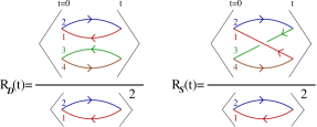
Figure 2: Ratios of partially quenched correlation functions used to extract LECs. Lines show quark propagators, with the valence flavor indicated by the label [and color]. All interpolating operators are at zero three-momentum, and are placed at the Euclidean times indicated. Expectation values are taken with two sea quarks having the same action and masses as the valence quarks.

Specifically, we suggest calculating the ratios of correlation functions shown in Fig. 2 [and defined in Eqs. (51-55) below]. This calculation must be done outside the Aoki phase, if present, as we assume that flavor is not spontaneously broken. As we show in Sec. IV, at LO in ChPT the ratios are given by

$$R_{{\cal D}}(t) = 1+\mathcal{O}(1/L^{3})+2w^{\prime}_{6}\frac{t}{4M_{\pi}^{2}L^{3}}\,,$$ (1)

$$R_{{\cal S}}(t) = \mathcal{O}(1/L^{3})+\left(w^{\prime}_{8}-\frac{M_{\pi}^{2}}{f^{2}}\right)\frac{t}{4M_{\pi}^{2}L^{3}}\,,$$ (2)

where $w^{\prime}_{6,8}$ are proportional to $W^{\prime}_{6,8}$ [see Eq. (26)], and $f\approx f_{\pi}$. Thus these two LECs can be determined from the terms linear in $t$. This requires that $t$ be large enough that contributions from excited pion states, which fall exponentially, can be neglected. It also requires that the linear terms in $t$ can be distinguished from quadratic terms which appear at higher order in ChPT and which scale as $1/L^{6}$. In practice, these conditions seem reasonable (see, e.g., Ref. Bernardoni et al. (2011)).

In a ratio of physical correlation functions, the contribution linear in $t$ is the first term in the expansion of the exponential $\exp(-\delta Et)$. In the PQ theory, by contrast, neither $R_{{\cal D}}(t)$ nor $R_{{\cal S}}(t)$ are exponentials. This is immediately clear for $R_{{\cal S}}(t)$ due to the absence of an $L$-independent constant term and will be shown explicitly for $R_{{\cal D}}(t)$ by calculating the quadratic term—see Eq. (104). Nevertheless, as long as it is possible to pick out the term linear in $t$ one can extract the LECs.

In practice, subleading terms in the chiral expansion are significant at the values of $m$ and $a^{2}$ used in present simulations. Thus we have extended the calculation of the ratios to next-to-next-to-leading order (NNLO) in the power counting appropriate to the $m\sim a^{2}$ regime (usually called the “large cut-off effects” or LCE regime). This power-counting is explained in Sec. II. It differs from the usual continuum power-counting in that one-loop effects are of NNLO, rather than next-to-leading order (NLO). The only NLO contributions are from analytic terms.

The LO results are generalized in a fairly simple way. To describe this, we first define ${\cal D}(s,t,u)$ and ${\cal S}(s,t,u)$ as the infinite volume, PQ scattering amplitudes corresponding to the contractions of Figs. 1(a) and (b) respectively [see Eqs. (9) and (10) below]. We then observe that the coefficients of $t/4M_{\pi}^{2}L^{3}$ in Eqs. (1) and (2) are simply the LO values of ${\cal D}(4M_{\pi}^{2},0,0)$ and ${\cal S}(4M_{\pi}^{2},0,0)$, the amplitudes at threshold. What we show in Sec. IV is that the coefficients of $t/(4M_{\pi}^{2}L^{3})$, when evaluated to NNLO in the chiral expansion, continue to equal the infinite-volume threshold amplitudes, also evaluated to that order. In effect, picking out the coefficient of the term linear in $t$ in the ratios is, for the threshold amplitude, like performing LSZ reduction.

The full NNLO results are given in Eqs. (104) and (105). We display here only simplified forms which show the essential features:

$$\begin{split}R_{{\cal D}}(t)&=1+{\cal O}\left(\frac{M_{\pi}^{2}}{f^{2}}\frac{1}{M_{\pi}^{3}L^{3}}\right)\\ &{}+{\cal D}(4M_{\pi}^{2},0,0)\frac{t}{4M_{\pi}^{2}L^{3}}\left[1+{\cal O}\left(\frac{M_{\pi}^{2}}{f^{2}}\frac{1}{M_{\pi}L}\right)\right]\\ &{}+{\cal O}\left(\left[\frac{M_{\pi}^{2}}{f^{2}}\frac{t}{M_{\pi}^{2}L^{3}}\right]^{2}\right)+{\cal O}(e^{-M_{\pi}L})+\mathrm{exp.suppr.}\,,\end{split}$$ (3)

$$\begin{split}R_{{\cal S}}(t)&={\cal O}\left(\frac{M_{\pi}^{2}}{f^{2}}\frac{1}{M_{\pi}^{3}L^{3}}\right)\\ &{}+{\cal S}(4M_{\pi}^{2},0,0)\frac{t}{4M_{\pi}^{2}L^{3}}\left[1+{\cal O}\left(\frac{M_{\pi}^{2}}{f^{2}}\frac{1}{M_{\pi}L}\right)\right]\\ &{}+{\cal O}\left(\left[\frac{M_{\pi}^{2}}{f^{2}}\frac{t}{M_{\pi}^{2}L^{3}}\right]^{2}\right)+{\cal O}(e^{-M_{\pi}L})+\textrm{exp. suppr.}\,,\end{split}$$ (4)

where ${\cal D}$ and ${\cal S}$ are evaluated to NNLO, and the results at threshold are given in Eqs. (106) and (107). In our “big ${\cal O}$” notation, $M_{\pi}^{2}/f^{2}$ may also stand for any of the terms proportional to $a^{2}W^{\prime}_{k}$, as these are of the same order in the LCE regime. By “exp. suppr.” we mean contributions which fall off exponentially with $t$, e.g. due to excited states.

As can be seen from Eqs. (3) and (4) there are three expansions being used. First, there is the usual chiral expansion (supplemented by powers of $a$) in the expressions for ${\cal D}$ and ${\cal S}$. Second, there is an expansion in powers of $t$, as indicated in the last lines of (3) and (4). Finally, for each power of $t$ there is a sequence of subleading terms, as is shown in the middle line of each equation.

Our calculation in Sec. IV yields the first non-trivial correction in each of these expansions, namely the chiral corrections to ${\cal D}$ and ${\cal S}$ and the contributions to the ratios proportional to $t^{2}/L^{6}$ and $t/L^{4}$. The latter two are given explicitly in (104) and (105). We stress again that, if the numerators in the ratios were physical correlation functions, then, using the results of Ref. Luscher (1986), one would find that the $t/L^{4}$ and $t^{2}/L^{6}$ terms would be proportional to the square of the threshold scattering amplitude. This is not true in the PQ theory, but one can nevertheless calculate these terms.

With the NNLO results (3) and (4) in hand, we can discuss our proposal for determining LECs in more detail. In order for the term linear in $t$ to dominate over the quadratic term, it must satisfy

$$t\ll{f^{2}L^{3}}\sim\frac{(M_{\pi}L)(fL)^{2}}{M_{\pi}}\,.$$ (5)

Since $M_{\pi}L\gg 1$ and $fL\gtrsim 1$ to avoid large finite-size effects, one sees that the constraint on $t$ is rather weak. One may also try and fit the ratios including the quadratic term, and in this regard we note that the coefficient of $t^{2}$ is given by a linear combination of $M_{\pi}^{2}/f^{2}$ and the LECs $W_{6}^{\prime}$ and $W_{8}^{\prime}$, so that no new parameters are needed.

Assuming that one can determine the coefficient of $t$, one must disentangle its dependence on $M_{\pi}^{2}$ and on $1/L$ in order to extract the LECs $W^{\prime}_{6}$ and $W^{\prime}_{8}$. Here it is helpful that the $1/L$ correction itself depends on these same two LECs. At the least, this will allow an a posteriori estimate of the size of the $1/L$ correction.

Finally, one must do a chiral extrapolation of the resulting threshold amplitudes, attempting to pick out the LO terms which give the desired LECs. From Eqs. (106) and (107), the general chiral behavior is, schematically,

$${\cal D},{\cal S} \sim a^{2}+M_{\pi}^{2}+a^{3}+aM_{\pi}^{2}+a^{4}(1+\log M_{\pi})$$ (6)

$$+a^{2}M_{\pi}^{2}(1+\log M_{\pi})+M_{\pi}^{4}(1+\log M_{\pi})\,.$$

The coefficients of the chiral logarithms are either fixed (for the continuum logarithm) or given in terms of all three $W^{\prime}_{k}$ (for the logarithms multiplying factors of $a$). The analytic terms involve many other LECs, however, both from the continuum theory and induced by discretization errors. Thus it seems very unlikely that one will be able do more than a fit to the generic form given above and extract the LO $a^{2}$ and $M_{\pi}^{2}$ terms. This would allow a determination of $W^{\prime}_{6}$ and $W^{\prime}_{8}$, but not $W^{\prime}_{7}$.

In light of this, we have devised an alternative method for determining $W_{7}^{\prime}$, in which it contributes at tree-level. This requires studying a particular three-pion correlation function. Since this will be challenging to implement in a simulation, we describe the method only briefly in an appendix.

We close this section by noting that other methods for determining $W^{\prime}_{6}$, $W^{\prime}_{7}$ and $W^{\prime}_{8}$ have recently been proposed. These use the eigenvalue distributions of the Hermitian Wilson-Dirac operator with Wilson-like fermions (which are sensitive to all three LECs) Damgaard et al. (2010); Akemann et al. (2011), the masses of pions and the scalar correlator in a mixed-action simulation with overlap valence quarks and twisted-mass sea quarks (which can determine $W^{\prime}_{6}$ and $W^{\prime}_{8}$) Cichy et al. (tion), and the mass of the quark-connected neutral pion with twisted-mass quarks (which determines $W^{\prime}_{8}$) Hansen and Sharpe (2011). We think that pinning down the LECs will not be easy, and hope the method proposed here can contribute along with these other approaches.

The remainder of this article is organized as follows. In the following section, we give a brief recapitulation of the pertinent details of PQWChPT, including the power-counting of the LCE regime. In Sec. III we present our results for the infinite-volume PQ scattering amplitudes, which we do for general momentum, and at NNLO in the LCE power counting. The description and calculation of the finite-volume correlations functions are presented in Sec. IV, which forms the core of the technical part of this paper. We include two appendices. The first contains details concerning analytic NLO and NNLO contributions to the scattering amplitudes. The second describes our proposal for determining $W^{\prime}_{7}$.

II Partially Quenched Wilson Chiral Perturbation Theory

In this section we define the required PQ scattering amplitudes and recall the essentials of WChPT for the partially quenched theory. We consider a theory with two sea quarks, and introduce four valence quarks, and their corresponding ghosts, in order to define the desired amplitudes. All quarks and ghosts are degenerate with mass $m$. With this quark content, the chiral field

$$\Sigma=\exp\left(\sqrt{2}i\pi/f\right)$$ (7)

lies in the graded group $SU(6|4)$. We work in the LCE regime where $m\sim a^{2}$, so the Lagrangian is broken into leading and subleading parts as follows Aoki et al. (2008):

$$\begin{split}{\mathrm{LO}}&:\ p^{2},m,a^{2}\\ {\mathrm{NLO}}&:\ p^{2}a,ma,a^{3}\\ {\mathrm{NNLO}}&:\ p^{4},p^{2}m,m^{2},p^{2}a^{2},ma^{2},a^{4}\,.\end{split}$$ (8)

The partially quenched scattering amplitudes of interest correspond to the two contractions shown in Fig. 1. We label these, respectively, as ${\cal D}$ and ${\cal S}$ for double and single, referring to the number of loops appearing in quark-flow diagrams. The four valence flavors that we have introduced allow us to separate the contractions as illustrated in Fig. 2. The precise definitions are

$$\mathcal{D}(s,t,u)(2\pi)^{4}\delta^{4}(p+k-p^{\prime}-k^{\prime})=\\ \langle\pi_{12}(p^{\prime})\pi_{21}(-p)\pi_{34}(k^{\prime})\pi_{43}(-k)\rangle_{conn,amp}$$ (9)

and

$$\mathcal{S}(s,t,u)(2\pi)^{4}\delta^{4}(p+k-p^{\prime}-k^{\prime})=\\ \langle\pi_{12}(p^{\prime})\pi_{23}(-p)\pi_{34}(k^{\prime})\pi_{41}(-k)\rangle_{conn,amp}\,,$$ (10)

where $conn$ indicates that only pion-connected contributions are included and $amp$ indicates standard amputation of external propagators. The subscripts on the pion field indicate their valence flavor and $s$, $t$ and $u$ are standard Mandelstam variables,

$$s=-(p+k)^{2},\hskip 10.0ptt=-(p-p^{\prime})^{2},\hskip 10.0ptu=-(p-k^{\prime})^{2}\,,$$ (11)

with $p$, $k$, $p^{\prime}$ and $k^{\prime}$ all Euclidean four-vectors.

Observe that the term “amplitude” only applies loosely here because of the unphysical partial quenching. $\mathcal{D}$ and $\mathcal{S}$ do not satisfy unitarity constraints and only certain linear combinations give physical amplitudes. In particular, the relation of PQ amplitudes to the amplitude for $\pi^{+}$ scattering is

$$\mathcal{A}_{\pi^{+}}(s,t,u)=\\ \mathcal{D}(s,t,u)+\mathcal{D}(s,u,t)+\mathcal{S}(s,t,u)+\mathcal{S}(s,u,t)\,.$$ (12)

This is found by comparing quark-level Wick contractions. We use this result to provide a partial check of our results for $\mathcal{D}$ and $\mathcal{S}$ by doing an independent computation of $\mathcal{A}_{\pi^{+}}$ in $SU(2)$ WChPT.

We can also relate the PQ amplitudes to the general physical scattering amplitude. We recall that, for $\pi_{i}+\pi_{k}\rightarrow\pi_{l}+\pi_{m}$, with $i,k,l,m\in\{1,2,3\}$, one can write

$$\mathcal{A}_{ik\rightarrow lm}(s,t,u)=\\ \delta_{ik}\delta_{lm}\mathcal{A}(s,t,u)+\delta_{il}\delta_{km}\mathcal{A}(t,s,u)+\delta_{im}\delta_{lk}\mathcal{A}(u,t,s)\,.$$ (13)

The amplitude ${\cal A}$ is related to our amplitudes by

$$\mathcal{A}(s,t,u)=\\ \mathcal{D}(t,s,u)-\mathcal{S}(s,t,u)+\mathcal{S}(u,t,s)+\mathcal{S}(t,s,u)\,.$$ (14)

The result for $\mathcal{A}$ at NNLO in WChPT is obtained in Ref. Aoki et al. (2008), and this relation allows us to compare our results to those in that work.

In order to calculate $\mathcal{D}$ and $\mathcal{S}$ to NNLO we must include all tree level and one loop diagrams generated by the LO Lagrangian ($\mathcal{L}_{LO}$) but only the tree level diagrams from $\mathcal{L}_{NLO}$ and $\mathcal{L}_{NNLO}$. The LO Lagrangian is Sharpe and Singleton (1998); Bar et al. (2004)

$$\begin{split}\mathcal{L}_{\rm LO}&=\frac{f^{2}}{4}\langle\partial_{\mu}\Sigma\partial_{\mu}\Sigma^{\dagger}\rangle-\chi\frac{f^{2}}{4}\langle\Sigma+\Sigma^{\dagger}\rangle\\ &{}-\hat{a}^{2}W_{6}^{\prime}\langle\Sigma+\Sigma^{\dagger}\rangle^{2}\\ &{}-\hat{a}^{2}W_{7}^{\prime}\langle\Sigma-\Sigma^{\dagger}\rangle^{2}\\ &{}-\hat{a}^{2}W_{8}^{\prime}\langle\Sigma^{2}+(\Sigma^{\dagger})^{2}\rangle\,.\end{split}$$ (15)

Here angle brackets indicate a supertrace (strace), and $\chi=2B_{0}m$ and $\hat{a}=2W_{0}a$, with $B_{0}$ and $W_{0}$ leading-order LECs. The term linear in $a$ has been removed by the standard redefinition of $m$ Sharpe and Singleton (1998). We use the “small $f$” convention in which $f_{\pi}\approx 93\mathop{\rm MeV}\nolimits$.

When the field $\Sigma$ is restricted to $SU(2)$, the number of independent terms in $\mathcal{L}_{\rm LO}$ is reduced. In particular, the $W_{7}^{\prime}$ term vanishes and the $W_{6}^{\prime}$ and $W_{8}^{\prime}$ terms become proportional. As a result, the unquenched amplitudes defined in (12)-(14) can only depend on $W_{6}^{\prime}$ and $W_{8}^{\prime}$ through the combination $2W_{6}^{\prime}+W_{8}^{\prime}$. A convenient definition for this, used in Ref. Aoki et al. (2008), is

$$c_{2}=-32(2W_{6}^{\prime}+W_{8}^{\prime})\frac{W_{0}^{2}}{f^{2}}\,.$$ (16)

The NLO and NNLO Lagrangians are Gasser and Leutwyler (1984); Bar et al. (2004)

$$\begin{split}\mathcal{L}_{\rm NLO}&=\hat{a}W_{4}\langle\partial_{\mu}\Sigma\partial_{\mu}\Sigma^{\dagger}\rangle\langle\Sigma+\Sigma^{\dagger}\rangle\\ &{}+\hat{a}W_{5}\langle\partial_{\mu}\Sigma\partial_{\mu}\Sigma^{\dagger}(\Sigma+\Sigma^{\dagger})\rangle\\ &{}-\hat{a}\chi W_{6}\langle\Sigma+\Sigma^{\dagger}\rangle^{2}\\ &{}-\hat{a}\chi W_{7}\langle\Sigma-\Sigma^{\dagger}\rangle^{2}\\ &{}-\hat{a}\chi W_{8}\langle\Sigma^{2}+(\Sigma^{\dagger})^{2}\rangle\\ &{}+a^{3}\mathrm{-terms}\end{split}$$ (17)

$$\begin{split}\mathcal{L}_{\rm NNLO}&=-L_{1}\langle\partial_{\mu}\Sigma\partial_{\mu}\Sigma^{\dagger}\rangle^{2}\\ &{}-L_{2}\langle\partial_{\mu}\Sigma\partial_{\nu}\Sigma^{\dagger}\rangle\langle\partial_{\mu}\Sigma\partial_{\nu}\Sigma^{\dagger}\rangle\\ &{}-L_{3}\langle\partial_{\mu}\Sigma\partial_{\mu}\Sigma^{\dagger}\partial_{\nu}\Sigma\partial_{\nu}\Sigma^{\dagger}\rangle\\ &{}+\chi L_{4}\langle\partial_{\mu}\Sigma\partial_{\mu}\Sigma^{\dagger}\rangle\langle\Sigma+\Sigma^{\dagger}\rangle\\ &{}+\chi L_{5}\langle\partial_{\mu}\Sigma\partial_{\mu}\Sigma^{\dagger}(\Sigma+\Sigma^{\dagger})\rangle\\ &{}-\chi^{2}L_{6}\langle\Sigma+\Sigma^{\dagger}\rangle^{2}\\ &{}-\chi^{2}L_{7}\langle\Sigma-\Sigma^{\dagger}\rangle^{2}\\ &{}-\chi^{2}L_{8}\langle\Sigma^{2}+(\Sigma^{\dagger})^{2}\rangle\\ &{}-L_{PQ}\mathcal{O}_{PQ}\\ &{}+a^{2}m\mathrm{-terms}\\ &{}+a^{2}p^{2}\mathrm{-terms}\\ &{}+a^{4}\mathrm{-terms}\,,\end{split}$$ (18)

where Sharpe and Van de Water (2004)

$$\begin{split}\mathcal{O}_{PQ}&=\langle\partial_{\mu}\Sigma\partial_{\nu}\Sigma^{\dagger}\partial_{\mu}\Sigma\partial_{\nu}\Sigma^{\dagger}\rangle\\ &{}+2\langle\partial_{\mu}\Sigma\partial_{\mu}\Sigma^{\dagger}\partial_{\nu}\Sigma\partial_{\nu}\Sigma^{\dagger}\rangle\\ &{}-(1/2)\langle\partial_{\mu}\Sigma\partial_{\mu}\Sigma^{\dagger}\rangle^{2}\\ &{}-\langle\partial_{\mu}\Sigma\partial_{\nu}\Sigma^{\dagger}\rangle\langle\partial_{\mu}\Sigma\partial_{\nu}\Sigma^{\dagger}\rangle\,.\end{split}$$ (19)

The $a^{3}$, $a^{2}m$, $a^{2}p^{2}$ and $a^{4}$ terms are discussed in appendix A.

As above, restriction to $\Sigma\in SU(2)$ reduces the number of terms in the Lagrangian. As a result, physical amplitudes can only depend on the following combinations of NLO and NNLO LECs,

$$2W_{6}^{\prime}+W_{8}^{\prime},\ \ 2W_{6}+W_{8},\ \ 2L_{6}+L_{8},$$ (20)

$$2W_{4}+W_{5},\ \ 2L_{4}+L_{5},$$ (21)

$$2L_{1}+L_{3},\ \ L_{2},$$ (22)

as well as on the LECs from $a^{3}$, $a^{2}m$, $a^{2}p^{2}$ and $a^{4}$ terms. In particular, physical amplitudes must be independent of $W_{7}^{\prime}$, $W_{7}$, $L_{7}$ and $L_{PQ}$ because the associated Lagrangian terms vanish when there are only two quarks.

III Infinite Volume Partially Quenched Scattering Amplitudes

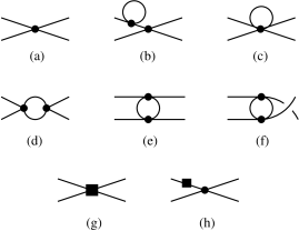
Figure 3: Classes of diagrams contributing to the PQ scattering amplitudes through NNLO. Filled circles represent vertices from ${\cal L}_{\rm LO}$ while filled squares represent vertices from ${\cal L}_{\rm NLO}$ and ${\cal L}_{\rm NNLO}$.

In this section we calculate the on-shell PQ amplitudes through NNLO. Although, as noted earlier, the PQ theory is defined in Euclidean space, we can nevertheless analytically continue the amplitudes to Minkowski momenta and set them on shell. It turns out that it is these on-shell amplitudes which appear in the coefficient of $t$ in the ratios of Fig. 2.

The diagrams contributing through NNLO are shown in Fig. 3. At LO, only Fig. 3(a) contributes, and leads to the following results for the on-shell amplitudes:

$$\mathcal{D}^{(0)} =2w_{6}^{\prime}$$ (23)

$$\mathcal{S}^{(0)}(s) =w_{8}^{\prime}+\frac{1}{2f^{2}}\left(2M_{0}^{2}-s\right).$$ (24)

Here, $M_{0}$ is the LO pion mass, given by

$$M_{0}^{2}=\chi+f^{2}(2w_{6}^{\prime}+w_{8}^{\prime})\,,$$ (25)

where we have introduced rescaled, dimensionless LECs

$$w_{k}^{\prime}=\frac{16\hat{a}^{2}W_{k}^{\prime}}{f^{4}}\hskip 10.0ptk=6,7,8.$$ (26)

Note that, because all quarks and ghosts are degenerate, all pions have the same mass, whatever their composition.

Combining Eqs. (23) and (24) according to (14) and using the on-shell result $s+t+u=4M_{0}^{2}$, we find

$$\mathcal{A}^{(0)}(s)=\frac{s-M_{0}^{2}}{f^{2}}+2w_{6}^{\prime}+w_{8}^{\prime}\,.$$ (27)

This agrees with the result of Ref. Aoki et al. (2008).

We now turn to higher-order contributions, considering first the loop graphs of NNLO and then turning to the analytic contributions of NLO and NNLO. Non-analytic contributions to mass and wavefunction renormalization arise from the “tadpole” diagrams exemplified by Fig. 3(b). Including the results from these diagrams (and also the analytic analogs in Fig. 3(h)), the form of the valence-valence propagator near the physical pole is

$$\langle\pi_{ij}(p)\pi_{ji}(-p)\rangle\sim\frac{1}{(1+\delta z)(p^{2}+M_{\pi}^{2})}\,,$$ (28)

with $\sim$ indicating that the two sides differ by terms regular at the pole. This expression defines both the wave function renormalization $\delta z$ and the physical mass $M_{\pi}$. It is further convenient to define $M_{\pi}^{2}=M_{0}^{2}+\delta M^{2}$.

Evaluating the tadpole diagrams we find

$$\delta M_{loop}^{2} =\left[\frac{1}{2}M_{0}^{2}-\frac{5}{2}f^{2}(2w_{6}^{\prime}+w_{8}^{\prime})\right]I_{1}$$ (29)

$$\delta z_{loop} =-\frac{2}{3}I_{1}\,,$$ (30)

where

$$I_{1}=\frac{1}{f^{2}}\int_{q}\frac{1}{q^{2}+M_{0}^{2}}\rightarrow\frac{M_{0}^{2}}{16\pi^{2}f^{2}}\log\left(M_{0}^{2}/\mu^{2}\right)$$ (31)

is the standard tadpole integral. Here

$$\int_{q}=\mu^{\varepsilon}\int\frac{d^{4-\varepsilon}q}{(2\pi)^{4-\varepsilon}}$$ (32)

and the arrow indicates evaluation in a modified minimal subtraction scheme ($\overline{MS}$) in which $\gamma_{E}-\log(4\pi)-1$ is subtracted along with the pole Gasser and Leutwyler (1984).

The result for $\delta M_{loop}^{2}$ is the same for all pions (as required by the graded symmetry group) including the physical, unquenched pions. It must thus contain discretization errors proportional to the combination $2w_{6}^{\prime}+w_{8}^{\prime}$, as we see is the case. The result (29) agrees with that given in Ref. Aoki et al. (2008).

Non-analytic contributions to the scattering amplitudes arise from the diagrams of Fig. 3(c-f), from wavefunction renormalization, and also from mass renormalization. The latter contribution is, at the order we work, only present in ${\cal S}$, and arises kinematically from the LO result. To see this explicitly note that the general, off-shell form of the LO amplitude is

$$\mathcal{S}^{(0)}_{\mathrm{off}}(s,t,u)=w_{8}^{\prime}+\frac{1}{6f^{2}}\left(2M_{0}^{2}-2s+t+u\right)\,.$$ (33)

When going on shell one sets $p^{2}=k^{2}=p^{\prime 2}=k^{\prime 2}$ to $-M_{\pi}^{2}$, with $M_{\pi}$ the pion mass at the order being calculated. This implies that $s+t+u=4(M_{0}^{2}+\delta M^{2})$. Substituting this in (33) one finds a NNLO contribution to ${\cal S}$ of

$$\mathcal{S}^{(2)}_{\delta M^{2}}=\frac{2\delta M^{2}}{3f^{2}}\,.$$ (34)

Combining this with the other loop contributions we find that the entire one-loop contribution to the PQ amplitudes is

$$\begin{split}\mathcal{D}^{(2)}_{loop}(s,t,u)&=-2\delta z_{loop}\mathcal{D}^{(0)}+\frac{2M_{0}^{2}}{9f^{2}}I_{1}\\ &+(1/36)\left[I_{6}(s)+I_{6}(t)+I_{6}(u)\right]\\ &+\left[-(10/3)w_{6}^{\prime}-2w_{8}^{\prime}+2w_{7}^{\prime}\right]I_{1}\\ &-(4/3)w_{6}^{\prime}I_{4}(t)\\ &+(1/3)\widetilde{w}_{8}^{\prime}\left[I_{4}(s)+I_{4}(u)-2I_{4}(t)\right]\\ &+w_{6}^{\prime 2}\left[4I_{2}(s)+4I_{2}(u)+14I_{2}(t)\right]\\ &+10w_{6}^{\prime}\widetilde{w}_{8}^{\prime}I_{2}(t)\\ &+\widetilde{w}_{8}^{\prime 2}\left[I_{2}(s)+I_{2}(u)+(17/2)I_{2}(t)\right]\end{split}$$ (35)

and

$$\begin{split}\mathcal{S}^{(2)}_{loop}(s,t,u)&=\frac{2}{3f^{2}}\delta M_{loop}^{2}-2\delta z_{loop}\mathcal{S}^{(0)}(s)\\ &+\frac{10s-13M_{0}^{2}}{18f^{2}}I_{1}\\ &+(1/18)\left[I_{7}(t,u)+I_{7}(u,t)\right]\\ &-\left[(11/3)w_{6}^{\prime}+(3/2)w_{8}^{\prime}+2w_{7}^{\prime}\right]I_{1}\\ &+(1/3)w_{6}^{\prime}\left[2I_{4}(s)-I_{4}(t)-I_{4}(u)\right]\\ &-(1/3)\widetilde{w}_{8}^{\prime}\left[I_{4}(t)+I_{4}(u)\right]\\ &+4w_{6}^{\prime}\widetilde{w}_{8}^{\prime}\left[I_{2}(s)+I_{2}(t)+I_{2}(u)\right]\\ &-(5/2)\widetilde{w}_{8}^{\prime 2}\left[I_{2}(t)+I_{2}(u)\right]\,,\end{split}$$ (36)

where

$$\widetilde{w}_{8}^{\prime}=w_{8}^{\prime}+\frac{M_{0}^{2}}{3f^{2}}\,.$$ (37)

In each case, the results proportional to $I_{1}$ are from the tadpole diagram, Fig. 3(c).

The new integrals that appear, and their values after subtraction and going on-shell, are

$$\begin{split}I_{2}(s)&=\int_{q}\frac{1}{(q^{2}+M_{0}^{2})(\widetilde{q}^{2}+M_{0}^{2})}\\ &\rightarrow\frac{1}{16\pi^{2}}\left[F(s)+1-\log(M_{0}^{2}/\mu^{2})\right]\end{split}$$ (38)

$$\begin{split}I_{4}(s)&=\frac{1}{f^{2}}\int_{q}\frac{-5s+t+u-2q^{2}-2\widetilde{q}^{2}}{2(q^{2}+M_{0}^{2})(\widetilde{q}^{2}+M_{0}^{2})}\\ &\rightarrow I_{2}(s)\frac{4M_{0}^{2}-3s}{f^{2}}-2I_{1}\end{split}$$ (39)

$$\begin{split}I_{6}(s)&=\frac{1}{f^{4}}\int_{q}(3s+p^{2}+k^{2}+q^{2}+\widetilde{q}^{2})\\ &\times\frac{(3s+p^{\prime 2}+k^{\prime 2}+q^{2}+\widetilde{q}^{2})}{(q^{2}+M_{0}^{2})(\widetilde{q}^{2}+M_{0}^{2})}\\ &\rightarrow I_{2}(s)\frac{(3s-4M_{0}^{2})^{2}}{f^{4}}+I_{1}\frac{10s-16M_{0}^{2}}{f^{2}}\end{split}$$ (40)

$$\begin{split}I_{7}(s,u)&=\frac{1}{f^{4}}\int_{q}(3(p+q)^{2}-p^{2}-k^{2}-q^{2}-\widetilde{q}^{2})\\ &\times\frac{(3(k^{\prime}+q)^{2}-p^{\prime 2}-k^{\prime 2}-q^{2}-\widetilde{q}^{2})}{(q^{2}+M_{0}^{2})(\widetilde{q}^{2}+M_{0}^{2})}\\ &\rightarrow I_{2}(s)\frac{3s^{2}+3us/2-12M_{0}^{2}s-6M_{0}^{2}u+16M_{0}^{4}}{f^{4}}\\ &+I_{1}\frac{4s+3u-10M_{0}^{2}}{f^{2}}+\frac{(6M_{0}^{2}-s)(4M_{0}^{2}-s-2u)}{32\pi^{2}f^{4}}\,,\end{split}$$ (41)

where $\widetilde{q}=q+p+k$. Thus all integrals can be written in terms of $I_{1}$ and a function defined in Ref. Aoki et al. (2008):

$$F(s)=-\sigma_{s}\log\frac{\sigma_{s}+1}{\sigma_{s}-1},\ \ \sigma_{s}=\sqrt{1-\frac{4M_{0}^{2}}{s}}\,.$$ (42)

The analytic contributions of NLO and NNLO arise from Figs. 3(g) and (h). For the mass shift and wavefunction renormalization we find

$$\begin{split}\delta M_{an}^{2}&=-(1/2)(2w_{4}+w_{5})M_{0}^{2}+(2w_{6}+w_{8})\chi\\ &{}-(1/2)(2\xi_{4}+\xi_{5})M_{0}^{2}+(2\xi_{6}+\xi_{8})\chi\\ &{}+\delta M_{ad}^{2}\end{split}$$ (43)

$$\delta z_{an} =(1/2)\left[(2w_{4}+w_{5})+(2\xi_{4}+\xi_{5})\right]+\delta z_{ad}\,,$$ (44)

where

$$w_{k}=\frac{16\hat{a}W_{k}}{f^{2}}\qquad\xi_{k}=\frac{16L_{k}\chi}{f^{2}}\qquad(k=4-8)$$ (45)

are defined in analogy with Eq. (26). $\delta M_{ad}^{2}$ and $\delta z_{ad}$ are the contributions from the “additional” terms, meaning $a^{3}$, $a^{2}m$, $a^{4}$ and $a^{2}p^{2}$ terms. They are given in Appendix A.

Incorporating the corrections from $\delta M_{an}^{2}$ and $\delta z_{an}$ we determine the NLO and NNLO analytic terms in the PQ amplitudes to have the explicit form

$$\begin{split}\mathcal{D}^{(1,2)}_{an}(s,t,u)&=(2w_{4}+w_{5})(-2w^{\prime}_{6})+w_{4}G(t)\\ &+2\chi w_{6}/f^{2}\\ &+8L_{1}G(t)^{2}+4L_{2}\left(G(s)^{2}+G(u)^{2}\right)\\ &-4L_{PQ}\left(G(s)^{2}+G(t)^{2}+G(u)^{2}\right)\\ &+(2\xi_{4}+\xi_{5})(-2w_{6}^{\prime})+\xi_{4}G(t)\\ &+2\chi\xi_{6}/f^{2}+\mathcal{D}_{ad}(t)\,,\end{split}$$ (46)

$$\begin{split}\mathcal{S}^{(1,2)}_{an}(s,t,u)&=(2w_{4}+w_{5})(-w_{8}^{\prime}-M_{0}^{2}/f^{2})\\ &+w_{4}s/(2f^{2})\\ &+2\chi(w_{6}+w_{8})/f^{2}\\ &+2L_{3}\left(G(t)^{2}+G(u)^{2}\right)\\ &+4L_{PQ}\left(G(s)^{2}+G(t)^{2}+G(u)^{2}\right)\\ &+(2\xi_{4}+\xi_{5})(-w_{8}^{\prime}-M_{0}^{2}/f^{2})\\ &+\xi_{4}s/(2f^{2})\\ &+2\chi(\xi_{6}+\xi_{8})/f^{2}+\mathcal{S}_{ad}(s)\,,\end{split}$$ (47)

where

$$G(s)=\frac{s-2M_{0}^{2}}{f^{2}}$$ (48)

and $\mathcal{D}_{ad}(t)$ and $\mathcal{S}_{ad}(s)$ are given in Appendix A. Note that, due to the great number of LECs, the analytic parts of the PQ amplitudes are poorly constrained.

The final results are obtained by combining Eqs. (23), (35) and (46) for

$${\cal D}(s,t,u)={\cal D}^{(0)}+{\cal D}^{(2)}_{loop}(s,t,u)+{\cal D}^{(1,2)}_{an}(s,t,u),$$ (49)

and similarly combining Eqs. (24), (36) and (47) for

$${\cal S}(s,t,u)={\cal S}^{(0)}(s)+{\cal S}^{(2)}_{loop}(s,t,u)+{\cal S}^{(1,2)}_{an}(s,t,u).$$ (50)

These may then be used in Eq. (14) to find $\mathcal{A}$. We find complete agreement with the result of Ref. Aoki et al. (2008). An interesting aspect of this comparison is that the terms linear in $a$ in ${\cal D}$ and ${\cal S}$ (which have the generic form $aM_{0}^{2}$ and $as$) cancel in ${\cal A}$. This is only true when the leading order amplitude ${\cal A}^{(0)}$ is expressed in terms of $M_{0}$ as in Eq (27).

IV Finite Volume Correlation Functions

In this section we calculate, in PQWChPT, the correlation functions appearing in the ratios shown schematically in Fig. 2. Specifically, we consider a cubic spatial box of length $L$ with periodic boundary conditions, and assume that the time direction satisfies $L_{t}\gg L$ and is effectively infinite. Since the PQ theory does not have a positive transfer matrix, correlation functions cannot be analyzed by inserting complete sets of states with positive norm. Furthermore, the scattering amplitudes of the infinite volume theory are not unitary. Because of these unphysical features, the standard relation due to Lüscher between finite volume energy shifts and phase shifts Luscher (1986) does not hold—neither energy shifts nor phase shifts can be defined. Instead, if one wants to “measure” scattering amplitudes, one can compare results for Euclidean correlation functions (obtained using lattice methods) with the predictions of PQWChPT. Then the unphysical features of the underlying theory are matched by those of the effective theory. This strategy was introduced in Ref. Bernard and Golterman (1996) to study pion scattering in the quenched approximation.

To approach infinite-volume scattering as closely as possible, we consider external pion fields with definite three-momentum, leaving only their time coordinates untransformed. We additionally restrict ourselves to the simplest case of pions at rest. Specifically, we calculate the following four-point correlators:

$$C_{\mathcal{D}}(t) =\langle\widetilde{\pi}_{12}(t)\widetilde{\pi}_{34}(t)\widetilde{\pi}_{21}(0)\widetilde{\pi}_{43}(0)\rangle$$ (51)

$$C_{\mathcal{S}}(t) =\langle\widetilde{\pi}_{12}(t)\widetilde{\pi}_{34}(t)\widetilde{\pi}_{23}(0)\widetilde{\pi}_{41}(0)\rangle\,,$$ (52)

with

$$\widetilde{\pi}(t)=\int_{L^{3}}d^{3}x\,\pi(\vec{x},t)\,.$$ (53)

The subscript on the integral indicates integration over finite volume. These correlation functions are, roughly speaking, the finite-volume analogs of the infinite-volume unamputated scattering amplitudes. In order to more directly access these amplitudes, we take the ratio of these correlators to the square of a single-pion correlator, which is, roughly speaking, the analog of amputation:

$$R_{\mathcal{D},\mathcal{S}}(t) =\frac{C_{\mathcal{D},\mathcal{S}}(t)}{C_{\pi}(t)^{2}}$$ (54)

$$C_{\pi}(t) =\langle\widetilde{\pi}_{12}(t)\widetilde{\pi}_{21}(0)\rangle\,.$$ (55)

These are the ratios shown schematically in Fig. 2. In this note we will always take $t$ to be positive.

It is instructive to make contact with the more familiar results in a physical (i.e. unquenched) theory. Adapting Eq. (12) to finite volume, we find that the $\pi^{+}\pi^{+}$ correlation function is related to our PQ correlators in a simple way:

$$\begin{split}C_{\pi^{+}}(t)&=\langle\widetilde{\pi}^{+}(t)\widetilde{\pi}^{+}(t)\widetilde{\pi}^{-}(0)\widetilde{\pi}^{-}(0)\rangle\\ &=2C_{\mathcal{D}}(t)+2C_{\mathcal{S}}(t)\,.\end{split}$$ (56)

It follows that

$$R_{\mathcal{D}}(t)+R_{\mathcal{S}}(t)=Ze^{-(E_{\pi^{+}\pi^{+}}-2M_{\pi})t}+{\rm exp.\ supp.,}$$ (57)

where $E_{\pi^{+}\pi^{+}}$ is the energy of the lightest $\pi^{+}\pi^{+}$ state with zero total spatial momentum, and the exponentially suppressed terms come from states with higher energies. At LO in WChPT one finds (as we will show below) that the overlap factor $Z$ is unity, so that

$$\begin{split}R_{\cal D}(t)+R_{\cal S}(t)&\approx 1-\delta Et\\ \delta E&=E_{\pi^{+}\pi^{+}}-2M_{\pi}\,.\end{split}$$ (58)

This approximation is valid as long as $t$ is large enough that the exponentially suppressed terms are negligible but also small enough that the linear term dominates the Taylor expansion of the leading exponential.

Lüscher’s result relates this shift to the infinite volume $\pi^{+}$ scattering amplitude at threshold Luscher (1986):

$$\delta E = -{\cal A}_{\pi^{+}}^{\rm th}\frac{1}{4M_{\pi}^{2}L^{3}}\left[1+c_{1}{\cal A}_{\pi^{+}}^{\rm th}\frac{1}{16\pi M_{\pi}L}+O(1/L^{2})\right]$$ (59)

$$+{\cal O}(e^{-M_{\pi}L})\,,$$

where $c_{1}=-2.837297$ is a numerical constant. The form of the $1/L^{2}$ correction, and some higher order terms, are known Luscher (1986), but we do not show them as we will not control the corresponding terms in our calculation. Note also the presence of exponentially suppressed finite-volume corrections.

Although the PQ ratios $R_{\cal D}(t)$ and $R_{\cal S}(t)$ do not behave as a sum of exponentials, what we can take over from the analysis of $R_{\pi^{+}}(t)$ is that it is useful to determine the coefficient of the term linear in $t$. In the remainder of this section we determine the PQWChPT prediction for the linear terms in $R_{\cal D}(t)$ and $R_{\cal S}(t)$. We work to NNLO in the momentum power counting of Eq. (8) and do so controlling not only the leading $1/L^{3}$ terms but also the $1/L^{4}$ corrections. We can also control a subset of the finite volume corrections proportional to $e^{-M_{\pi}L}$, but will not do so systematically.

The PQWChPT diagrams which contribute to the order we work are shown in Fig. 4. These are the same diagrams as for the infinite-volume amplitudes, Fig. 3, except for the addition of the disconnected diagrams (a-c). Our description of the calculation is broken into three subsections: leading-order results, analytic NLO and NNLO contributions, and NNLO results from loop diagrams.

IV.1 Leading-order Results

Figure 4: Classes of diagrams contributing to the correlators $C_{\cal D}(t)$ and $C_{\cal S}(t)$ in ChPT. Diagrams in which initial or final pions are interchanged are not shown separately. Notation for vertices as in Fig. 3.

The pion-disconnected diagram of Fig. 4(a) contributes only to $C_{\cal D}(t)$, with the result

$$C_{\cal D}^{({\rm disc})}(t)=C_{\pi}(t)^{2}$$ (60)

$$C_{\pi}(t)=\frac{L^{3}}{2M_{0}}e^{-M_{0}t}$$ (61)

and thus

$$R_{\cal D}^{({\rm disc})}(t)=1\,,\quad R_{\cal S}^{({\rm disc})}(t)=0\,.\quad$$ (62)

The factor of $L^{3}$ in $C_{\pi}(t)$ arises because both ends of the propagators are integrated over space. Note that, within WChPT, there are no explicit contributions from excited pions at any order. The effect of these states appears through contact terms proportional to $\delta(t)$, which arise first at NNLO. Since we always consider $t$ large enough to remove terms which are exponentially suppressed, we need not include such contact terms.

The tree-level, pion-connected diagram, Fig. 4(d), contributes to both $C_{\cal D}$ and $C_{\cal S}$. Because the four pion sources have $\vec{p}=0$, only pions at rest contribute. Thus the pion propagators attaching to the vertex are either

$$\frac{e^{-M_{0}|t_{1}|}}{2M_{0}}\ \ {\rm or}\ \ \frac{e^{-M_{0}|t-t_{1}|}}{2M_{0}}\,,$$ (63)

where $t_{1}$ is the time of the vertex. These propagators have no factors of $L^{3}$ since only one end is integrated over space. There is, however, a factor of $L^{3}$ from integrating the position of the vertex over space.

The correlator $C_{\cal D}(t)$ is the simplest to consider, because the LO vertex comes only from the $W^{\prime}_{6}$ term in ${\cal L}_{\rm LO}$ [see Eq. (15)] and therefore contains no derivatives. Based on the discussion above, we find (recalling that $t$ is positive)

$$C_{\cal D}^{({\rm conn},0)}(t) =2w_{6}^{\prime}L^{3}\int dt_{1}\frac{e^{-2M_{0}|t_{1}|}e^{-2M_{0}|t-t_{1}|}}{(2M_{0})^{4}}$$ (64)

$$=2w_{6}^{\prime}L^{3}\frac{e^{-2M_{0}t}}{(2M_{0})^{4}}\left(\frac{1}{2M_{0}}+t\right)\,.$$ (65)

The factor of $t$ arises from the region $0\leq t_{1}\leq t$ in which the vertex lies between the two sources. The $t$-independent terms come from $t_{1}<0$ and $t_{1}>t$, where the contribution drops exponentially.

At this point, it is useful to incorporate a result from the calculation of subleading orders. The diagrams which correct pion propagators, Figs. 4(b), (c), (e) and (f), form part of the geometric series which changes

$$\frac{e^{-M_{0}|t|}}{2M_{0}}\ \ {\rm to}\ \ Z_{\pi}\frac{e^{-M_{\pi}|t|}}{2M_{\pi}}\,.$$ (66)

Here $M_{\pi}$ is the physical pion mass to the order we are working, and $Z_{\pi}=1-\delta z$ is the wavefunction renormalization. For the moment we incorporate only the mass-shift, returning to the effect of $Z_{\pi}\neq 1$ below. Using the new propagators in both numerator and denominator of the ratio $R_{\cal D}(t)$, we find

$$R_{\cal D}^{({\rm conn},0)}(t) = \frac{1}{4M_{\pi}^{2}L^{3}}\left(\frac{1}{2M_{\pi}}+t\right)2w_{6}^{\prime}\,,$$ (67)

$$= \frac{1}{4M_{\pi}^{2}L^{3}}\left(\frac{1}{2M_{\pi}}+t\right){\cal D}^{(0)}\,.$$ (68)

The utility of the ratio is that the overall exponentials cancel—as noted above, this corresponds to amputation in a continuum calculation. The physical interpretation of the $t$ term is that the pions can interact at any intermediate time, while the $1/L^{3}$ suppression arises because the zero-momentum pions must overlap in order to interact. As shown in the second line, the coefficient of $t$ is, aside from the kinematical factor $1/(4M_{\pi}^{2}L^{3})$, the LO PQ scattering amplitude. This, together with the disconnected contribution from (62), gives the result (1) quoted in the introduction.

A similar analysis holds for $R_{\cal S}(t)$, except that we must now deal with the momentum dependence arising from the kinetic term in the LO Lagrangian (15). If one evaluates the diagram in position space, the derivatives in the vertex act on the pion propagators of Eq. (63) (with $M_{0}\to M_{\pi}$). Thus only time derivatives contribute, and they yield $\pm M_{\pi}$. Consider first $0<t_{1}<t$, i.e. the vertex lying between the sources. Derivatives acting on pion propagators originating at times $0$ and $t$ then give $-M_{\pi}$ and $+M_{\pi}$, respectively. This implies that $s=4M_{\pi}^{2}$ and $t=u=0$, i.e. on-shell kinematics at threshold. For $t_{1}<0$ ($t_{1}>0$), by contrast, all derivatives give $+M_{\pi}$ ($-M_{\pi}$), and one obtains, in both cases, the amplitude at off-shell kinematics: $s=t=u=4M_{\pi}^{2}$. The final result is

$$R_{\cal S}^{({\rm conn},0)}(t) = \frac{1}{4M_{\pi}^{2}L^{3}}\Bigg{[}\frac{(w_{8}^{\prime}+{M_{0}^{2}}/{3f^{2}})}{2M_{\pi}}$$ (70)

$$\quad+\left(w_{8}^{\prime}+\frac{M_{0}^{2}-4M_{\pi}^{2}}{3f^{2}}\right)t\Bigg{]}\,,$$

$$= \frac{1}{4M_{\pi}^{2}L^{3}}\Bigg{[}\frac{1}{2M_{\pi}}{\cal S}^{(0)}_{\rm off}(4M_{\pi}^{2},4M_{\pi}^{2},4M_{\pi}^{2})$$

$$\quad+{\cal S}^{(0)}(4M_{\pi}^{2})t\Bigg{]}\,.$$

This result, together with the vanishing of the disconnected contribution, is reported in Eq. (2) of the introduction. Note that, since in (2) we are quoting a LO result, we can set $M_{0}=M_{\pi}$.

As a check on our results we consider the sum $R_{\cal D}(t)+R_{\cal S}(t)$. According to the discussion above, this should be $\approx(1-\delta Et)$, with $\delta E=-{\cal A}_{\pi^{+}}^{\rm th}/(4M_{\pi}^{2}L^{2})$ [the LO term in Eq. (59)]. We find (setting $M_{0}=M_{\pi}$)

$$R_{\cal D}^{(\rm disc)}(t)+R_{\cal D}^{({\rm conn},0)}(t)+R_{\cal S}^{({\rm conn},0)}(t)=\\ \left\{1+{\cal O}\left(\frac{1}{L^{3}}\right)+\frac{1}{4M_{\pi}^{2}L^{3}}\left(2w_{6}^{\prime}+w_{8}^{\prime}-\frac{M_{\pi}^{2}}{f^{2}}\right)t\right\}\,.$$ (71)

The coefficient of $t/(4M_{\pi}^{2}L^{3})$ is indeed the $\pi^{+}$ scattering amplitude at threshold. The $1/L^{3}$ corrections to the $t$-independent terms (which are not shown in detail) are the first correction to the $Z$-factor for the two pion state.

IV.2 Analytic NLO and NNLO contributions

Analytic NLO and NNLO contributions arise from Figs. 4(b), (e) and (g). Diagrams (b) and (e) give the analytic parts of mass and wavefunction renormalization, contributions which are identical to those in infinite volume. The effect of mass renormalization has already been discussed above. Wavefunction renormalization partly cancels in the ratios, leaving a factor of $Z_{\pi}^{2}=(1-2\delta z)$, exactly what is needed to renormalize the amplitude as in infinite volume.

The analytic contributions to the vertex, Fig. 4(g), can be analyzed by a straightforward generalization of the method used for the momentum-dependent contribution to the LO vertex in $R_{{\cal S}}$. We find

$$R_{{\cal D},an}^{(1,2)}(t) = \mathrm{const}+\frac{t}{4M_{\pi}^{2}L^{3}}\mathcal{D}_{an}^{(1,2)}(4M_{\pi}^{2},0,0)\,,$$ (72)

$$R_{{\cal S},an}^{(1,2)}(t) = \mathrm{const}+\frac{t}{4M_{\pi}^{2}L^{3}}\mathcal{S}_{an}^{(1,2)}(4M_{\pi}^{2},0,0)\,,$$ (73)

where ${\cal D}_{an}^{(1,2)}$ and ${\cal S}_{an}^{(1,2)}$ are the infinite-volume analytic contributions to the two amplitudes given in Eqs. (46) and (47). We note that, at threshold, these amplitudes are just linear combinations of $a^{3}$, $aM_{\pi}^{2}$, $a^{4}$, $a^{2}M_{\pi}^{2}$ and $M_{\pi}^{4}$ with independent coefficients. The results (72) and (73) are the natural generalizations of Eqs. (68) and (70). Note that we only keep track of the terms linear in $t$, since these are proportional to the desired PQ amplitudes at threshold. The constant terms involve off-shell amplitudes.

IV.3 NNLO results from loop diagrams

In this section we extend the calculation to the one loop diagrams which appear at NNLO, focusing on the coefficient of the terms linear and quadratic in $t$ in the ratios $R_{{\cal D},{\cal S}}(t)$. At one loop there are 3 types of contributions, which we discuss in order of increasing complexity. First, there are tadpole diagrams, shown in Fig. 4(c), (f) and (h). Second there are $t$ and $u$-channel loops, exemplified by Fig. 4(i). And, third, there are $s$-channel loops, as shown in Fig. 4(j).

IV.3.1 Tadpole diagrams

Tadpole diagrams on external legs [Figs. 4(c) and (f)] renormalize the external pion propagators, contributing to $\delta M^{2}$ and $\delta z$ as described for the analytic terms. In this case, however, there is a difference compared to infinite volume, namely that in the tadpole integral $I_{1}$ one should use the finite volume pion propagator. This gives rise to corrections which are suppressed by powers of $\exp(-M_{\pi}L)$, as can be seen by implementing the periodic boundary conditions using images. We assume such corrections are negligible.

Tadpole diagrams attached to the vertex [Fig. 4(h)] are also simple to incorporate. As long as $0<t_{1}<t$, they multiply the tree-level vertex by a factor that is independent of the vertex position, leading to the usual term linear in $t$. The coefficient of $t$ is proportional to the tadpole contributions to the threshold amplitudes, and is exactly that needed to maintain the forms of Eqs. (72) and (73), with ${\cal D}$ and ${\cal S}$ now including one-loop tadpole contributions. Again, there are exponentially suppressed volume corrections which we assume negligible.

Figure 5: Classes of diagrams contributing to the correlators $C_{{\cal D}}(t)$ and $C_{{\cal S}}(t)$, arising from $\pi^{3}$ and $\pi^{5}$ terms in the external operators. All vertices are from the LO Lagrangian.

At this stage, it is appropriate to mention that there can also be tadpoles arising on the external operators at times $0$ and $t$. This is because, in practice, if one uses a local pseudoscalar operator at the quark level, then it maps into the chiral theory at LO as $\bar{q}_{k}\gamma_{5}q_{j}(x)\to c(\Sigma-\Sigma^{\dagger})_{jk}(x)$. The constant $c$ is known but unimportant here, since it cancels in the ratios. This chiral operator expands to a term proportional to $\pi_{jk}$—the operator we have been using—but with corrections proportional to $(\pi^{3})_{jk}/f^{2}$ and $(\pi^{5})_{jk}/f^{4}$. These corrections give rise, at the order we are working, to the diagrams of Fig. 5. As we now explain, however, all of these diagrams lead to contributions subleading compared to those we are keeping.

Tadpoles associated with external operators [Figs. 5(a) and (b)] cancel in the ratios. The loop diagram of Fig. 5(c) does not give rise to a term linear in $t$ because the four propagators to the left of the vertex lead to a fall off of at least $e^{-4M_{\pi}t_{1}}$. The tree-level diagram of Fig. 5(d) also does not contribute to the coefficient of $t$—it gives a $1/L^{3}$ contribution to the constant term. The same is true for the corresponding tadpole diagram, Fig. 5(e). The only diagram in this class that does give a contribution linear in $t$ is Fig. 5(f). This arises when both pions in the loop have $\vec{q}=0$. This contribution is, however, of size $t/L^{6}$ in the ratios, and thus is subleading to the $1/L^{4}$ terms that we are aiming to control.

There are also analytic corrections to the external operators, e.g. terms proportional to $\partial^{2}\pi_{jk}$ and $a^{2}\pi_{jk}$. These lead to corrections which cancel in the ratios.

IV.3.2 $t$ and $u$-channel loops

The $t$ and $u$-channel loop diagrams have the form of Fig. 4(i). Note that, since both external pions at time $t$ are summed over all space, there is no difference between the $t$ and $u$-channel loops. In order to avoid confusion between the two uses of $t$ we will couch our discussion in terms of the $u$-channel.

Figure 4(i) gives rise to a contribution proportional to the time separation $t$ as follows. Although there are two vertices (at times $t_{1}$ and $t_{2}$), when they are pulled apart in Euclidean space there is an exponential suppression, so the dominant contributions occur when $|t_{1}-t_{2}|<1/M_{\pi}$. The loop collapses to an effective vertex, which, when integrated over the intermediate time, leads to a factor of $t$. If either of the vertices is outside of the region $0<t_{1,2}<t$, it is easy to see that one does not get a term linear in $t$.

We now turn these words into a concrete evaluation. We consider first a contribution in which both vertices have no derivatives. In infinite volume, this leads to those terms in Eqs. (35) and (36) which contain the integral $I_{2}(u)$. For definiteness, we consider the contribution to ${\cal D}^{(2)}_{loop}$ of $4w_{6}^{\prime 2}I_{2}(u)$. The corresponding contribution to the finite-volume correlator is

$$C_{\cal D}(t) \supset\frac{e^{-2M_{\pi}t}}{(2M_{\pi})^{4}}4w_{6}^{\prime 2}L^{3}\widetilde{I}_{2}(t)$$ (74)

$$\widetilde{I}_{2}(t) =\frac{1}{L^{3}}\int_{0}^{t}dt_{1}\int_{0}^{t}dt_{2}\int_{\vec{x}_{1}}\int_{\vec{x}_{2}}G_{\pi}(x_{1},x_{2})^{2}\,.$$ (75)

Here $G_{\pi}(x_{1},x_{2})$ is the Euclidean pion propagator, which is related to $C_{\pi}(t)$ by

$$C_{\pi}(t_{1}-t_{2})=\int_{\vec{x}_{1}}\int_{\vec{x}_{2}}G_{\pi}(\vec{x}_{1},t_{1};\vec{x}_{2},t_{2})\,.$$ (76)

The contribution to the ratio is

$$R_{\cal D}(t)\supset\frac{1}{4M_{\pi}^{2}L^{3}}4w_{6}^{\prime 2}\widetilde{I}_{2}(t)\,.$$ (77)

It is straightforward to evaluate $\widetilde{I}_{2}(t)$ explicitly, and one finds that it consists of a term linear in $t$ up to corrections falling as $e^{-2M_{\pi}t}$. A simple way to pick out the coefficient of $t$ is to take a time derivative and then send $t\to\infty$. In this way we arrive at

$$R_{\cal D}(t)\supset\frac{t}{4M_{\pi}^{2}L^{3}}4w_{6}^{\prime 2}\widetilde{I}_{2}^{\prime}(\infty)\,,$$ (78)

for sufficiently large $t$.

To evaluate $\widetilde{I}_{2}^{\prime}(\infty)$ we note that $\widetilde{I}_{2}(t)$ can be rewritten as

$$\widetilde{I}_{2}(t)=2\int_{0}^{t}dt_{1}\int_{0}^{t_{1}}dt_{2}\int_{\vec{x}_{2}}G_{\pi}(\vec{0},t_{1};\vec{x}_{2},t_{2})^{2}\,,$$ (79)

where we have used translation invariance and the symmetry $G_{\pi}(x,0)=G_{\pi}(0,x)$. Thus its derivative is

$$\widetilde{I}_{2}^{\prime}(t)=2\int_{0}^{t}dt_{2}\int_{\vec{x}_{2}}G_{\pi}(\vec{0},0;\vec{x}_{2},t_{2})^{2}\,.$$ (80)

Given the exponential fall-off of $G_{\pi}$, this integral asymptotes to its large $t$ value once $t\gg 1/M_{\pi}$. The factor of 2 can be traded for an extension of the integral to negative values of $t$. In this way we find

$$\widetilde{I}_{2}^{\prime}(\infty) =\int_{-\infty}^{\infty}dt_{2}\int_{\vec{x}_{2}}G_{\pi}(\vec{0},0;\vec{x}_{2},t_{2})^{2}$$ (81)

$$=\int\frac{dq_{4}}{2\pi}\frac{1}{L^{3}}\sum_{\vec{q}=2\pi\vec{n}/L}\widetilde{G}_{\pi}(q)^{2}\,,$$ (82)

where $\widetilde{G}_{\pi}$ is pion propagator in momentum space. This is simply the finite volume version of $I_{2}(u=0)=\int_{q}1/(q^{2}+M_{0}^{2})^{2}$:

$$\widetilde{I}_{2}^{\prime}(\infty)=I_{2}(u=0)+{\cal O}\left(e^{-M_{\pi}L}\right)\,,$$ (83)

where images can be used to see that the finite-volume corrections fall exponentially.

The conclusion of this analysis is that, for sufficiently large $t$ and $L$, the diagram which leads to a contribution to ${\cal D}^{(2)}_{loop}$ of $4w_{6}^{\prime 2}I_{2}(u)$ contributes to the finite-volume ratio as

$$R_{\cal D}(t)\supset\frac{t}{4M_{\pi}^{2}L^{3}}4w_{6}^{\prime 2}I_{2}(u\!=\!0)\,.$$ (84)

Thus, once again, the coefficient of $t/(4M_{\pi}^{2}L^{3})$ is the infinite-volume scattering amplitude at threshold. The same argument goes through identically for $I_{2}(u)$ contributions to ${\cal S}^{(2)}_{loop}$, and for contributions to both amplitudes proportional to $I_{2}(t)$ ($t$ here the Mandelstam variable).

A similar argument also holds for the contributions to ${\cal D}^{(2)}_{loop}$ and ${\cal S}^{(2)}_{loop}$ proportional to the integrals $I_{4}(t)$, $I_{4}(u)$, $I_{6}(t)$, $I_{6}(u)$, $I_{7}(t,s,u)$ and $I_{7}(u,s,t)$. These arise when one or both of the vertices are from the kinetic term in the Lagrangian. By similar manipulations to those above, one finds that the contribution proportional to $t$ involves exactly the integrands of the infinite volume forms (39-41), evaluated at threshold, but the spatial momentum-integrals are again replaced by finite-volume sums. The short-distance divergences are unaffected by the finiteness of the volume, so the regularization and subtractions are unchanged. Thus the manipulations relating these integrals to $I_{2}$ and $I_{1}$ go through, as always up to exponentially small volume corrections. The net effect is that the forms of Eqs. (72) and (73) are maintained, with ${\cal D}$ and ${\cal S}$ now including $t$ and $u$-channel contributions.

There is one subtlety for terms with two or more derivatives acting on the same internal propagator. To illustrate this point we define the integral

$$\widetilde{I}_{\partial^{2}}(t)=\frac{1}{L^{3}}\int_{0}^{t}dt_{1}\int_{0}^{t}dt_{2}\int_{\vec{x}_{1}}\int_{\vec{x}_{2}}\\ \times[\partial_{x_{2}}^{2}G_{\pi}(x_{1};x_{2})]G_{\pi}(x_{1};x_{2})\,.$$ (85)

Although the integrand of (85) is an even function of $x_{1}-x_{2}$, one must be careful in carrying out the manipulations which give the analog of Eq. (79). The issue is that $G_{\pi}$ has a cusp at $t_{1}=t_{2}$ and therefore the time derivatives give a delta-function: $\delta(t_{1}-t_{2})$. Carefully including the region about the delta-function, we find

$$\widetilde{I}_{\partial^{2}}(t)=\lim_{\epsilon\rightarrow 0}\int_{0}^{t}dt_{1}\left[2\int_{0}^{t_{1}-\epsilon}dt_{2}+\int_{t_{1}-\epsilon}^{t_{1}+\epsilon}dt_{2}\right]\int_{\vec{x}_{2}}\\ \times[\partial_{x_{2}}^{2}G_{\pi}(\vec{0},t_{1};\vec{x}_{2},t_{2})]G_{\pi}(\vec{0},t_{1};\vec{x}_{2},t_{2})\,.$$ (86)

We now proceed as above, taking the time derivative and sending $t\rightarrow\infty$ to deduce

$$\begin{split}\widetilde{I}^{\prime}_{\partial^{2}}(\infty)&=\lim_{\epsilon\rightarrow 0}\left[\int_{-\infty}^{\epsilon}dt_{2}+\int_{-\epsilon}^{\epsilon}dt_{2}+\int_{\epsilon}^{\infty}dt_{2}\right]\\ &\hskip 50.0pt\times\int_{\vec{x}_{2}}[\partial_{x_{2}}^{2}G_{\pi}(0;x_{2})]G_{\pi}(0;x_{2})\end{split}$$ (87)

$$=\int d^{4}x_{2}[\partial_{x_{2}}^{2}G_{\pi}(0;x_{2})]G_{\pi}(0;x_{2})\,.$$ (88)

As above, we are left with a single integral over all of space-time (with space finite). Note however that if the middle integral were absent then the final equality would not hold. Proceeding from Eq. (88), it is straightforward to see that $I^{\prime}_{\partial^{2}}(\infty)$ is equal to the corresponding finite-volume amplitude at threshold.

IV.3.3 s-channel loop

The $s$-channel loop diagram is shown in Fig. 4(j). This diagram leads to the terms proportional to $I_{2}(s)$, $I_{4}(s)$ and $I_{6}(s)$ in the infinite volume amplitudes.

We begin by analyzing the case in which neither vertex has momentum dependence, which leads to the integral $I_{2}(s)$ in infinite volume. For definiteness we focus on the $\widetilde{w}_{8}^{\prime 2}I_{2}(s)$ contribution to ${\cal D}^{(2)}_{loop}$ in Eq. (35). The corresponding contribution to $C_{\cal D}(t)$ is

$$C_{\cal D}(t)\supset\\ \widetilde{w}_{8}^{\prime 2}\int_{x_{1}}\int_{x_{2}}\frac{e^{-2M_{\pi}|t_{1}|}}{(2M_{\pi})^{2}}\left[G_{\pi}(x_{1},x_{2})\right]^{2}\frac{e^{-2M_{\pi}|t-t_{2}|}}{(2M_{\pi})^{2}}\,.$$ (89)

There are many choices of the ordering of the four times $0$, $t_{1}$, $t_{2}$ and $t$, but only the four shown in Fig. 6 lead to terms linear in $t$. The others give constants or terms which fall exponentially with $t$.

Figure 6: Time-orderings of the $s$-channel loop which give rise to contributions to $R_{{\cal D},{\cal S}}(t)$ linear in $t$ at large times. The time-ordering (a) also give rise to a quadratic term, as discussed in the text.

In fact, the time ordering of Fig. 6(a) also gives a term quadratic in $t$. This occurs when both pions in the loop are at rest. The integrand is then independent of $t_{1}$ and $t_{2}$, so that the contribution to the ratio is

$$R_{\cal D}(t)\supset\widetilde{w}_{8}^{\prime 2}\left(\frac{1}{4M_{\pi}^{2}L^{3}}\right)^{2}\frac{t^{2}}{2}\,.$$ (90)

In a physical theory, this is one of the contributions which builds up the quadratic term in the expansion of $\exp(-\delta Et)$ in Eq. (57), and we will use this below as a check on our result. First, however, we determine the quadratic terms arising from the finite volume versions of the integrals $I_{4}(s)$ and $I_{6}(s)$.

These integrals have one or both vertices from the kinetic term in $\mathcal{L}_{LO}$ (Eq. (15)). For our particular kinematics the derivatives are simple to evaluate, since all pions are on-shell and at rest. The derivatives in the kinetic vertices thus give exactly the results that we obtain in infinite volume when working at threshold and on-shell ($s=4M_{\pi}^{2}$, $t=u=0$). This means that, with these substitutions, we can use Eqs. (39) and (40) to relate the finite volume versions of $I_{4}(s)$ and $I_{6}(s)$ to that of $I_{2}(s)$. The $I_{1}$ terms are to be dropped, since they arise from the $\vec{q}\neq 0$ part of the loop.

Putting this together, we find the total quadratic terms to be:

$$R_{\cal D}(t) \supset\left[\left(\widetilde{w}_{8}^{\prime}-\frac{4M_{\pi}^{2}}{3f^{2}}\right)^{2}+4w_{6}^{\prime 2}\right]\left(\frac{1}{4M_{\pi}^{2}L^{3}}\right)^{2}\frac{t^{2}}{2}$$ (91)

$$R_{\cal S}(t) \supset 4w_{6}^{\prime}\left(\widetilde{w}_{8}^{\prime}-\frac{4M_{\pi}^{2}}{3f^{2}}\right)\left(\frac{1}{4M_{\pi}^{2}L^{3}}\right)^{2}\frac{t^{2}}{2}\,.$$ (92)

Thus, if one could determine the coefficients of the quadratic terms in a simulation, one would gain additional information concerning $w_{6}^{\prime}$ and $w_{8}^{\prime}$. Note that the coefficients of the quadratic terms are not the squares of those of the linear terms give in Eqs. (67) and (70). This is another indication that the PQ theory is unphysical. The sum of the ratios is, however, physical and should be an exponential. Indeed, we find that the quadratic term in $R_{\cal D}(t)+R_{\cal S}(t)$ is exactly that needed to give the quadratic term in the expansion of Eq. (71). This provides a non-trivial check on our results.

We now return to the terms linear in $t$. We can first dispense with the time-orderings of Figs. 6(c) and (d). Here a linear term arises only when the pions in the loop have $\vec{q}=0$. This means that the contribution to $C_{{\cal D},{\cal S}}(t)$ is of order $L^{0}$ and thus that to $R_{{\cal D},{\cal S}}(t)$ is order $1/L^{6}$, which is higher order than we are controlling. The same suppression holds for the contribution of pions with $\vec{q}=0$ in time ordering of Fig. 6(b). Thus we are left to consider the $\vec{q}\neq 0$ contributions to the time-orderings of Figs. 6(a) and (b).

Using Eq. (89), the time ordering of Fig. 6(a) gives the following contribution to $R_{\cal D}(t)$:

$$R_{\cal D}(t) \supset \widetilde{w}_{8}^{\prime 2}\frac{1}{L^{6}}\int_{0}^{t}dt_{2}\int_{0}^{t_{2}}dt_{1}\int_{\vec{x}_{1}}\int_{\vec{x}_{2}}$$ (93)

$$\quad\frac{e^{-2M_{\pi}(t_{1}-t_{2})}}{(2M_{\pi})^{2}}\overline{G}_{\pi}(x_{1},x_{2})^{2}\,,$$

where the bar over the pion propagator indicates that the $\vec{q}=0$ mode has been removed. We are interested in the coefficient of $t/(4M_{\pi}^{2}L^{3})$ for large $t$, and so we again take a derivative with respect to $t$ and send $t\to\infty$. The result, after some manipulations, is $\widetilde{w}_{8}^{\prime 2}I_{a}$, with

$$I_{a}=\int_{-\infty}^{0}dt_{1}\int_{\vec{x}_{1}}e^{-2M_{\pi}t_{1}}\,\overline{G}_{\pi}(x_{1},0)^{2}\,.$$ (94)

Note that the growth of the exponential as $t_{1}$ becomes more negative is overwhelmed by the decrease in $\overline{G}_{\pi}^{2}$.

A similar calculation for the time-ordering of Fig. 6(b) yields, for the coefficient of $t/(4M_{\pi}^{2}L^{3})$, the result $\widetilde{w}_{8}^{\prime 2}I_{b}$ with

$$I_{b}=\int_{0}^{\infty}dt_{1}\int_{\vec{x}_{1}}e^{-2M_{\pi}t_{1}}\,\overline{G}_{\pi}(x_{1},0)^{2}\,.$$ (95)

Here both the exponential and the $\overline{G}_{\pi}^{2}$ factors decrease as $t_{1}$ becomes larger. Combining the two time-orderings we find $\widetilde{w}_{8}^{\prime 2}$ times

$$I_{a}+I_{b} =\int d^{4}x_{1}\;e^{-2M_{\pi}t_{1}}\bar{G}_{\pi}(x_{1},0)^{2}$$ (96)

$$=I_{2}(s=4M_{\pi}^{2})^{FV}\,.$$ (97)

As noted in the second line, this integral is the finite volume version of the corresponding infinite volume integral at threshold, expressed in position space. The factor of $\exp(-2M_{\pi}t_{1})$ simply leads to the injection of the physical threshold four-momentum through the loop.

If we could ignore the difference

$$\delta I_{2}\equiv I_{2}(s=4M_{\pi}^{2})^{FV}-I_{2}(s=4M_{\pi}^{2})\,,$$ (98)

the result (97) tells us that, in the coefficient of $t/(4M_{\pi}^{2}L^{3})$, all the NNLO corrections to ${\cal D}$ and ${\cal S}$ proportional to $I_{2}(s)$ appear exactly as in infinite volume. As we will see shortly, however, $\delta I_{2}\propto 1/L$ (plus exponentially suppressed terms) so we do need to calculate it.

First, however, we extend the calculation of the coefficient of $t$ to $s$-channel loops with momentum-dependent vertices—the loops which give rise to the integrals $I_{4}(s)$ and $I_{6}(s)$. The steps outlined above lead to the same combined integral (96), except that there are two or four derivatives acting on the various factors in the integrand. As was the case with the $u$-channel diagrams, one must carefully handle the discontinuity at $t_{1}=t_{2}$ when two derivatives act on an internal propagator. The end result, however, is still as claimed. This allows us to rewrite all contributions to the time dependent correlator which are linear in $t$ as the corresponding contributions to the finite volume threshold amplitudes. Next we may relate these to the $I_{2}(s=4M_{\pi}^{2})^{FV}$ and $I_{1}^{FV}$ using the same expressions, (39) and (40), as hold in infinite volume (with $s=4M_{\pi}^{2}$). From this follows that the difference between the finite and infinite volume forms is exponentially suppressed. Thus, aside from the $\delta I_{2}$ terms, we find that the coefficient of $t/(4M_{\pi}^{2}L^{3})$ generated by $s$-channel loop diagrams is just full infinite-volume contribution from the same diagrams evaluated at threshold.

Our final task is to evaluate $\delta I_{2}$. Standard manipulations lead to the following expression

$$\delta I_{2}=\left[\frac{1}{L^{3}}\sum_{\vec{q}\neq 0}-\int\frac{d^{3}q}{(2\pi)^{3}}\right]\frac{1}{4E_{\vec{q}}\,[\vec{q}\,]^{2}}\,,$$ (99)

where $E_{\vec{q}}=\sqrt{[\vec{q}\,]^{2}+M_{\pi}^{2}}$. Since the UV divergences cancel in the difference between sum and integral, we can introduce a regulator term $\exp(-\alpha[\vec{q}\,]^{2})$, as long as we send $\alpha\to 0^{+}$. With this regulator in place, we can use Lüscher’s summation formula Luscher (1986) (in the particular form quoted in Ref. Bernard and Golterman (1996))

$$\left[\frac{1}{L^{3}}\sum_{\vec{q}\neq 0}-\int\frac{d^{3}q}{(2\pi)^{3}}\right]\frac{f(\vec{q}^{2})}{\vec{q}^{2}}=\frac{c_{1}f(0)}{4\pi L}-\frac{f^{\prime}(0)}{L^{3}}\,,$$ (100)

where $c_{1}$ is the constant given after Eq. (59). This result is valid up to exponentially small corrections as long as $f$ and all its partial derivatives are square integrable (as is the case with our regularized sum). Applying this result, we find

$$\delta I_{2}=\frac{c_{1}}{16\pi M_{\pi}L}+\frac{1}{8(M_{\pi}L)^{3}}\,.$$ (101)

At the order we are working, we need keep only the $1/L$ term.

Collecting all the $1/L$ terms, we find their contribution to the ratios to be:

$$R_{\cal D}(t) \supset\left[\left(\widetilde{w}_{8}^{\prime}-\frac{4M_{\pi}^{2}}{3f^{2}}\right)^{2}\!\!\!+4w_{6}^{\prime 2}\right]\!\frac{1}{4M_{\pi}^{2}L^{3}}\frac{c_{1}t}{16\pi M_{\pi}L}$$ (102)

$$R_{\cal S}(t) \supset 4w_{6}^{\prime}\left(\widetilde{w}_{8}^{\prime}-\frac{4M_{\pi}^{2}}{3f^{2}}\right)\frac{1}{4M_{\pi}^{2}L^{3}}\frac{c_{1}t}{16\pi M_{\pi}L}\,.$$ (103)

The combinations of LECs here are the same as in the $t^{2}$ terms, Eqs. (91) and (92), because the both arise from the $I_{2}(s)$ integral in finite volume.

A check on this result is that the $t/L^{4}$ term in the $\pi^{+}\pi^{+}$ correlator $R_{\cal D}(t)+R_{\cal S}(t)$ agrees with that obtained with Lüscher’s general formula (59).

IV.4 Summary of results

Collecting the results from this and the previous section, we find

$$\begin{split}R_{\cal D}(t)&=1+{\cal O}\left(\frac{M_{\pi}^{2}}{f^{2}}\frac{1}{M_{\pi}^{3}L^{3}}\right)+\frac{t}{4M_{\pi}^{2}L^{3}}{\cal D}(4M_{\pi}^{2},0,0)\\ &+\left[\left(\widetilde{w}_{8}^{\prime}-\frac{4M_{\pi}^{2}}{3f^{2}}\right)^{2}+4w_{6}^{\prime 2}\right]\\ &\hskip 20.0pt\times\left\{\frac{1}{4M_{\pi}^{2}L^{3}}\frac{c_{1}t}{16\pi M_{\pi}L}+\left(\frac{1}{4M_{\pi}^{2}L^{3}}\right)^{2}\frac{t^{2}}{2}\right\}\\ &\hskip 90.0pt\times\Bigg{\{}1+{\cal O}\left(\frac{M_{\pi}^{2}}{f^{2}}\frac{1}{M_{\pi}L}\right)\!\!\Bigg{\}}\\ &+{\cal O}\left(\left[\frac{M_{\pi}^{2}}{f^{2}}\frac{t}{M_{\pi}^{2}L^{3}}\right]^{3}\right)+{\cal O}(e^{-M_{\pi}L})+\textrm{exp. suppr.}\,,\end{split}$$ (104)

Here ${\cal D}$ is the full NNLO amplitude. The corresponding result for $R_{\cal S}(t)$ is

$$\begin{split}R_{\cal S}(t)&={\cal O}\left(\frac{M_{\pi}^{2}}{f^{2}}\frac{1}{M_{\pi}^{3}L^{3}}\right)+{\cal S}(4M_{\pi}^{2},0,0)\frac{t}{4M_{\pi}^{2}L^{3}}\\ &+4w_{6}^{\prime}\left(\widetilde{w}_{8}^{\prime}-\frac{4M_{\pi}^{2}}{3f^{2}}\right)\\ &\hskip 20.0pt\times\left\{\frac{1}{4M_{\pi}^{2}L^{3}}\frac{c_{1}t}{16\pi M_{\pi}L}+\left(\frac{1}{4M_{\pi}^{2}L^{3}}\right)^{2}\frac{t^{2}}{2}\right\}\\ &\hskip 90.0pt\times\Bigg{\{}1+{\cal O}\left(\frac{M_{\pi}^{2}}{f^{2}}\frac{1}{M_{\pi}L}\right)\!\!\Bigg{\}}\\ &+{\cal O}\left(\left[\frac{M_{\pi}^{2}}{f^{2}}\frac{t}{M_{\pi}^{2}L^{3}}\right]^{3}\right)+{\cal O}(e^{-M_{\pi}L})+\textrm{exp. suppr.}\,.\end{split}$$ (105)

Note that the last three lines of Eqs. (104) and (105) are identical.

Thus, if one can measure the coefficients of $t/L^{3}$, one obtains the corresponding infinite volume PQ threshold scattering amplitudes at NNLO. In fact, it is plausible that this holds to all orders, since the analysis above shows how picking out the $t$ term corresponds to LSZ reduction in infinite volume. Of course, it is non-trivial to pick out these coefficients, but our results provide the coefficients of the leading competing terms—those proportional to $t/L^{4}$ and $t^{2}/L^{6}$.

For completeness we give the PQ results for the threshold scattering amplitudes. Using the results $F(4M_{\pi}^{2})=0$, $F(0)=-2$ and the notation $Q=\log(M_{\pi}^{2}/\mu^{2})/(16\pi^{2})$ these are

$${\cal D}(4M_{\pi}^{2},0,0)=2w_{6}^{\prime}+{\cal D}^{(1,2)}_{an}(4M_{\pi}^{2},0,0)\\ +\frac{1}{16\pi^{2}}\bigg{[}-\frac{M_{\pi}^{4}}{2f^{4}}+\frac{M_{\pi}^{2}}{f^{2}}(2w_{6}^{\prime}-7w_{8}^{\prime})-14w_{6}^{\prime 2}-10w_{6}^{\prime}w_{8}^{\prime}\\ -(17/2)w_{8}^{\prime 2}\bigg{]}+Q\bigg{[}-\frac{5M_{\pi}^{4}}{2f^{4}}+\frac{M_{\pi}^{2}}{f^{2}}(4w_{6}^{\prime}+2w_{7}^{\prime}-5w_{8}^{\prime})\\ -22w_{6}^{\prime 2}-10w_{6}^{\prime}w_{8}^{\prime}-(21/2)w_{8}^{\prime 2}\bigg{]}$$ (106)

and

$${\cal S}(4M_{\pi}^{2},0,0)=w_{8}^{\prime}-\frac{M_{\pi}^{2}}{f^{2}}+{\cal S}^{(1,2)}_{an}(4M_{\pi}^{2},0,0)-\frac{\delta M_{an}^{2}}{f^{2}}\\ +\frac{1}{16\pi^{2}}\bigg{[}\frac{M_{\pi}^{4}}{f^{4}}+\frac{2M_{\pi}^{2}}{f^{2}}(-2w_{6}^{\prime}+3w_{8}^{\prime})-4w_{6}^{\prime}w_{8}^{\prime}+5w_{8}^{\prime 2}\bigg{]}\\ +Q\bigg{[}-\frac{M_{\pi}^{4}}{f^{4}}+\frac{M_{\pi}^{2}}{f^{2}}(2w_{6}^{\prime}-2w_{7}^{\prime}+8w_{8}^{\prime})\\ -12w_{6}^{\prime}w_{8}^{\prime}+5w_{8}^{\prime 2}\bigg{]}\,.$$ (107)

We do not give explicit expressions for ${\cal D}^{(1,2)}_{an}(4M_{\pi}^{2},0,0)$ and ${\cal S}^{(1,2)}_{an}(4M_{\pi}^{2},0,0)$ as they can be readily determined from Eqs. (46) and (47).

Appendix A Additional contributions to $\mathcal{D}$ and $\mathcal{S}$

In this appendix we analyze the additional contributions to the PQ amplitudes that come from the $a^{3}$ terms in the NLO Lagrangian and from the $ma^{2}$, $a^{4}$ and $p^{2}a^{2}$ terms in the NNLO. We begin by enumerating all of the $a^{3}$ terms allowed by chiral symmetry:

$$\begin{split}\mathcal{L}_{a^{3}}&\sim\hat{a}^{3}\langle\Sigma+\Sigma^{\dagger}\rangle^{3}\\ &{}+\hat{a}^{3}\langle\Sigma-\Sigma^{\dagger}\rangle^{2}\langle\Sigma+\Sigma^{\dagger}\rangle\\ &{}+\hat{a}^{3}\langle\Sigma^{2}+(\Sigma^{\dagger})^{2}\rangle\langle\Sigma+\Sigma^{\dagger}\rangle\\ &{}+\hat{a}^{3}\langle\Sigma^{2}-(\Sigma^{\dagger})^{2}\rangle\langle\Sigma-\Sigma^{\dagger}\rangle\\ &{}+\hat{a}^{3}\langle\Sigma^{3}+(\Sigma^{\dagger})^{3}\rangle\\ &{}+\hat{a}^{3}\langle\Sigma+\Sigma^{\dagger}\rangle\,.\end{split}$$ (108)

We use $\sim$ throughout this appendix to indicate that the two sides are equal with an independent LEC multiplying each term. The key observation is that these terms, when expanded in $\mathcal{\pi}$, produce $\langle\pi^{2}\rangle$, $\langle\pi^{2}\rangle^{2}$ and $\langle\pi^{4}\rangle$ with independent coefficients. The particular forms of these coefficients in terms of the unknown LECs provides no useful information.

Both the $ma^{2}$ and $a^{4}$ sectors generate the same three pion terms with independent coefficients. The argument for the $ma^{2}$ terms is identical to that for the $a^{3}$ sector, since the spurions $A$ and $\chi$ transform in the same way. For the $a^{4}$ sector we can show this result by displaying three chiral operators which give linearly independent contributions to the three pionic operators. An example is

$$\begin{split}\mathcal{L}_{a^{4}}&\sim\hat{a}^{4}\langle\Sigma+\Sigma^{\dagger}\rangle^{4}\\ &{}+\hat{a}^{4}\langle\Sigma-\Sigma^{\dagger}\rangle^{2}\langle\Sigma+\Sigma^{\dagger}\rangle^{2}\\ &{}+\hat{a}^{4}\langle\Sigma+\Sigma^{\dagger}\rangle^{2}+\cdots\,,\end{split}$$ (109)

where the dots indicate additional terms which we do not need to enumerate.

It remains to consider the $p^{2}a^{2}$ terms. Starting on the level of the pion fields, we first list all two-derivative quadratic and quartic terms. This is done without regard to chiral symmetry, using only that $\langle\pi\rangle=0$. The resulting set is

$$\begin{array}[]{c}\langle\partial_{\mu}\pi\,\partial_{\mu}\pi\rangle\\[5.0pt] \langle\partial_{\mu}\pi\,\pi\rangle\langle\partial_{\mu}\pi\,\pi\rangle\\[5.0pt] \langle\partial_{\mu}\pi\,\partial_{\mu}\pi\,\pi^{2}\rangle\\[5.0pt] \langle\partial_{\mu}\pi\,\pi\,\partial_{\mu}\pi\,\pi\rangle\\[5.0pt] \langle\partial_{\mu}\,\pi\partial_{\mu}\pi\rangle\langle\pi^{2}\rangle\,.\end{array}$$ (110)

Because this is the maximal set of pionic terms to the order we are working, it is sufficient to show that the $p^{2}a^{2}$ terms allowed by chiral symmetry produce the entire set, with independent coefficients. This is indeed the case, as follows from

$$\begin{split}\mathcal{L}_{p^{2}a^{2}}&\sim\hat{a}^{2}\left[\langle\partial_{\mu}\Sigma\rangle^{2}+\langle\partial_{\mu}\Sigma^{\dagger}\rangle^{2}\right]\\ &{}+\hat{a}^{2}\langle\partial_{\mu}\Sigma\partial_{\mu}\Sigma^{\dagger}\rangle\\ &{}+\hat{a}^{2}\langle\partial_{\mu}\Sigma\partial_{\mu}\Sigma^{\dagger}\rangle\langle\Sigma+\Sigma^{\dagger}\rangle^{2}\\ &{}+\hat{a}^{2}\langle\partial_{\mu}\Sigma\partial_{\mu}\Sigma^{\dagger}(\Sigma^{2}+(\Sigma^{\dagger})^{2})\rangle\\ &{}+\hat{a}^{2}\langle\partial_{\mu}\Sigma\partial_{\mu}\Sigma(\Sigma^{\dagger})^{2}\rangle+\cdots\,.\end{split}$$ (111)

These terms are enough to independently give the set (110).

From these results, we can determine the contribution of all $a^{3}$, $a^{2}m$, $a^{4}$ and $p^{2}a^{2}$ terms to the mass and wave function renormalizations and to the PQ amplitudes. We find

$$\delta z_{ad} \sim\hat{a}^{2}$$ (112)

$$\delta M^{2}_{ad} \sim\hat{a}^{2}M_{0}^{2}+\hat{a}^{3}+\hat{a}^{4}$$ (113)

$$\mathcal{D}_{ad}(t) \sim\hat{a}^{2}t+\hat{a}^{2}M_{0}^{2}+\hat{a}^{3}+\hat{a}^{4}-2\delta z_{ad}\mathcal{D}^{(0)}$$ (114)

$$\begin{split}\mathcal{S}_{ad}(s)&\sim\hat{a}^{2}s+\hat{a}^{2}M_{0}^{2}+\hat{a}^{3}+\hat{a}^{4}-2\delta z_{ad}\mathcal{S}^{(0)}(s)\\ &{}+2\delta M_{ad}^{2}/(3f^{2})\,.\end{split}$$ (115)

Appendix B Determining $W^{\prime}_{7}$

In this appendix we sketch a method for determining the LEC $W^{\prime}_{7}$ in which its contribution appears at tree-level. The method is by no means unique, but it is the simplest approach we have found within the context of pion scattering.

Expanding out the $W^{\prime}_{7}$ term in the LO chiral Lagrangian (15), the first non-vanishing term is

$${\cal L}_{\rm LO}\supset\frac{w^{\prime}_{7}}{18f^{2}}\langle\pi^{3}\rangle^{2}\,.$$ (116)

To get a tree-level contribution from this vertex one needs six external pions. We propose calculating the following finite-volume correlation function

$$C_{3\pi}(t)=\langle\widetilde{\pi}_{12}(0)\widetilde{\pi}_{23}(0)\widetilde{\pi}_{45}(0)\widetilde{\pi}_{31}(t)\widetilde{\pi}_{56}(t)\widetilde{\pi}_{64}(t)\rangle\,,$$ (117)

and then forming the ratio

$$R_{3\pi}(t)=\frac{C_{3\pi}(t)}{C_{\pi}(t)^{3}}\,.$$ (118)

Here $\widetilde{\pi}_{jk}$ are the $\vec{p}=0$ fields defined in Eq. (53) and the single-pion correlator $C_{\pi}(t)$ is defined in Eq. (55). The subscripts on the pion fields indicate valence flavors, of which there must be six. We consider only $t>0$ in the following.

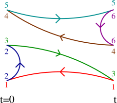
Figure 7: Quark contraction for the correlator $C_{3\pi}$ of Eq. (117).

The choice of valence fields in (117) allows only a single quark-level contraction, shown in Fig. 7. By construction, this contraction has two quark loops, in order to match with the double-strace six-pion vertex of (116). This will be a more challenging contraction to calculate in numerical simulations than those of Fig. 1, because of the “source to source” propagators at times $0$ and $t$. Nevertheless, with recent advances in calculations of “all-to-all” propagators, we expect that the calculation should be feasible.

We have written the correlator in terms of the pion fields from the chiral Lagrangian, but, as discussed in Sec. IV.3.1, in practice one would use a quark-level pseudoscalar field, $\bar{q}_{k}\gamma_{5}q_{j}$. The corresponding chiral operator is

$$(\Sigma-\Sigma^{\dagger})_{jk}=c\left[\pi_{jk}-\frac{1}{3f^{2}}(\pi^{3})_{jk}+\dots\right]\,,$$ (119)

where the constant $c$ is known but not needed. It turns out that in this calculation, unlike that in the main text, the $\pi^{3}$ part of the interpolating operator contributes at leading order to the quantities of interest. This means that it is essential for the present method to use (a discretization of) a local pseudoscalar bilinear to create the pion fields, and not, for example, a non-local operator.

Figure 8: Tree-level diagrams in PQWChPT contributing to linear or quadratic dependence in $C_{3\pi}(t)$. The flavor indices of the external fields are (implicitly) ordered as in Fig. 7. Notation for vertices as in Fig. 3.

Our choice of flavor indices significantly restricts the diagrams that can appear and the vertices that contribute. There is no pion-disconnected diagram, and the two tree-level diagrams which contribute are shown in Figs. 8(a) and (b). Note that the four-pion vertices in (b) must be attached to the external legs as shown, other possibilities being forbidden by the flavor indices. There are also contributions involving the $\pi^{3}$ and $\pi^{5}$ parts of interpolating fields, Eq. (119). For reasons explained below, the only diagrams of this type contributing to quantities of interest are those shown in Figs. 8(c-f). We stress that all six diagrams in Fig. 8 contribute at the same order in WChPT.

We begin by discussing the three-pion scattering diagram (a). Only the $w^{\prime}_{7}$ vertex in ${\cal L}_{\rm LO}$ has the $\langle\pi^{3}\rangle^{2}$ form needed to contribute. A straightforward calculation along the lines of those discussed in the main text leads to

$$R_{3\pi}(t)\Big{|}_{w^{\prime}_{7}}=-\frac{w^{\prime}_{7}}{f^{2}}\frac{1}{L^{6}(2M_{0})^{3}}\left(t+\frac{1}{3M_{0}}\right)\,.$$ (120)

The term linear in $t$ arises, as usual, because the interaction can occur at any time in the range $0-t$. The volume suppression is now $1/L^{6}$ [compared to $1/L^{3}$ for the two-pion interaction, as in Eq. (1)] because all three pions must be in contact. Note that at the order we are working in this appendix, $M_{0}$ and $M_{\pi}$ are interchangeable.

Turning now to Fig. 8(b), we find that only vertices having the pionic form $\langle\pi^{4}\rangle$ contribute. Such a form arises only from the mass, $w^{\prime}_{6}$ and $w^{\prime}_{8}$ terms in ${\cal L}_{\rm LO}$ [eq. (15)]. The kinetic term does not contribute. After a straightforward but tedious calculation, we find

$$R_{3\pi}(t)\Big{|}_{(w^{\prime}_{8})^{2}}=\frac{-9(\widetilde{w}^{\prime}_{8})^{2}}{2}\frac{1}{L^{6}(2M_{0})^{4}}$$ (121)

$$\times\left(\frac{t^{2}}{2}+\frac{t}{M_{0}}+\frac{11}{48M_{0}^{2}}+\frac{e^{-2M_{0}t}}{16M_{0}^{2}}\right)\,.$$

In the LCE regime, $w^{\prime}_{k}\sim M_{0}^{2}/f^{2}$, so the term linear in $t$ is of the same order as that in the $w^{\prime}_{7}$ contribution (120).

The quadratic term in (121) arises because of the presence of two vertices, much like the quadratic term discussed in the main text. The linear term arises both from contributions in which the two vertices are close in time and integrated together from $0-t$, and when one of the vertices is close to either $0$ or $t$. The latter origin suggests that one should also consider contributions in which one of the vertices is “absorbed” into the sources. Indeed, such diagrams, exemplified by those in Fig. 8(c-f), do contribute at the same order.

As is evident from the result (121) there are exponentially falling terms for small $t$. There are also contributions from excited states which show up in ChPT as contact terms. To avoid these, we consider henceforth only terms proportional to $t$ and $t^{2}$. It turns out that there are no other LO diagrams leading to quadratic dependence, and the only other diagrams leading to linear dependence are those of Fig. 8(c-f). Evaluating these diagrams, we find

$$R_{3\pi}(t)\Big{|}_{w^{\prime}_{8}}=6\frac{\widetilde{w}^{\prime}_{8}}{f^{2}}\frac{1}{L^{6}(2M_{0})^{3}}t+{\rm const.}\,.$$ (122)

Combining these results gives

$$R_{3\pi}(t)\supset-\frac{t^{2}}{(2M_{0})^{4}L^{6}}\frac{9(\widetilde{w}^{\prime}_{8})^{2}}{4}$$ (123)

$$-\frac{t}{(2M_{0})^{3}f^{2}L^{6}}\left[w^{\prime}_{7}-6\widetilde{w}^{\prime}_{8}+\frac{9}{4}\frac{f^{2}}{M_{0}^{2}}(\widetilde{w}^{\prime}_{8})^{2}\right]\,.$$

Higher order contributions will lead to corrections suppressed powers of $M_{\pi}/(4\pi f)$, $a$ and $1/L$. Assuming these corrections to be small, the coefficient of $t^{2}$ allows one to determine $\widetilde{w}^{\prime}_{8}$, while that of $t$ gives a combination of $w^{\prime}_{7}$ and $\widetilde{w}^{\prime}_{8}$. Alternatively, $\widetilde{w}^{\prime}_{8}$ can be determined from other quantities such as the two pion correlators discussed in the main text. Either way, given $\widetilde{w}^{\prime}_{8}$ one can use $R_{3\pi}(t)$ to determine $w^{\prime}_{7}$.

A noteworthy feature of the result (123) is that the $t^{2}$ term becomes comparable to the linear term at the relatively short time $t\sim 1/M_{0}$. This differs from the corresponding results for the two-pion correlators [Eqs. (104) and (105)] for which the quadratic term becomes important at

$$t\sim\frac{1}{M_{0}}(M_{0}L)(fL)^{2}\gg\frac{1}{M_{0}}$$ (124)

[see Eq. (5)]. The last inequality follows since one must have $M_{0}L\gg 1$ and $fL\gtrsim 1$ to avoid large finite-volume effects. The upshot of this discussion is that the quadratic term is much more important for the three-pion ratio than for the two-pion ratios. This is not true for cubic and higher order terms, which become important only at the longer times of Eq. (124).

References

Wilson (1974)K. G. Wilson, Phys.Rev., D10, 2445 (1974).
Giusti and Luscher (2009)L. Giusti and M. Lüscher, JHEP, 0903, 013 (2009), arXiv:0812.3638 [hep-lat] .
Durr et al. (2011)S. Durr, Z. Fodor,
C. Hoelbling, S. Katz, S. Krieg, et al., JHEP, 1108, 148 (2011), arXiv:1011.2711
[hep-lat] .
Baron et al. (2010)R. Baron, P. Boucaud,
J. Carbonell, A. Deuzeman, V. Drach, et al., JHEP, 1006, 111 (2010), arXiv:1004.5284
[hep-lat] .
Sharpe and Singleton (1998)S. R. Sharpe and J. Singleton, Robert L., Phys.Rev., D58, 074501 (1998), arXiv:hep-lat/9804028
[hep-lat] .