Penetration of a vortex dipole across an interface of Bose–Einstein condensates

Abstract

The dynamics of a vortex dipole in a quasi-two dimensional two-component Bose–Einstein condensate are investigated. A vortex dipole is shown to penetrate the interface between the two components when the incident velocity is sufficiently large. A vortex dipole can also disappear or disintegrate at the interface depending on its velocity and the interaction parameters.

I Introduction

Vortex rings, such as smoke rings blown from smoker’s mouth, propagate in the direction of the axis of the ring with a long lifetime. The two-dimensional (2D) analogue of a vortex ring is a vortex dipole, which consists of a pair of vortices of opposite circulations, propagating side by side. A vortex dipole is a very stable structure and carries momentum in the direction of propagation.

In superfluids, a vortex dipole consists of a pair of quantized vortices, whose circulations are quantized to $\pm h/m$ with $h$ being Planck’s constant and $m$ being an atomic mass. Such quantized vortex dipoles have been generated and observed in Bose–Einstein condensates (BECs) of atomic gases Inouye ; Neely ; Freilich ; Middel and of exciton polaritons Roumpos ; Nardin . A quantized vortex dipole propagates with velocity $\simeq\hbar/(md)$, where $d$ is the distance between vortices. In a uniform superfluid, $d$ is constant in time and a quantized vortex dipole propagates with a constant velocity. In an inhomogeneous system, on the other hand, each vortex of a vortex dipole follows its own trajectory Neely ; Freilich ; Middel or even remains stationary Freilich ; Crasovan .

In the experiment reported in Ref. Neely , a vortex dipole was generated in an oblate BEC, which propagated through the system. When a vortex dipole reached the edge of the condensate, the vortex and antivortex disintegrated and they moved along the edge of the condensate in opposite directions. This behavior is similar to that of a classical vortex dipole moving towards a rigid wall Lamb , where the vortex and antivortex disintegrate and move along the wall in opposite directions. For both a wall and the edge of a condensate, a vortex dipole cannot go beyond the boundary. In this paper, we investigate the dynamics of a vortex dipole moving towards an interface between BECs of different components. Few studies have been performed on this kind of vortex dynamics at interfaces even in classical fluids. In classical fluids, dynamics of vortex rings moving towards a density interface have been studied Linden ; Dahm ; Kuehn .

In the present paper, we will show that a vortex dipole can penetrate the interface in a two-component BEC, in which quantized vortices in one component are transferred to the other component. A vortex dipole also disappears or disintegrates at the interface. These behaviors depend on the incident velocity of the vortex dipole and the atomic scattering lengths that determine the interfacial tension and the width of the interface. For some parameters, the cores of the vortex dipole after the penetration are occupied by the other component. When only one vortex is occupied, the occupying fraction tunnels and oscillates between the vortex pair. In a trapping potential, a rich variety of vortex dynamics can be observed.

This paper is organized as follows. Section II gives a basic formalism. Section III numerically demonstrates the dynamics of vortex dipoles in an ideal system and discusses the parameter dependence of the dynamics. Section IV investigates the dynamics of vortex dipoles in a trapped BEC. Section V provides conclusions to this study.

II Formulation of the problem

We consider a two-component BEC in mean-field theory. The dynamics of the macroscopic wave functions $\psi_{1}$ and $\psi_{2}$ of components 1 and 2 are described by the Gross–Pitaevskii (GP) equation,

$$i\hbar\frac{\partial{\Psi_{1}}}{\partial t} = \left(-\frac{\hbar^{2}}{2m_{1}}\nabla^{2}+V_{1}+G_{11}|\Psi_{1}|^{2}+G_{12}|\Psi_{2}|^{2}\right)\Psi_{1},$$

$$i\hbar\frac{\partial{\Psi_{2}}}{\partial t} = \left(-\frac{\hbar^{2}}{2m_{2}}\nabla^{2}+V_{2}+G_{22}|\Psi_{2}|^{2}+G_{12}|\Psi_{1}|^{2}\right)\Psi_{2},$$

where $m_{j}$ is an atomic mass, $V_{j}$ is an external potential, and $G_{jj^{\prime}}=2\pi\hbar^{2}a_{jj^{\prime}}(m_{j}^{-1}+m_{j^{\prime}}^{-1})$ with $a_{jj^{\prime}}$ being the $s$-wave scattering lengths between atoms in components $j$ and $j^{\prime}$ ($j,j^{\prime}=1,2$). The wave function is normalized as $\int|\Psi_{j}|^{2}d\bm{r}=N_{j}$, where $N_{j}$ is the number of atoms in component $j$.

For simplicity, we restrict ourselves to quasi-2D systems in the following analysis. The system is assumed to be tightly confined in the $z$ direction by a potential $V_{zj}(z)$ and the wave function is reduced to the form $\Psi_{j}(\bm{r})=\phi_{j}(z)\psi_{j}(x,y)$, where $\phi_{j}(z)$ is the normalized wave function of the ground state for the potential $V_{zj}(z)$. Multiplying $\phi_{j}(z)$ to Eq. (1) and integrating it with respect to z, we have the effective 2D GP equation,

$$i\hbar\frac{\partial{\psi_{1}}}{\partial t} = \left(-\frac{\hbar^{2}}{2m_{1}}\nabla_{\perp}^{2}+V_{\perp 1}+g_{11}|\psi_{1}|^{2}+g_{12}|\psi_{2}|^{2}\right)\psi_{1},$$

$$i\hbar\frac{\partial{\psi_{2}}}{\partial t} = \left(-\frac{\hbar^{2}}{2m_{2}}\nabla_{\perp}^{2}+V_{\perp 2}+g_{22}|\psi_{2}|^{2}+g_{12}|\psi_{1}|^{2}\right)\psi_{2},$$

where $\nabla_{\perp}^{2}$ is the 2D Laplacian, $V_{\perp j}(x,y)=V_{j}(\bm{r})-V_{zj}(z)$, and

$$g_{jj^{\prime}}=G_{jj^{\prime}}\int|\phi_{j}|^{2}|\phi_{j^{\prime}}|^{2}dz.$$ (3)

We assume that the interaction parameters $g_{jj^{\prime}}$ satisfy the immiscible condition,

$$g_{11}g_{22}<g_{12}^{2}.$$ (4)

We solve the effective 2D GP equation (2) numerically. The initial state is the ground state obtained by the imaginary-time propagation of Eq. (2), i.e., $i$ in the left-hand sides of Eq. (2) is replaced with $-1$. The imaginary- and real-time propagations are obtained using the pseudospectral method Recipes . The computational size is large enough that the boundary condition does not affect the results.

III Dynamics of vortex dipoles in an ideal system

We first consider an ideal system to study the dynamics of vortex dipoles, where the trapping potential is absent and the interface between the two components is straight along the $y$ axis. For simplicity, we assume $m_{1}=m_{2}$ and $g_{11}=g_{22}\equiv g$. The width of the interface is characterized by the parameter

$$\Delta\equiv\frac{g_{12}}{g}-1.$$ (5)

For $0<\Delta\ll 1$, the density distribution with the boundary condition $\lim_{x\rightarrow-\infty}n_{1}=\lim_{x\rightarrow\infty}n_{2}=n_{0}$ is given by Barankov

$$n_{j}(x)\simeq\frac{n_{0}}{2}\left[1+(-1)^{j}\tanh\frac{\sqrt{2\Delta}x}{\xi}\right],$$ (6)

where $n_{0}$ is the density far from the interface and $\xi=\hbar/(mgn_{0})^{1/2}$ is the healing length. The width of the interface $w$ is thus proportional to $\xi/\sqrt{\Delta}$. The time is normalized as $\tilde{t}=tv_{\rm s}/\xi$, where $v_{\rm s}=(gn_{0}/m)^{1/2}$ is the sound velocity.

A vortex dipole is generated by the method proposed in Ref. Aioi (see Fig. 3 in Ref. Aioi ). When an attractive Gaussian potential produced by a red-detuned laser beam is displaced in a quasi-2D BEC, a vortex dipole is created in front of the potential and “launched” in the direction of the displacement Aioi . We create a vortex dipole in component 1 using a Gaussian potential with magnitude $V_{0}>0$ and width $w$ as

$$V_{\perp 1}=V_{\rm G}\equiv-V_{0}\exp\left\{-\frac{[\bm{r}-\bm{r}_{0}(t)]^{2}}{w^{2}}\right\}.$$ (7)

The position $\bm{r}_{0}(t)$ is linearly displaced between the times $t=0$ and $t=T$, and a vortex dipole is launched from the potential towards the direction of $\bm{r}_{0}(T)-\bm{r}_{0}(0)$. The velocity of a vortex dipole can be controlled by the parameters $V_{0}$, $w$, and the function $\bm{r}_{0}(t)$. The Gaussian potential is located far from the interface, and its motion does not affect the dynamics near the interface. The dynamics of a vortex dipole therefore depend only on its velocity and not on each parameter in Eq. (7).

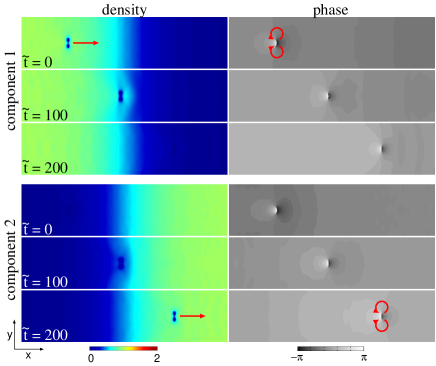
Figure 1: (Color online) Dynamics of normalized density profiles $|\psi_{j}|^{2}/n_{0}$ and phase profiles ${\rm arg}\,\psi_{j}$ for $g_{11}=g_{22}$ and $\Delta=g_{12}/g_{11}-1=10^{-3}$. The velocity of the incident vortex dipole is $v_{\rm in}=0.31v_{\rm s}$, where $v_{\rm s}$ is the sound velocity. The direction of the vortex dipole propagation is indicated by the arrows in the left panels, and the circulations of vortices are indicated by the arrows in the right panels. The time is normalized as $\tilde{t}=tv_{\rm s}/\xi$, where $\xi$ is the healing length. The origin of time $\tilde{t}=0$ is taken arbitrarily. The field of view of each panel is $120\xi\times 30\xi$.

Figure 1 demonstrates the typical penetration dynamics of a vortex dipole through an interface. A vortex dipole is generated in component 1 and propagates in the $+x$ direction, which is perpendicular to the interface. We note that the vortex dipole in component 1 is accompanied by a “ghost vortex dipole” in component 2, and they are located in the same position (${\rm arg}\,\psi_{1}$ and ${\rm arg}\,\psi_{2}$ at $\tilde{t}=0$ in Fig. 1). As the vortex dipole propagates through the interface region, the ghost vortex dipole in component 2 is substantiated ($|\psi_{2}|^{2}/n_{0}$ at $\tilde{t}=100$ in Fig. 1) and then the vortex dipole is completely transferred to component 2 ($|\psi_{2}|^{2}/n_{0}$ at $\tilde{t}=200$ in Fig. 1). After passing through the interface, the vortex dipole in component 1 becomes a ghost (${\rm arg}\,\psi_{1}$ at $\tilde{t}=200$ in Fig. 1).

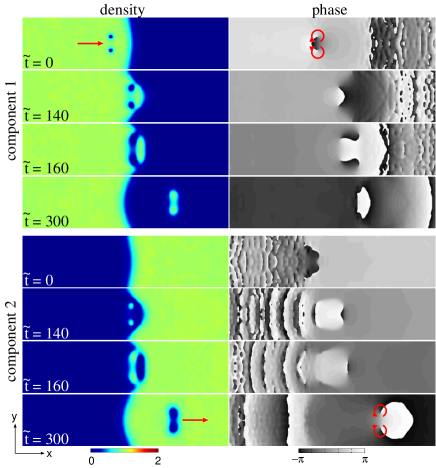
Figure 2: (Color online) Dynamics of normalized density profiles $|\psi_{j}|^{2}/n_{0}$ and phase profiles ${\rm arg}\,\psi_{j}$ for $\Delta=0.05$ and $v_{\rm in}=0.12v_{\rm s}$. The direction of the vortex dipole propagation is indicated by the arrows in the left panels, and the circulations of vortices are indicated by the arrows in the right panels. The field of view of each panel is $120\xi\times 30\xi$.

Figure 2 shows the case of a thinner interface (larger $\Delta$) and a slower vortex dipole compared with those in Fig. 1. When a vortex dipole approaches the interface, the straight interface is curved due to the forward atomic flow in front of the vortex dipole ($|\psi_{1}|^{2}/n_{0}$ at $\tilde{t}=0$ in Fig. 2). The vortex dipole then significantly deforms the interface ($|\psi_{j}|^{2}/n_{0}$ at $\tilde{t}=140$ and $\tilde{t}=160$ in Fig. 2), which creates a new vortex dipole in component 2. The vortex dipole created in component 2 then propagates in component 2, whose cores are occupied by component 1 ($\tilde{t}=300$ in Fig. 2). Generation of such a “coreless vortex dipole” by a moving potential is reported in Ref. Gautam . If the incident velocity of the vortex dipole is slightly slower, a greater fraction of component 1 is taken away from the interface, which forms an elliptic ”bubble” of component 1 moving through component 2, as in Fig. 1 of Ref. Sasaki .

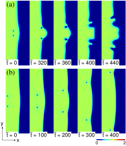
Figure 3: (Color online) Dynamics of normalized density profile $|\psi_{1}|^{2}/n_{0}$ of component 1 for (a) $\Delta=0.05$ and $v_{\rm in}=0.088v_{\rm s}$ and (b) $\Delta=0.2$ and $v_{\rm in}=0.039v_{\rm s}$. The field of view of each panel is $60\xi\times 160\xi$.

Figure 3 (a) shows the dynamics for an incident velocity $v_{\rm in}$ slower than that in Fig. 2 with the same $\Delta$. As the vortex dipole approaches the interface, the distance between the vortices increases and the interface is upheaved [$\tilde{t}=320$-$360$ in Fig. 3 (a)]. When the vortices touch the interface, the interface is disturbed and the disturbance propagates along the interface [$\tilde{t}=400$–$440$ in Fig. 3 (a)]. In these dynamics, vortices are not transferred to component 2, and the vortex penetration as in Figs. 1 and 2 does not occur.

In Fig. 3 (b), the velocity of the vortex dipole is slower and the width of the interface is thinner than for Fig. 3 (a). Near the interface, the vortex and antivortex separate and move along the interface in opposite directions. This behavior of vortices is similar to that of classical point vortices near a rigid wall. For an inviscid, incompressible, and irrotatinal fluid, the trajectories of point vortices are given by Lamb

$$\frac{1}{x^{2}}+\frac{1}{y^{2}}=\frac{4}{d^{2}},$$ (8)

where $d$ is the distance between incident vortices and the wall is located at $x=0$ or $y=0$. According to Eq. (8), the distance between the trajectories and the wall approaches $d/2$ asymptotically, which roughly agrees with the trajectories of the vortices in Fig. 3 (b).

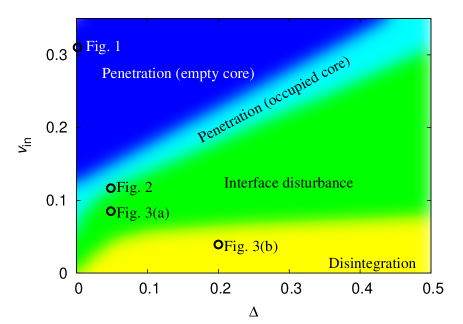
Figure 4: (Color online) Dependence of the dynamics of a vortex dipole on $\Delta$ and $v_{\rm in}$. The region of “Penetration (empty core)” corresponds to the penetration dynamics of a vortex dipole as shown in Fig. 1. In the region of “Penetration (occupied core)” the cores of a vortex dipole after the penetration are occupied by component 1, as in Fig. 2. The regions of “Interface disturbance” and “Disintegration” correspond to the dynamics shown in Figs. 3 (a) and 3 (b), respectively. The circles indicate the parameters used in Figs. 1-3.

A vortex dipole moving toward an interface thus shows a variety of dynamics as shown in Figs. 1-3, which depend on the incident velocity $v_{\rm in}$ of a vortex dipole and the parameter $\Delta$. Figure 4 shows the parameter dependence of the dynamics of a vortex dipole. The penetration of a vortex dipole across the interface occurs for large $v_{\rm in}$ and small $\Delta$. For small $v_{\rm in}$ and large $\Delta$, a vortex dipole behaves as if the interface is a rigid boundary. The region in which a vortex dipole disappears, disturbing the interface, is located between these regions.

The parameter dependence in Fig. 4 can be understood qualitatively. A vortex dipole cannot penetrate the interface, when the energy of the vortex dipole $E_{\rm vd}\simeq 2\pi\hbar^{2}n_{0}m^{-1}\log(d/\xi)$ Donnely is much smaller than the energy to deform the interface $E_{\rm interface}\sim\sigma d$, where $\sigma$ is the interfacial tension coefficient. Using the expression for the interfacial tension coefficient in Refs. Barankov ; Schae , $\sigma=gn_{0}^{2}\xi\Delta^{1/2}$, which is valid for $\Delta\lesssim 0.3$, the inequality $E_{\rm vd}\ll E_{\rm interface}$ reduces to

$$w\ll d,$$ (9)

where $w\sim\xi/\sqrt{\Delta}$ is the width of the interface and $\xi\lesssim d$ is assumed. Equation (9) indicates that the penetration of a vortex dipole is prohibited for large $\Delta$ and small $v_{\rm vd}$, which is in agreement with Fig. 4. We also expect that the penetration of a vortex dipole is prohibited when the velocity $v_{\rm cw}$ of the capillary wave on the interface is much faster than the velocity of a vortex dipole $v_{\rm vd}\simeq\hbar/(md)$, since the disturbance of the interface spreads out rapidly before the vortex dipole is transferred across the interface, as shown in Fig. 3 (a). The dispersion relation of the capillary wave, $\omega^{2}=\sigma k^{3}/(2mn_{0})$, gives $v_{\rm cw}\sim[\sigma k/(mn_{0})]^{1/2}$, and the inequality $v_{\rm cw}\gg v_{\rm vd}$ again leads to Eq. (9). In fluid mechanics, the ratio of inertial force to the surface or interfacial tension force is called the Weber number, defined by ${\rm We}=\rho v^{2}\ell/\sigma$, where $\rho$ is mass density, $v$ is characteristic velocity, and $\ell$ is characteristic length. The substitution of $\rho=mn_{0}$, $v=v_{\rm vd}$, and $\ell=d$ gives ${\rm We}\sim w/d$, and therefore the penetration of a vortex dipole is prohibited for ${\rm We}\ll 1$.

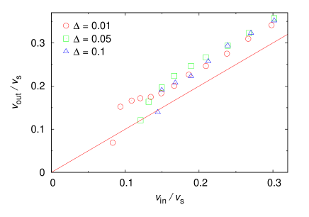
Figure 5: (Color online) Incident velocity $v_{\rm in}$ of a vortex dipole versus outgoing velocity $v_{\rm out}$ after the penetration across the interface for $\Delta=0.01$ (circles), $0.05$ (squares), and $0.1$ (triangles). The line indicates $v_{\rm in}=v_{\rm out}$.

Figure 5 shows the relation between the incident velocity $v_{\rm in}$ and outgoing velocity $v_{\rm out}$ of a vortex dipole before and after the penetration of the interface. For a sufficiently large incident velocity, the outgoing velocity exceeds the incident velocity. This is understood from the relation between the energy $E_{\rm vd}$ and velocity $v_{\rm vd}$ of a vortex dipole,

$$E_{\rm vd}\sim\frac{2\pi n_{0}\hbar^{2}}{m}\log\frac{d}{\xi}\simeq\frac{2\pi n_{0}\hbar^{2}}{m}\log\frac{\hbar}{m\xi v_{\rm vd}},$$ (10)

i.e., the velocity $v_{\rm vd}$ is larger for smaller energy $E_{\rm vd}$. When passing through the interface, a vortex dipole loses energy by disturbing the interface, and therefore the velocity increases. In Fig. 5, $v_{\rm out}$ rapidly falls to $\lesssim v_{\rm in}$ for a small $v_{\rm in}$, which corresponds to the “penetration (occupied core)” region in Fig. 4. In this parameter region, the energy is given by

$$E_{\rm vd}\sim\frac{2\pi n_{0}\hbar^{2}}{m}\log\frac{\hbar}{m\xi v_{\rm out}}+\frac{1}{2}m_{\rm core}v_{\rm out}^{2},$$ (11)

where $m_{\rm core}$ is the mass of component 1 occupying the cores of a vortex dipole after the penetration. Since $m_{\rm core}$ rapidly increases with a decrease in $v_{\rm in}$ in this parameter region, and since the $v_{\rm out}$ dependence of the right-hand side of Eq. (11) is dominated by the second term, $v_{\rm out}$ rapidly falls with a decrease in $v_{\rm in}$.

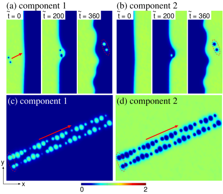
Figure 6: (Color online) (a), (b) Snapshots and (c), (d) stroboscopic images of the normalized density profiles $|\psi_{j}|^{2}$ for $\Delta=0.05$, $v=0.13v_{\rm s}$, and the incident angle, $\tan^{-1}0.4$. In (c) and (d), the images from $\tilde{t}=360$ to $\tilde{t}=1200$ are superimposed at time intervals of $\Delta\tilde{t}=40$. The images in the dashed circles in (a) and (b) correspond to those in (c) and (d), respectively. The direction of vortex dipole propagation is indicated by the arrows. The field of view of each panel is $50\xi\times 120\xi$ in (a) and (b), and $120\xi\times 80\xi$ in (c) and (d).

We also examined various incident angles and found an interesting phenomenon. Figure 6 shows the dynamics for oblique incidence of a vortex dipole. As shown in Figs. 6 (a) and 6 (b), the vortex dipole penetrates the interface in a manner similar to Fig. 2. After that, a fraction of component 1 occupying the vortex cores of component 2 oscillates between the two cores [Fig. 6 (c)]. This phenomenon is due to the tunneling of a fraction of component 1 in an effective double well potential produced by the vortex cores of component 2. If the distance between a vortex and antivortex of a vortex dipole after the penetration is larger, the tunneling rate is smaller and no oscillation is observed in the relevant time scale even when only one core is occupied by component 1 (data not shown).

IV Dynamics of vortex dipoles in a trapped system

We next study the dynamics of a two-component BEC confined in a quasi-2D axisymmetric harmonic trap $m_{j}\omega^{2}(x^{2}+y^{2})/2$. The system is tightly confined in the $z$ direction by a harmonic potential $m_{j}\omega_{z}^{2}z^{2}/2$, and the effective interaction coefficient in Eq. (3) has the form $g_{jj^{\prime}}=[\omega_{z}/(2\pi\omega)]^{1/2}G_{jj^{\prime}}$. We assume that the trap frequencies are the same for both components and that the gravitational sag is negligible. In the following simulations, we use $\omega=2\pi\times 25$ Hz and $\omega_{z}=2\pi\times 1.25$ kHz. We employ the $|F=1,m_{F}=-1\rangle$ state of ${}^{87}{\rm Rb}$ for component 1 and $|F=2,m_{F}=-2\rangle$ state of ${}^{85}{\rm Rb}$ for component 2, where $a_{11}=99a_{\rm B}$ and $a_{12}=213a_{\rm B}$ with $a_{\rm B}$ being the Bohr radius. In the experiment reported in Ref. Papp , the scattering length of ${}^{85}{\rm Rb}$ atoms, $a_{22}$, was controlled using the magnetic Feshbach resonance. We assume here that $a_{22}$ is tuned to $a_{22}=250a_{\rm B}>a_{11}$, and component 2 surrounds component 1 in the ground state. The total number of atoms is $4\times 10^{4}$ with an equal population in each component.

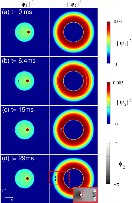
Figure 7: (Color online) Snapshots of the density profiles $|\psi_{j}|^{2}$ of the dynamics for $T=1.0$ ms. The inset magnifies the phase profile ${\rm arg}\,\psi_{2}$ in the dashed square. The arrows in the inset indicate the directions of circulation. The unit of density is $8.4\times 10^{11}$ ${\rm cm}^{-2}$. The field of view of each panel is $54.3\times 54.3$ $\mu{\rm m}$.

We create a vortex dipole by the same method Aioi as in the previous section, i.e., the attractive Gaussian potential in Eq. (7) is applied to the inner component (component 1). The Gaussian potential with intensity $V_{0}=-200\hbar\omega$ and waist $w=1.09$ $\mu{\rm m}$ is moved as

$$x_{0}(t)=\left\{\begin{array}[]{cc}X_{0}-ut&(0\leq t\leq T)\\ X_{0}-uT&(t>T),\end{array}\right.$$ (12)

with $X_{0}=4.36$ $\mu{\rm m}$, $u=1.1$ ${\rm mm}/{\rm s}$, and $y_{0}=0$. The velocity of a vortex dipole is controlled by varying $T$. We first prepare the ground state for $x_{0}=X_{0}$ by the imaginary-time propagation method [Fig. 7 (a)], and then switch to real-time propagation.

Figure 7 shows the time evolution of the system for $T=1.0$ ms, for which a vortex dipole with velocity $\simeq 1.2$ ${\rm mm}/{\rm s}$ is created and launched in the $-x$ direction [Fig. 7 (b)]. The vortex dipole then penetrates the interface [Fig. 7 (c)]. After the penetration, the cores of the vortex dipole are slightly occupied by component 1 [see the left panel of Fig. 7 (c)]. When the vortex dipole reaches the edge of the condensate [Fig. 7 (d)], the vortices disintegrate and move in the opposite directions along the circular edge (data not shown), as observed in the experiment in Ref. Neely .

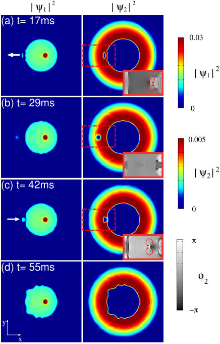
Figure 8: (Color online) Snapshots of the density profiles $|\psi_{j}|^{2}$ of the dynamics for $T=1.4$ ms. The white arrows indicate the directions of propagation. The insets magnify the phase profile ${\rm arg}\,\psi_{2}$ in the dashed squares. The arrows in the insets indicate the directions of circulation. The unit of density is $8.4\times 10^{11}$ ${\rm cm}^{-2}$. The field of view of each panel is $54.3\times 54.3$ $\mu{\rm m}$.

Figure 8 shows the case of $T=1.4$ ms, which produces a vortex dipole with velocity $\simeq 1.1$ ${\rm mm}/{\rm s}$. The vortex dipole penetrates the interface [Fig. 8 (a)], and the pair of vortices merges, in which component 1 contained in the cores also merges to become a droplet [Fig. 8 (b)]. The droplet then turns back to the center, forming a vortex–antivortex pair in component 2 [Fig. 8 (c)]. The directions of circulation of the vortex pair in Fig. 8 (c) are opposite to those in Fig. 8 (a). When the droplet reaches the inner component, it eventually disappears and the interfacial wave remains [Fig. 8 (d)].

The behaviors of the vortices in Fig. 8 can be understood as follows. The fraction of component 1 dragged into component 2 experiences a force towards the center. When the vortex dipole moves outwards [Fig. 8 (a)], it experiences a force in the direction opposite to the propagation, and the pair of vortices approach each other due to the Magnus effect (see Fig. 9 of Ref. Aioi ). When the droplet is pushed [Fig. 8 (c)], the flow around the droplet forms a vortex dipole. If the droplet propagated further without reaching the interface, it would split into two droplets (as in Fig. 2 of Ref. Sasaki ).

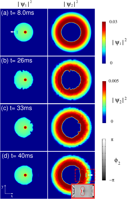
Figure 9: (Color online) Snapshots of the density profiles $|\psi_{j}|^{2}$ of the dynamics for $T=2.4$ ms. The white arrow indicates the direction of propagation. The inset magnifies the phase profile ${\rm arg}\,\psi_{2}$ in the dashed square. The arrows in the insets indicate the directions of circulation. The unit of density is $8.4\times 10^{11}$ ${\rm cm}^{-2}$. The field of view of each panel is $54.3\times 54.3$ $\mu{\rm m}$.

Figure 9 shows more complicated dynamics, where a vortex dipole with velocity $\simeq 0.9$ ${\rm mm}/{\rm s}$ is produced with $T=2.4$ ms. In this case, the penetration does not occur and the vortex dipole disappears at the interface. The interface is disturbed and the disturbance propagates along the interface [Figs. 9 (b) and 9 (c)]. Interestingly, the disturbance refocuses at the opposite side of the circular interface and a vortex dipole is created in component 2, which propagates in the $+x$ direction [Fig. 9 (d)].

V Conclusions

We have investigated the dynamics of quantized vortex dipoles in phase-separated two-component BECs. Solving the GP equation numerically, we found that a vortex dipole can penetrate an interface between the two components (say, from component 1 to component 2), in which quantized vortices in component 1 are transferred to component 2 (Figs. 1 and 2). The cores of the transmitted vortex dipole in component 2 are almost empty (Fig. 1) or occupied by component 1 (Fig. 2). When the incident velocity is slow or the width of the interface is thin, a vortex dipole cannot penetrate the interface and the vortex dipole disappears, disturbing the interface [Fig. 3 (a)], or the vortex and antivortex disintegrate and move along the interface [Fig. 3 (b)]. Through systematic numerical simulations, we obtained the parameter dependence of the dynamics (Fig. 4) and the relation between incident and outgoing velocities (Fig. 5). When a vortex dipole penetrates the interface at an oblique angle, the cores of the vortex dipole in component 2 are occupied by component 1 asymmetrically, followed by oscillation of component 1 between the cores due to tunneling.

We also found a variety of dynamics for a trapped system (Figs. 7-9). After the penetration of the interface, vortices of a vortex dipole disintegrate and move around (Fig. 7), or change to a bubble, falling back to the inner component (Fig. 8). When a vortex dipole cannot penetrate the interface, it disturbs the interface and disappears. In some cases, the disturbance of the circular interface focuses at the opposite side and reproduces a vortex dipole (Fig. 9). These predicted phenomena can be observed in, e.g., a Feshbach-controlled ${}^{85}{\rm Rb}$-${}^{87}{\rm Rb}$ BEC confined in a tight pancake-shaped trap.

- (1) S. Inouye, S. Gupta, T. Rosenband, A. P. Chikkatur, A. Görlitz, T. L. Gustavson, A. E. Leanhardt, D. E. Pritchard, and W. Ketterle, Phys. Rev. Lett. 87, 080402 (2001).
- (2) T. W. Neely, E. C. Samson, A. S. Bradley, M. J. Davis, and B. P. Anderson, Phys. Rev. Lett. 104, 160401 (2010).
- (3) D. V. Freilich, D. M. Bianchi, A. M. Kaufman, T. K. Langin, and D. S. Hall, Science 329, 1182 (2010).
- (4) S. Middelkamp, P. J. Torres, P. G. Kevrekidis, D. J. Frantzeskakis, R. Carretero-González, P. Schmelcher, D. V. Freilich, and D. S. Hall, Phys. Rev. A 84, 011605(R) (2011).
- (5) G. Roumpos, M. D. Fraser, A. Löffler, S. Höfling, A. Forchel, and Y. Yamamoto, Nature Phys. 7, 129 (2011).
- (6) G. Nardin, G. Grosso, Y. Léger, B. Piȩtka, F. Morier-Genoud, and B. Deveaud-Plédran, Nature Phys. 7, 635 (2011).
- (7) L. -C. Crasovan, V. Vekslerchik, V. M. Pérez-García, J. P. Torres, D. Mihalache, and L. Torner, Phys. Rev. A 68, 063609 (2003).
- (8) H. Lamb, Hydrodynamics, 6th ed, Sec. 155 (Dover, New York, 1945).
- (9) P. F. Linden, J. Fluid Mech. 60, 467 (1973).
- (10) W. J. M. Dahm, C. M. Scheil, and G. Tryggvason, J. Fluid Mech. 205, 1 (1989).
- (11) K. Kuehn, M. Moeller, M. Schulz, and D. Sanfelippo, Phys. Rev. E 82, 016312 (2010).
- (12) S. Gautam, P. Muruganandam, and D. Angom, arXiv:1110.2903.
- (13) W. H. Press, S. A. Teukolsky, W. T. Vetterling, B. P. Flannery, Numerical Recipes, 3rd ed, Sec. 20.7 (Cambridge Univ. Press, Cambridge, 2007).
- (14) T. Aioi, T. Kadokura, T. Kishimoto, and H. Saito, Phys. Rev. X 1, 021002 (2011).
- (15) K. Sasaki, N. Suzuki, and H. Saito, Phys. Rev. A 83, 033602 (2011).
- (16) See, e.g., R. J. Donnelly, Quantized Vortices in Helium II (Cambridge Univ. Press, Cambridge, 1991).
- (17) R. A. Barankov, Phys. Rev. A 66, 013612 (2002).
- (18) B. Van Schaeybroeck, Phys. Rev. A 78, 023624 (2008); 80, 065601 (2009).
- (19) S. B. Papp, J. M. Pino, and C. E. Wieman, Phys. Rev. Lett. 101, 040402 (2008).