Scaling metagenome sequence assembly with probabilistic de Bruijn graphs

Abstract

Deep sequencing has enabled the investigation of a wide range of environmental microbial ecosystems, but the high memory requirements for de novo assembly of short-read shotgun sequencing data from these complex populations are an increasingly large practical barrier. Here we introduce a memory-efficient graph representation with which we can analyze the k-mer connectivity of metagenomic samples. The graph representation is based on a probabilistic data structure, a Bloom filter, that allows us to efficiently store assembly graphs in as little as 4 bits per k-mer, albeit inexactly. We show that this data structure accurately represents DNA assembly graphs in low memory. We apply this data structure to the problem of partitioning assembly graphs into components as a prelude to assembly, and show that this reduces the overall memory requirements for de novo assembly of metagenomes. On one soil metagenome assembly, this approach achieves a nearly 40-fold decrease in the maximum memory requirements for assembly. This probabilistic graph representation is a significant theoretical advance in storing assembly graphs and also yields immediate leverage on metagenomic assembly.

1 Introduction

De novo assembly of shotgun sequencing reads into longer contiguous sequences plays an important role in virtually all genomic research [1]. However, current computational methods for sequence assembly do not scale well to the volume of sequencing data now readily available from next-generation sequencing machines [1, 2]. In particular, the deep sequencing required to sample complex microbial environments easily results in data sets that surpass the working memory of available computers [3, 4].

Deep sequencing and assembly of short reads is particularly important for the sequencing and analysis of complex microbial ecosystems, which can contain millions of different microbial species [5, 6]. These ecosystems mediate important biogeochemical processes but are still poorly understood at a molecular level, in large part because they consist of many microbes that cannot be cultured or studied individually in the lab [5, 7]. Ensemble sequencing (“metagenomics”) of these complex environments is one of the few ways to render them accessible, and has resulted in substantial early progress in understanding the microbial composition and function of the ocean, human gut, cow rumen, and permafrost soil [3, 4, 8, 9]. However, as sequencing capacity grows, the assembly of sequences from these complex samples has become increasingly computationally challenging. Current methods for short-read assembly rely on inexact data reduction in which reads from low-abundance organisms are discarded, biasing analyses towards high-abundance organisms [3, 4, 9].

The predominant assembly formalism applied to short-read sequencing data sets is a de Bruijn graph [10, 11, 12]. In a de Bruijn graph approach, sequencing reads are decomposed into fixed-length words, or k-mers, and used to build a connectivity graph. This graph is then traversed to determine contiguous sequences [12]. Because de Bruijn graphs store only k-mers, memory usage scales with the number of unique k-mers in the data set rather than the number of reads [13, 12]. Thus human genomes can be assembled in less than 512GB of system memory [14]. For more complex samples such as soil metagenomes, which may possess millions or more species, terabytes of memory would be required to store the graph. Moreover, the wide variation in species abundance limits the utility of standard memory-reduction practices such as abundance-based error-correction [15].

In this work, we describe a simple probabilistic representation for storing de Bruijn graphs in memory, based on Bloom filters [16]. Bloom filters are fixed-memory probabilistic data structures for storing sparse sets; essentially hash tables without collision detection, set membership queries on Bloom filters can yield false positives but not false negatives. While Bloom filters have been used in bioinformatics software tools in the past, they have not been used for storing assembly graphs[17, 18, 19, 20]. We show that this probabilistic graph representation more efficiently stores de Bruijn graphs than any possible exact representation, for a wide range of useful parameters. We also demonstrate that it can be used to store and traverse actual DNA de Bruijn graphs with a 20- to 40-fold decrease in memory usage over two common de Bruijn graph-based assemblers, Velvet and ABySS [21, 22]. We relate changes in local and global graph connectivity to the false positive rate of the underlying Bloom filters, and show that the graph’s global structure is accurate for false positive rates of 15% or lower, corresponding to a lower memory limit of approximately 4 bits per graph node.

We apply this graph representation to reduce the memory needed to assemble a soil metagenome sample, through the use of read partitioning. Partitioning separates a de Bruijn graph up into disconnected graph components; these components can be used to subdivide sequencing reads into disconnected subsets that can be assembled separately. This exploits a convenient biological feature of metagenomic samples: they contain many microbes that should not assemble together. Graph partitioning has been used to improve the quality of metagenome and transcriptome assemblies by adapting assembly parameters to local coverage of the graph [23, 24, 25]. However, to our knowledge, partitioning has not been applied to scaling metagenome assembly. By applying the probabilistic de Bruijn graph representation to the problem of partitioning, we achieve a dramatic decrease of nearly 40-fold in the memory required for assembly of a soil metagenome.

2 Results

2.1 Bloom filters can store de Bruijn graphs

Given a set of short DNA sequences, or reads, we first break down each read into a set of overlapping k-mers. We then store each k-mer in a Bloom filter, a probabilistic data structure for storing elements from sparse data sets (see Methods for implementation details). Each k-mer serves as a vertex in a graph, with an edge between two vertices $N_{1}$ and $N_{2}$ if and only if $N_{1}$ and $N_{2}$ share a (k-1)-mer that is a prefix of $N_{1}$ and a postfix of $N_{2}$, or vice versa. This edge is not stored explicitly, which can lead to false connections when two reads abut but do not overlap; these false connections manifest as false positives, discussed in detail below.

Thus each k-mer has up to 8 edges connecting to 8 neighboring k-mers, which can be determined by simply building all possible 1-base extensions and testing for their presence in the Bloom filter. In doing so, we implicitly treat the graph as a simple graph as opposed to a multigraph, which means that there can be no self-loops or parallel edges between vertices/k-mers. By relying on Bloom filters, the size of the data structure is fixed: no extra memory is used as additional data is added.

This graph structure is effectively compressible because one can choose a larger or smaller size for the underlying Bloom filters; for a fixed number of entries, a larger Bloom filter has lower occupancy and produces correspondingly fewer false positives, while a smaller Bloom filter has higher occupancy and produces more false positives. In exchange for memory, we can store k-mer nodes more or less accurately: for example, for a false positive rate of 15%, at which 1 in 6 random k-mers tested would be falsely considered present, each real k-mer can be stored in under 4 bits of memory (see Table 1). While there are many false k-mers, they only matter if they connect to a real k-mer.

The false positive rate inherent in Bloom filters thus raises one concern for graph storage: in contrast to an exact graph storage, there is a chance that a k-mer will be adjacent to a false positive k-mer. That is, a k-mer may connect to another k-mer that does not actually exist in the original dataset but nonetheless registers as present, due to the probabilistic nature of the Bloom filter. As the memory per real k-mer is decreased, false positive vertices and edges are gained, so compressing the graph results in a more tightly interconnected graph. If the false positive rate is too high, the graph structure will be dominated by false connectivity – but what rate is “too high”? We study this key question in detail below.

2.2 False positives cause local elaboration of graph structure

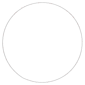
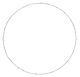
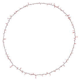
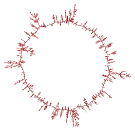
Figure 2: Graph visualizations demonstrating the decreasing fidelity of graph structure with increasing false positive rate. Erroneous k-mers are colored red and k-mers corresponding to the original generated sequence (1,000 31-mers generated by a 1,031 bp circular chromosome) are black. From top left to bottom right, the false positive rates are 0.01, 0.05, 0.10, and 0.15. Shortcuts “across” the graph are not created.

Erroneous neighbors created by false positives can alter the graph structure. To better understand this effect, we generated a random 1,031bp circular sequence and visualized the effect of different false positive rates. After storing this single sequence in compressible graphs using $k=31$ with four different false positive rates ($p_{f}$=0.01, 0.05, 0.10, and 0.15), we explored the graph using breadth-first search beginning at the first 31-mer. The graphs in Figure 2 illustrate how the false positive k-mers connected to the original k-mers (from the 1,031bp sequence) elaborate with the false positive rate while the overall circular graph structure remains, with no erroneous shortcuts between k-mers that are present in the original sequence. It is visually apparent that even a high false positive rate of 15% does not systematically and erroneously connect distant k-mers.

2.3 False long-range connectivity is a nonlinear function of the false positive rate

To explore the point at which our data structure systematically engenders false long-range connections, we inserted random k-mers into Bloom filters with increasing false positive rates. These k-mers connect to other k-mers to form graph components that increase in size with the false positive rate. We then calculated the average component size in the graph for each false positive rate ($n=10000$) and used percentile bootstrap to obtain estimates within a 95% confidence interval. Figure 3 demonstrates that the average component size rapidly increases as a specific threshold is approached, which appears to be at a false positive rate near 0.18 for k=31. Beyond 0.18, the components begin to join together into larger components.

As the false positive rate increases, we observe a sudden transition from many small components to fewer, larger components created by erroneous connections between the “true” components (Figure 3). In contrast to the linear increase in the local neighborhood structure as the false positive rate increases linearly, the change in global graph structure is abrupt as previously disconnected components join together. This rapid change resembles a geometric phase transition, which for graphs can be discussed in terms of percolation theory [26]. We can map our problem to site percolation by considering a probability $p$ that a particular k-mer is present, or “on”. (This is in contrast to bond percolation where $p$ represents the probability of a particular edge being present.) As long as the false positive rate is below the percolation threshold $p_{\theta}$ (i.e. in the subcritical phase), we would predict that the graph is not highly connected by false positives.

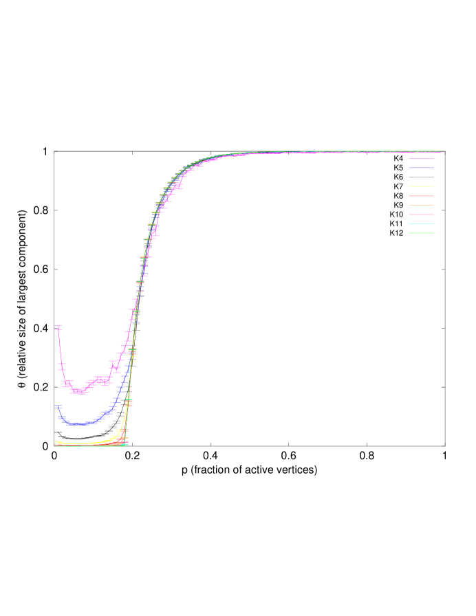
Figure S1: Demonstration of k independence by determining the percolation threshold with multiple values of k (5-12). $p$ on the x axis is the fraction of nodes present, and $\theta$ on the y axis is the fraction of nodes in the largest component. Lower values of k have greater finite size sampling errors.

Percolation thresholds for finite graphs can be estimated by finding where the component size distribution transitions from linear to quadratic in form [27]. Using the calculation method described in Methods, we found the site percolation threshold for DNA de Bruijn graphs to be $p_{\theta}=0.183\pm 0.001$ for k between 5 and 12. Although we only tested within this limited range of k, the percolation threshold appears to be independent of different $k$ (see Figure S1). Thus, as long as the false positive rate is below $0.183$, we predict that truly disconnected components in the graph are unlikely to connect to one another erroneously, that is, due to errors introduced by the probabilistic representation.

2.4 Large-scale graph structure is retained up to the percolation threshold

The results from component size analysis and the percolation threshold estimation suggest that global connectivity of the graph is unlikely to change below a false positive rate of 18%. Do we see this invariance in global connectivity in other graph measures?

To assess global connectivity, we employed the diameter metric in graph theory, the length of the “longest shortest” path between any two vertices [28]. If shorter paths between real k-mers were being systematically generated due to false positives, we would expect the diameter of components to decrease as the false positive rate increased. We randomly generated 58bp long circular chromosomes (50bp read with the first 8-mer appended to the end of the string) to construct components containing 50 8-mers and calculated the diameter at different false positive rates. We kept $k$ low because we needed to be able to exhaustively explore the graph even beyond the percolation threshold, which is computationally prohibitive to do at higher k values. Furthermore, larger circular chromosomes would be more likely to erroneously connect at a fixed $k$, but due to the relatively low number of possible 8-mers, we had to keep the chromosomes small. We only considered paths between two real k-mers in the dataset.

At each false positive rate, we ran the simulation 500 times and estimated the mean within a 95% confidence interval using percentile bootstrap. As Figure 4 shows, erroneous connections between pairs of real k-mers are rare below a false positive rate of 20%. For false positive rates above this threshold, spurious connections between real k-mers are created, which lowers the diameter. Thus, the larger scale graph structure is retained up through $p=0.183$, as suggested by the component size analysis and percolation results. This demonstrates that as long as the k-mer space is only sparsely occupied by false positives, long “bridges” between distant k-mers do not appear spontaneously.

2.5 Erroneous k-mers from sequencing eclipse graph false positives

It is important to compare the errors from false positives in the de Bruijn graph representation with errors from real data. In particular, real data from massively parallel sequencers will contain base calling errors. In de Bruijn graph-based assemblers, these sequencing errors add to the graph complexity and make it more difficult to find high-quality paths for generating long, accurate contigs. Since our approach also generates false positives, we wanted to compare the error rate from the Bloom filter graph with experimental errors generated by sequencing (Table 2). We used the E. coli K-12 MG1665 genome to compare various graph invariants between an Illumina dataset generated from the same strain (see Methods), an exact representation of the genome, and inexact representations with different false positive rates.

For these comparisons, we used a $k$ value of 17, for which we can store graphs exactly, i.e. we have no false positives because we can store $4^{17}$ entries precisely in 2GB of system memory. This is equivalent to a Bloom filter with one hash table and a 0% false positive rate. We found a total of 50,605 17-mers in the exact representation that were not part of a simple line, i.e. had more than two neighbors (degree $>$ 2). As the false positive rate increased, the number of these 17-mers increased in the expected linear fashion. Furthermore, the number of real 17-mers, those that are not false positives, comprise the majority of the graph. (As above, we only counted false positive k-mers that are transitively connected to at least one real k-mer.)

In contrast, when we examined an exact representation of an Illumina dataset, only 9.9% of the k-mers in the graph truly exist in the reference genome. The number of 17-mers with more than 2 neighbors in the sequencing reads is higher than for the exact representation of the genome, which demonstrates that sequencing errors add to the complexity of the graph. Overall, the errors demonstrated by sequencers dwarf the errors caused by the inexact graph representation at a reasonable false positive rate.

When we assemble this data set with the Velvet and ABySS assemblers at k=31, Velvet requires 3.7GB to assemble the data set, while ABySS requires 1.6GB; this memory usage is dominated by the graph storage [29]. Thus the Bloom filter approach stores graphs 30 or more times more efficiently than either program, even with a low false positive rate of 1%. While this direct comparison can not be made fairly – assemblers store the graph as well as k-mer abundances and other information – it does suggest that there are opportunities for decreasing memory usage with the probabilistic graph representation.

2.6 Sequences can be accurately partitioned by graph connectivity

Can we use this low-memory graph representation to find and separate components in de Bruijn graphs? The primary concern is that false positive nodes or edges would connect components, but the diameter results suggest that components are unlikely to connect below a 20% false positive rate. To verify this, we analyzed a simulated dataset of 1,000 randomly generated sequences of length 10,000 bp. Using $k=31$, we partitioned the data across many different false positive rates, using the procedure described in Methods. As predicted, the resulting number of partitions did not vary across the false positive rates while $f_{p}\leq 0.15$ (Figure S2).

We then applied partitioning to a considerably larger bulk soil metagenome (“MSB2”) containing 35 million 75 bp long reads generated from an Illumina GAII sequencer. We calculated the number of unique 31-mers present in the data set to be 1.35 billion. Then, for each of several false positive rates (see Table 3) we loaded the reads into a graph, eliminated components containing fewer than 200 unique k-mers, and partitioned the reads into separate files based on graph connectivity.

Once we obtained the partition sets, we individually assembled each set of partitions using ABySS, as well as the entire (unpartitioned) data set, retaining contigs longer than 500 bp. The resulting assemblies were all identical, containing 1,444 contigs with a total assembled sequence of 1.07 megabases. The unpartitioned data set required 33GB to assemble with ABySS, while the data set could be partitioned in under 1 GB with a 30-fold decrease in maximum memory usage (Table 3). Moreover, despite this dramatic decrease in the memory required to assemble the data set, the assembly results are identical.

3 Discussion

3.1 Bloom filters can be used to efficiently store de Bruijn graphs

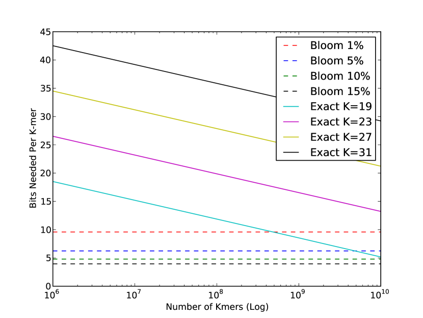
Figure 5: Comparison between Bloom filters at different false positive rates with the information-theoretic lossless lower bound at different k values. Bloom filters are k independent and are more efficient than any lossless data structure for higher k due to greater sparseness in k-mers inserted compared to all possible k-mers.

The use of Bloom filters to store a de Bruijn graph is straightforward and memory efficient. The expected false positive rate can be tuned based on desired memory usage, yielding a wide range of possible storage efficiencies (Table 1). Since memory usage is k independent in Bloom filters, it is more efficient than the theoretical lower-bound for a lossless exact representation when the number of k-mers inserted in the graph is sparsely populated, which is dependent on k (Figure 5; see [13] for details on lower-bound memory usage for an exact representation).

Even for low false positive rates such as 1%, this is still an efficient graph representation, with significant improvements in both theoretical memory usage (Figure 5) and actual memory usage compared to two existing assemblers, Velvet and ABySS (Table 2). We can store k-mers in this data structure with a much smaller set of “erroneous” k-mers than those generated by sequencing errors, and the Bloom filter false positive rates have less of an effect on branching graph structure than do sequencing errors. In addition, the false positives engendered by the Bloom filters are uncorrelated with the original sequence, unlike single-base sequencing errors which resemble the real sequence.

Using a probabilistic graph representation with false positive nodes and edges raises the specter of systematic graph artifacts resulting from the false positives. For partitioning, our primary concern was that false positives would incorrectly connect components, rendering partitioning ineffective. The results from percolation analysis, diameter calculations, and partitioning of simulated and real data demonstrate that below the calculated percolation threshold there is no significant false connectivity. As long as the false positive rate is below 18.3%, long false paths are not spontaneously created and the large scale graph properties do not change. Above this rate, the global graph structure slowly degrades.

3.2 Partitioning works on real data sets

Our partitioning results on a real soil metagenome, the MSB2 data set, demonstrate the utility of partitioning for reducing memory usage. For this specific data set, we obtained identical results with a 20-40x decrease in memory (Table 3). This is consonant with our results from storing the E. coli genome, in which we achieved a 30-fold decrease in memory usage over the exact representation at a false positive rate of 1%. While increased coverage and variation in data set complexity will affect actual memory usage for other data sets, these results demonstrate that significant scaling in the memory required for assembly can be achieved in one real case.

The memory requirements for the partitioning process on the MSB2 data set are dominated by the memory required to store and explore the graph; the higher memory usage observed for partitioning at a false positive rate of 15% is due to the increase in component size from local false positives. Regardless, the memory requirements for downstream assembly of partitions is driven by the size of the largest partition, which here is very small (345,000 reads; Table 3) due to the high diversity of soil and the concordant low coverage. The dominant partition size is remarkably refractory to the graph’s false positive rate, increasing by far less than 1% for a 15-fold increase in false positives; this shows that our theoretical and simulated results for component size and diameter apply to the MSB2 data set as well.

Once partitioned, components can be assembled with parameters chosen for the coverage and sequence heterogeneity present in each partition. Moreover, data sets partitioned at a low $k_{0}$ can be exactly assembled with any $k\geq k_{0}$, because overlaps of $k_{0}-1$ bases include all overlaps of greater length. Because the partitions will generally be much smaller than the total data set (see Table 3), they can be quickly assembled with many different parameters. This ability to quickly explore many parameters could result in significant improvement in exploratory metagenome assembly, where the “best” assembly parameters are not known and must be determined empirically based on many different assemblies.

Combined with the scaling properties of the graph representation, partitioning with this probabilistic de Bruijn graph representation offers a way to efficiently apply a partitioning strategy to certain assembly problems. While this work focuses on theoretical properties of the graph representation and analyzes only one real data set, the results are promising; the next step is to evaluate the approach on many more real data sets.

3.3 Concluding thoughts

Developing efficient and accurate approaches to de novo assembly continues to be one of the “grand challenges” of bioinformatics [2]. Improved metagenome assembly approaches are particularly important for the investigation of microbial life on Earth, much of which has not been sampled [30, 7]. While our appreciation for the role that microbes play in biogeochemical processes is only growing, we are increasingly limited by our ability to analyze the data. For example, the Earth Microbiome Project is generating petabytes of sequencing data from complex microbial communities, many of which contain entirely novel ensembles of microbes; scaling de novo assembly is a critical requirement of this investigation [31].

The probabilistic de Bruijn graph representation presented here has a number of convenient features for storing and analyzing large assembly graphs. First, it is efficient and compressible: for a given data set, a wide range of false positive rates can be chosen without impacting the global structure of the graph, allowing graph storage in as little as 4 bits per k-mer. Because a higher false positive rate yields a more elaborate local structure, memory can be traded for traversal time in e.g. partitioning. Second, it is a fixed-memory data structure, with predictable degradation of both local and global structure as more data is inserted. For data sets where the number of unique k-mers is not known in advance, the occupancy of the Bloom filter can be monitored as data is inserted and directly converted to an expected false positive rate. Third, the memory usage is independent of the k-mer size chosen, making this representation convenient for exploring properties at many different parameters. It also allows the storage and traversal of de Bruijn graphs at multiple k-mer sizes within a single structure, although we have not yet explored these properties. And fourth, it supports memory-efficient partitioning, an approach that exploits underlying biological features of the data to divide the data set into disconnected subsets.

Our initial motivation for developing this use of Bloom filters was to explore partitioning as an approach to scaling metagenome assembly, but there are many additional uses beyond metagenomics. Here we describe exact partitioning of the graph into components, but inexact partitioning has been successfully applied to mRNAseq assembly [25]. Inexact partitioning, as done by the Chrysalis component of the Trinity pipeline, uses heuristics to subdivide the graph for later assembly; the data structure described in this work can be used for this purpose as well. More broadly, a more memory efficient de Bruijn graph representation opens up many additional opportunities. While de Bruijn graph approaches are currently being used primarily for the purposes of assembly, they are a generally useful formalism for sequence analysis. In particular, they have been extended to efficient multiple-sequence alignment, repeat discovery, and detection of local and structural sequence variation [29, 32, 33, 34].

We are further exploring the use of probabilistic de Bruijn graphs for graph-based error correction, graph-based homology search, and graph-based artifact detection in large sequencing data sets. The approach used in partitioning, in which we use properties measured in the de Bruijn graph to select and extract individual reads based on e.g. local graph connectivity or sequence identiy, may generalize to a variety of problems.

4 Genome and Sequence Data

We used the E. coli K-12 MG1655 genome (GenBank: U00096.2) and two MG1655 Illumina datasets (Short Read Archive accessions SRX000429 and SRX000430) for E. coli analyses. The MSB2 soil data set is available as SRA accession SRA050710.1.

5 Data Structure Implementation

We implemented a variation on the Bloom filter data structure to store k-mers in memory. In a classic Bloom filter, multiple hash functions map bits into a single hash table to add an object or test for the presence of an object in the set. In our variant, we use multiple prime-number-sized hash tables, each with a different hash function corresponding to the modulus of the DNA bitstring representation with the hash table size; this is a computationally convenient way to construct hash functions for DNA strings. The properties of this implementation are identical to a classical Bloom filter [35].

6 Estimating False Positive Rate For Erroneous Connectivity

We ran a simulation to find when components in the graph begin to erroneously connect to one another. To calculate the false positive rate $p$ at which this aberrant connectivity occurs, we added random k-mers, sampled from a uniform GC distribution, to the data structure and then calculated the occupancy and size of the largest component. From this we sampled the relative size of the largest component and the overall component size distribution for each given occupancy rate. At the occupancy where a “giant component” appears, this component size distribution should be scale-free [27]. We then found at what value of $p$ the resulting component size distribution in logarithmic scale can be better fitted in a linear or quadratic fashion using the F-statistic

$$F=\frac{RSS_{1}-RSS_{2}}{p_{2}-p_{1}}\times\frac{n-p_{2}}{RSS_{2}}$$

where $RSS_{i}$ is the residual sum of squares for model $i$, $p_{i}$ is the number of parameters for model $i$, and $n$ is the number of data points. To handle the finite size sampling error, the data was binned using the threshold binning method [36]. The critical value for when aberrant connectivity occurred was found by determining the local maxima of the F-values [37].

7 Graph Partitioning Using A Bloom Filter

We used the Bloom filter data structure containing the k-mers from a dataset to discover components of the graph, i.e. to partition the graph. Here a component is a set of k-mers whose originating reads overlap transitively by at least $k-1$ base pairs. Reads belonging only to small components can be discovered and eliminated in fixed memory using a simple traversal algorithm that truncates after discovering more than a given number of novel k-mers. For discovering large components we tag the graph at a minimum density by using the underlying reads as a guide. We then exhaustively explore the graph around these tags in order to connect tagged k-mers based on graph connectivity. The underlying reads in each component can then be separated based on their partition.

8 Assembler software

We used ABySS v1.3.1 and Velvet v1.1.07 to perform assemblies. The ABySS command was: mpirun -np 8 ABYSS-P -k31 -o contigs.fa reads.fa. The Velvet commands were: velveth assem 31 -fasta -short reads.fa && velvetg assem. We did not use Velvet for the partitioning analysis because Velvet’s error correction algorithm is stochastic and results in dissimilar assemblies for different read order.

9 Software and Software Availability

We have implemented this compressible graph representation and the associated partitioning algorithm in a software package named khmer. It is written in C++ and Python 2.6 and is available under the BSD open source license at https://github.com/ged-lab/khmer. The graphviz software package was used for graph visualizations. The scripts to generate the figures of this paper are available in the khmer repository.

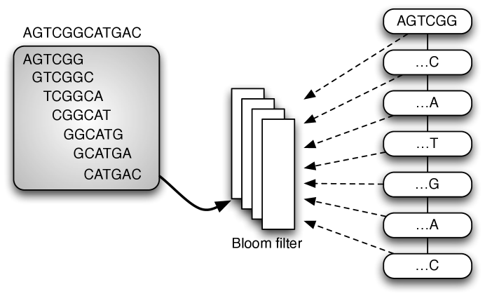
Figure 1: Storing de Bruijn graphs in Bloom filters. Longer sequences (top left) are broken down into k-mers (bottom left; here, k=6) and stored in the Bloom filter (middle). The graph (right) is traversed by starting at a k-mer and then testing all possible 1-base pre- and post-fixes for presence in the Bloom filter.

Figure 3: Average component size versus false positive rate. The average component size sharply increases as the false positive rate approaches the percolation threshold.

Figure 4: The diameter of randomly generated 58bp long circular chromosomes in 8-mer (i.e. a cycle of 50 8-mers) space remains constant for false positive rates up through 18.3%. Only real (non-error) k-mers are considered for starting and ending points.

Table 1: Bits per k-mer for various false positive rates.

False positive rate	Bits/k-mer
0.1 %	14.35
1 %	9.54
5 %	6.22
10 %	4.78
15 %	3.94
20 %	3.34

Table 2: Effects of loading E. coli data at different false positive rates

Graph	Total k-mers	False connected k-mers	% Real	Deg $>2$	Mem (bytes)
E. coli at 0%	4,530,123	0	100	50,605	$2.1\times 10^{9}$
E. coli at 1%	4,814,050	283,927	94.1	313,844	$5.4\times 10^{6}$
E. coli at 5%	6,349,301	1,819,178	71.3	1,339,102	$3.5\times 10^{6}$
E. coli at 15%	31,109,523	26,579,400	14.6	10,522,482	$2.2\times 10^{6}$
Reads at 0%	45,566,033	41,036,029	9.9	7,699,309	$2.1\times 10^{9}$
Reads at 1%	48,182,271	43,652,265	9.4	31,600,208	$5.4\times 10^{7}$
Reads at 5%	62,019,545	57,489,537	7.3	42,642,203	$3.6\times 10^{7}$
Reads at 15%	231,687,063	227,157,037	1.9	113,489,902	$2.3\times 10^{7}$

Table 3: Partitioning results on a soil metagenome at k=31.

False positive rate	Total memory use (improvement)	Largest partition size in reads
1%	1.75GB (18.8x)	344,426
5%	1.20GB (27.5x)	344,426
10%	0.96GB (34.37x)	344,426
15%	0.83GB (39.75x)	344,426

Figure S2: The graph shows the number of partitions for a simulated dataset with 1,000 contigs of 10,000 bp each (circles). For $n=5$ different combinations of hash table sizes, there was no variation in results for the simulated dataset.