Approximate homotopy series solutions of perturbed PDEs via approximate symmetry method

Abstract: We show that the two couple equations derived by approximate symmetry method and approximate homotopy symmetry method are connected by a transformation for the perturbed PDEs. Consequently, approximate homotopy series solutions can be obtained by acting the transformation on the known solutions by approximate symmetry method. Applications to the Cahn-Hilliard equation illustrate the effectiveness of the transformation.

Keywords: Approximate symmetry, Approximate homotopy symmetry, Transformation, Perturbed PDEs

1 Introduction

Group theoretical methods based on local and nonlocal symmetries provide remarkable techniques to analyze partial differential equations (PDEs) such as constructing group invariant solutions, studying integrability etc., and also build a ladder to explore profound understandings of the physics of the underlying problems such as detecting conservation laws [1, 2]. The prerequisite of achieving these goals is that the PDEs under study possess affluent symmetries, nevertheless, for the perturbed PDEs (containing a small perturbed parameter), the classical symmetry method losses its superiorities because the small parameter disturbs the symmetry group properties of the unperturbed equation, even makes the studied PDEs hold few symmetries.

In view of the drawbacks of classical symmetry method for conducting this type of equations, the integration of perturbation analysis and symmetry group theory makes two well-known approximate symmetry methods (ASM) emerge [4, 3]. The originators of the two approaches are Baikov et.al. [3] and Fushchich and Shtelen [4] who employ the standard perturbation techniques on the infinitesimal operators and dependent variables respectively. The comparisons of the two ASM which are illustrated by several specific equations may be found in [5, 6]. Quite recently, the extended combination of homotopy conception with perturbation technique and symmetry method produces approximate homotopy symmetry method (AHSM), which is suitable for studying the problems which don’t contain small parameters [7].

The distinct merit of AHSM is that the accuracy of approximate homotopy series solutions can be controlled by adjusting the convergence-control parameter, however, it is at the expense of the greater computation than ASM [8]. On the other hand, we find that the frameworks of ASM and AHSM for the perturbed PDEs are quite similar except for the different studied objects (see subsection 2.1 below). Hence, a natural question occurs: what is the relationship between ASM and AHSM, does there exist a transformation or others to link them? In [8], the authors study this problem which is exemplified by a class of perturbed nonlinear wave equations and show that first-order coupled equations and higher-order similarity reduced equations are connected by two scaling transformations respectively. However, the general results for the connections between ASM and AHSM for general perturbed PDEs are still open.

The purpose of our paper is to give a positive answer about this question. We show that the two couple equations obtained by ASM and AHSM are equivalent under a transformation. Based on this transformation, one can construct approximate homotopy series solutions directly from the known approximate solutions by ASM without performing AHSM for the governing equations.

The outline of the paper is as follows: In section 2, we briefly review some basic notions and give the main results. Section 3 concentrate on the applications of the results to the Cahn-Hilliard equation. The last section contains conclusion and discussion of our results.

2 Basic notions and principles

In this section, we first briefly review the main ideas of ASM and AHSM, and then give the results about the relationship between the two approaches.

2.1 Basic notions

We take the following $k$th-order perturbed nonlinear PDE

$$E=E_{0}(x,u,u^{(1)},\dots,u^{(k)})+\epsilon\,E_{1}(x,u,u^{(1)},\dots,u^{(k)})=0$$ (1)

into account to illustrate the main ideas of ASM and AHSM, throughout the section, with independent variables $x=(x_{1},\dots,x_{n})(n\geq 2)$, a single dependent variable $u$, $u^{(j)}=\partial^{j}u/\partial x_{1}^{j_{1}}\dots\partial x_{n}^{j_{n}}$ with $j_{1}+\dots+j_{n}=j~{}(j,j_{1},\dots,j_{n}=1,\dots,k)$ is a collection of all $j$th-order partial derivatives, $\epsilon$ is a small perturbed parameter. Note that we only use one variable $u$ to keep the notation simple, the generalization to systems being fairly obvious. Also $E_{i}=E_{i}(x,u,u^{(1)},\dots,u^{(k)})(i=0,1)$ if no special notes are added.

Let’s first recall the definition of classical symmetry. Consider the infinitesimal generator

$$X=\sum_{i=1}^{n}\xi^{i}(x,u_{0},u_{1}\dots,u^{(k)})\partial_{x_{i}}+\eta(x,u_{0},u_{1}\dots,u^{(k)})\partial_{u},$$ (2)

where $\xi^{i}$ and $\eta$ are smooth functions of their arguments. Let $X^{(k)}$ be the $k$th-prolongation of the generator $X$ calculated by the well-known prolongation formulae [1, 2].

Definition 1. (Symmetry or exact symmetry [1, 2]) The Lie symmetry $X$ of the form (2) is admitted by Eq.(1) if and only if

$$X^{(k)}E|_{E=0}=0,$$

where the notation $|_{E=0}$ means evaluated on the solution manifold of $E=0$.

The ASM originated by Fushchich and Shtelen employs a perturbation of dependent variable and then approximate symmetry of original equation is defined to the exact symmetry of the system corresponding to each order in the small parameter.

Specifically, expanding the dependent variable with respect to the small parameter $\epsilon$ yields

$$u=\sum^{\infty}_{l=0}\epsilon^{l}u_{l},$$

where $u_{l}=u_{l}(x)\,(l=0,1,2,\dots)$ stand for unknown functions throughout the paper, then substituting it into Eq.(1) and vanishing the coefficients of all different powers of $\epsilon$, one obtains a coupled system

$$\epsilon^{0}:~{}~{}E_{0}|_{\epsilon=0}=0,$$

$$\epsilon^{i}:~{}~{}\Big{[}\frac{\partial^{i}E_{0}}{\partial\epsilon^{i}}+i\,\frac{\partial^{i-1}E_{1}}{\partial\epsilon^{i-1}}\Big{]}_{|_{\epsilon=0}}=0,\quad i=1,2,\dots.$$ (3)

Definition 2. (Approximate symmetry [4]) The $i$th order approximate symmetry of Eq.(1) is defined to the exact symmetry of the first $i+1$ equations in Eq.(2.1).

For approximate homotopy symmetry of Eq.(1), one generally consider the following simple homotopy model

$$H(u,q)=(1-\theta q)E_{0}+q\epsilon(1-\theta)E_{1}=0,$$ (4)

where, hereinafter, $q\in[0,1]$ is an embedding homotopy parameter and $\theta$ denotes the convergence-control parameter. The above homotopy model has the property $H(u,0)=E_{0},\,H(u,1)=E$.

Assuming Eq.(1) has the homotopy series solutions in the form

$$u=\sum^{\infty}_{l=0}q^{l}u_{l},$$ (5)

where $u_{l}$ solve

$$q^{0}:~{}~{}E_{0}|_{q=0}=0,$$

$$q^{i}:~{}~{}\Big{[}\frac{\partial^{i}E_{0}}{\partial q^{i}}-i\theta\frac{\partial^{i-1}E_{0}}{\partial q^{i-1}}+i\epsilon(1-\theta)\frac{\partial^{i-1}E_{1}}{\partial q^{i-1}}\Big{]}_{|_{q=0}}=0,~{}~{}~{}i=1,2,\dots.$$ (6)

Equivalently, we rearrange Eq.(2.1) by eliminating $\partial^{i-1}E_{0}/\partial q^{i-1}$ in the $(i+1)$th equation by means of the first $i$ equations and transform it into the following form

$$q^{0}:~{}~{}E_{0}|_{q=0}=0,$$

$$q^{i}:~{}~{}\Big{[}\frac{\partial^{i}E_{0}}{\partial q^{i}}+\epsilon(1-\theta)\sum_{k=0}^{i-1}\theta^{i-1-k}\frac{i!}{k!}\frac{\partial^{k}E_{1}}{\partial q^{k}}\Big{]}_{|_{q=0}}=0,~{}~{}~{}i=1,2,\dots.$$ (7)

Definition 3. (Approximate homotopy symmetry [7]) The $i$th order approximate homotopy symmetry of Eq.(1) associated with homotopy model (4) corresponds to the exact symmetry of the first $i+1$ equations in Eq.(2.1) or Eq.(2.1).

Obviously, the first equation of Eq.(2.1) is the same as the first one of Eq.(2.1). When $\theta=0$, Eq.(2.1) is equivalent to Eq.(2.1) under the scaling transformation $u_{i}=\epsilon^{i}\widetilde{u}_{i}~{}(i=0,1,2,\dots)$ owing to $(\partial^{i}E_{0}/\partial q^{i})_{|_{q=0}}$ is linear about $u_{i}$ and its derivatives $u_{i}^{(\lambda)}$ (see Lemma 1 below). However, the parameter $\theta$ is used to adjust the convergence of homotopy series solution and may not be zero, thus it is the intention below to search for the connections under the condition $\theta\neq 0$.

2.2 Main results

In what follows, we first prove two basic lemmas and then establish the connections between Eq.(2.1) and Eq.(2.1).

Lemma 1. $(\partial^{n}E_{0}/\partial q^{n})_{|_{q=0}}$ is linear about $u_{n}$ and its derivatives $u_{n}^{(\lambda)}$, where $n(\geq 1)$ are positive integers and $\lambda=0,1,\dots,k$.

Proof: We take $u^{(0)}(=u),u^{(1)},\dots,u^{(k)}$ of $E_{0}$ as independent arguments and expand $u$ as (5), then by means of the generalized Faa di bruno’s formula [11], $n$th-order derivative of $E_{0}$ with respect to $q$ is

$$\frac{\partial^{n}E_{0}}{\partial q^{n}}=\sum_{0}\sum_{1}\dots\sum_{n}\frac{n!}{\prod\limits_{i=1}^{n}(i!)^{r_{i}}\prod\limits_{i=1}^{n}\prod\limits_{j=1}^{k+1}p_{ij}!}\times\frac{\partial^{r}E_{0}}{\partial[u^{(0)}]^{p_{1}}\partial[u^{(1)}]^{p_{2}}\dots\partial[u^{(k)}]^{p_{k+1}}}$$

$$\hskip 45.52458pt\times\prod_{i=1}^{n}\left(\frac{\partial^{i}u^{(0)}}{\partial q^{i}}\right)^{p_{i1}}\left(\frac{\partial^{i}u^{(1)}}{\partial q^{i}}\right)^{p_{i2}}\dots\left(\frac{\partial^{i}u^{(k)}}{\partial q^{i}}\right)^{p_{i(k+1)}},$$ (8)

where the respective sums are over all nonnegative integer solutions of the Diophantine equations, as follows

$$\sum_{0}:~{}r_{1}+2r_{2}+\dots+n\,r_{n}=n,$$

$$\sum_{m}:~{}p_{m1}+p_{m2}+\dots+p_{m(k+1)}=r_{m},~{}~{}~{}~{}m=1,2,\dots,n,$$

$$r=p_{1}+p_{2}+\dots+p_{k+1}=r_{1}+r_{2}+\dots+r_{n},$$

$$p_{j}=p_{1j}+p_{2j}+\dots+p_{nj},~{}~{}~{}~{}j=1,2,\dots,k+1,$$ (9)

and

$$\frac{\partial^{i}u^{(\lambda)}}{\partial q^{i}}=\sum^{\infty}_{l=i}\frac{l!}{(l-i)!}~{}q^{l-i}u_{l}^{(\lambda)},~{}~{}~{}\lambda=0,1,\dots,k.$$ (10)

Obviously, when $q=0$, all terms in Eq.(10) vanish except for $u_{i}^{(\lambda)}$. Similarly, Eq.(2.2) with $q=0$ becomes

$$\frac{\partial^{n}E_{0}}{\partial q^{n}}_{|_{q=0}}=\sum_{0}\sum_{1}\dots\sum_{n}\frac{n!}{\prod\limits_{i=1}^{n}\prod\limits_{j=1}^{k+1}p_{ij}!}\times\left[\frac{\partial^{r}E_{0}}{\partial[u^{(0)}]^{p_{1}}\partial[u^{(1)}]^{p_{2}}\dots\partial[u^{(k)}]^{p_{k+1}}}\right]_{|_{q=0}}$$

$$\hskip 62.59596pt\times\prod_{i=1}^{n}\left[u_{i}^{(0)}\right]^{p_{i1}}\left[u_{i}^{(1)}\right]^{p_{i2}}\dots\left[u_{i}^{(k)}\right]^{p_{i(k+1)}}.$$ (11)

In Eq.(2.2), only when $i=n$, the terms containing $u_{n}$(or its derivatives) occur. At the moment, the solution of the first equation in Eq.(2.2) $r_{n}=1,r_{i}=0(i\neq n)$ generates the terms uniquely, then other equations give $r=1$ and $p_{i}=1,p_{s}=0(s\neq i)$ and $p_{ni}=1,p_{ns}=0(s\neq i)$. Hence, the arguments $u_{n}$ and its derivatives only occur in the following terms in Eq.(2.2)

$$\frac{\partial E_{0}}{\partial u^{(0)}}_{|_{q=0}}u^{(0)}_{n},~{}~{}\frac{\partial E_{0}}{\partial u^{(1)}}_{|_{q=0}}u^{(1)}_{n},~{}~{}\dots,~{}~{}\frac{\partial E_{0}}{\partial u^{(k)}}_{|_{q=0}}u^{(k)}_{n},$$

which are linear about $u_{n}$ and its derivatives since $(\partial E_{0}/\partial u^{(i)})_{|_{q=0}}\,(i=0,1,\dots,k)$ are only functions of $x,u_{0}$ and their derivatives. Meanwhile, all other terms with $q=0$ are only functions of $x,u,u_{1},\dots,u_{n-1}$ and their derivatives, thus Lemma 1 follows. The proof ends.$~{}~{}~{}~{}\square$

Lemma 2. Substituting the transformation

$$u_{0}^{(\lambda)}=\widehat{u}_{0}^{(\lambda)},~{}~{}~{}~{}u_{l}^{(\lambda)}=\sum^{l-1}_{j=0}{l-1\choose j}\theta^{j}\widehat{u}^{(\lambda)}_{l-j},~{}~{}l=1,2,\dots,~{}\lambda=0,1,\dots,k,$$ (12)

into $(\partial^{n}E_{0}/\partial q^{n})_{|_{q=0}}$, after deleting the symbol $\,\widehat{}\,$, $[\partial^{n}E_{0}(\theta:u,\dots,u^{(k)})/\partial q^{n}]_{|_{q=0}}$ is equal to

$$\Big{[}\frac{\partial^{n}E_{0}}{\partial q^{n}}+\sum\limits_{i=2}^{n}\frac{n!}{(i-1)!}{n-1\choose i-2}\theta^{n-i+1}\frac{\partial^{i-1}E_{0}}{\partial q^{i-1}}\Big{]}_{|_{q=0}},$$ (13)

where $[\partial^{n}E_{0}(\theta:u,\dots,u^{(k)})/\partial q^{n}]_{|_{q=0}}$ denotes the transformed expression via (12) and
$(\partial^{i}E_{0}/\partial q^{i})_{|_{q=0}}(i=2,3,\dots,n)$ stand for the untransformed ones.

Proof: The main idea of the proof is to regard $[\partial^{n}E_{0}(\theta:u,\dots,u^{(k)})/\partial q^{n}]_{|_{q=0}}$ as a polynomial of $\theta$ and search for the coefficients of different degree of $\theta$ in it.

Specifically, transformation (12) makes Eq.(2.2) become

$$\frac{\partial^{n}E_{0}}{\partial q^{n}}_{|_{q=0}}=\sum_{0}\sum_{1}\dots\sum_{n}\frac{n!}{\prod\limits_{i=1}^{n}\prod\limits_{j=1}^{k+1}p_{ij}!}\times\left[\frac{\partial^{r}E_{0}}{\partial[u^{(0)}]^{p_{1}}\partial[u^{(1)}]^{p_{2}}\dots\partial[u^{(k)}]^{p_{k+1}}}\right]_{|_{q=0}}$$

$$\hskip 62.59596pt\times\prod_{i=1}^{n}\left[\sum^{i-1}_{j=0}{i-1\choose j}\theta^{j}\widehat{u}^{(0)}_{i-j}\right]^{p_{i1}}\dots\left[\sum^{i-1}_{j=0}{i-1\choose j}\theta^{j}\widehat{u}^{(k)}_{i-j}\right]^{p_{i(k+1)}}$$

$$\hskip 48.36958pt=\sum_{0}\sum_{1}\dots\sum_{n}\frac{n!}{\prod\limits_{i=1}^{n}\prod\limits_{j=1}^{k+1}p_{ij}!}\times\left[\frac{\partial^{r}E_{0}}{\partial[u^{(0)}]^{p_{1}}\partial[u^{(1)}]^{p_{2}}\dots\partial[u^{(k)}]^{p_{k+1}}}\right]_{|_{q=0}}$$

$$\hskip 62.59596pt\times[\widehat{u}^{(0)}_{1}]^{p_{11}}\dots[\widehat{u}^{(k)}_{1}]^{p_{1(k+1)}}[\widehat{u}^{(0)}_{2}+\theta\widehat{u}^{(0)}_{1}]^{p_{21}}\dots[\widehat{u}^{(k)}_{2}+\theta\widehat{u}^{(k)}_{1}]^{p_{2(k+1)}}\times\dots$$

$$\hskip 62.59596pt\times[\widehat{u}^{(0)}_{n}+\dots+\theta^{n-1}\widehat{u}^{(0)}_{1}]^{p_{n1}}\dots[\widehat{u}^{(k)}_{n}+\dots+\theta^{n-1}\widehat{u}^{(k)}_{1}]^{p_{n(k+1)}}.$$ (14)

In particular,

$$\left[\sum^{i-1}_{j=0}{i-1\choose j}\theta^{j}\widehat{u}^{(\lambda)}_{i-j}\right]^{p_{i\nu}}=\sum\frac{p_{i\nu}!\left[\widehat{u}_{i}^{(\lambda)}\right]^{a_{\nu 0}}}{a_{\nu 0}!\dots a_{\nu(i-1)}!}\left[(i-1)\theta\,\widehat{u}_{i-1}^{(\lambda)}\right]^{a_{\nu 1}}\dots\left[\theta^{i-1}\widehat{u}_{1}^{(\lambda)}\right]^{a_{\nu(i-1)}}$$

$$\hskip 122.34692pt=\sum\frac{p_{i\nu}!\left[\widehat{u}_{i}^{(\lambda)}\right]^{a_{\nu 0}}}{a_{\nu 0}!\dots a_{\nu(i-1)}!}\left[(i-1)\widehat{u}_{i-1}^{(\lambda)}\right]^{a_{\nu 1}}\dots\left[\widehat{u}_{1}^{(\lambda)}\right]^{a_{\nu(i-1)}}$$

$$\hskip 136.5733pt\times\theta^{a_{\nu 1}+2a_{\nu 2}+\dots+(i-1)a_{\nu(i-1)}},$$ (15)

where $\lambda=0,1,\dots,k$ and the sum is over all nonnegative integer solutions of the Diophantine equation $a_{\nu 0}+a_{\nu 1}+\dots+a_{\nu(i-1)}=p_{i\nu}$.

For Eq.(2.2), we first consider the terms without containing parameter $\theta$. That is to say, let $\theta=0$ in Eq.(2.2), we have

$$\frac{\partial^{n}E_{0}}{\partial q^{n}}_{|_{q=0}}=\sum_{0}\sum_{1}\dots\sum_{n}\frac{n!}{\prod\limits_{i=1}^{n}\prod\limits_{j=1}^{k+1}p_{ij}!}\times\left[\frac{\partial^{r}E_{0}}{\partial[\widehat{u}^{(0)}]^{p_{1}}\partial[\widehat{u}^{(1)}]^{p_{2}}\dots\partial[\widehat{u}^{(k)}]^{p_{k+1}}}\right]_{|_{q=0}}$$

$$\hskip 62.59596pt\times\prod_{i=1}^{n}\left[\widehat{u}^{(0)}_{i}\right]^{p_{i1}}\left[\widehat{u}_{i}^{(1)}\right]^{p_{i2}}\dots\left[\widehat{u}^{(k)}_{i}\right]^{p_{i(k+1)}},$$ (16)

which has the same form as Eq.(2.2).

Secondly, we look for the terms only involving $\theta$ in Eq.(2.2). The general formula of this type of term appears as follows

$$\prod_{j=0}^{k}[\widehat{u}^{(j)}_{1}]^{p_{1(j+1)}}\times\dots\times{p_{m(j+1)}\choose 1}[\widehat{u}^{(j)}_{m}]^{p_{m(j+1)}-1}\theta\widehat{u}^{(j)}_{m-1}\times\dots\times[\widehat{u}^{(j)}_{n}]^{p_{n(j+1)}},~{}~{}m=2,3,\dots.$$

At this time, the parameters satisfy

$$\sum_{0}:~{}r_{1}+\dots+(m-1)(r_{m-1}+1)+m(r_{m}-1)+\dots+n\,r_{n}=n-1,$$

$$\sum_{m-1}:~{}p_{(m-1)1}+p_{(m-1)2}+\dots+p_{(m-1)(k+1)}=r_{m-1}+1,~{}~{}~{}m=2,\dots,n,$$

$$\sum_{m}:~{}p_{m1}+p_{m2}+\dots+p_{m(k+1)}=r_{m}-1,~{}~{}~{}m=2,\dots,n,$$

$$\sum_{s}:~{}p_{s1}+p_{s2}+\dots+p_{s(k+1)}=r_{s},~{}~{}s=1,\dots,m-2,m+1,\dots,n,$$

$$r=p_{1}+p_{2}+\dots+p_{k+1}=r_{1}+r_{2}+\dots+r_{n},$$

$$p_{j}=p_{1j}+p_{2j}+\dots+p_{nj},~{}~{}~{}j=1,2,\dots,k+1.$$ (17)

Especially, due to $r_{1},\dots,r_{n}$ are nonnegative integers, thus from the first equation of (2.2), one has $r_{n}=0$, which make condition (2.2) become

$$\sum_{0}:~{}r_{1}+\dots+(m-1)(r_{m-1}+1)+m(r_{m}-1)+\dots+(n-1)\,r_{n-1}=n-1,$$

$$\sum_{m-1}:~{}p_{(m-1)1}+p_{(m-1)2}+\dots+p_{(m-1)(k+1)}=r_{m-1}+1,~{}~{}~{}~{}m=2,\dots,n-1,$$

$$\sum_{m}:~{}p_{m1}+p_{m2}+\dots+p_{m(k+1)}=r_{m}-1,~{}~{}~{}~{}m=2,\dots,n-1,$$

$$\sum_{s}:~{}p_{s1}+p_{s2}+\dots+p_{s(k+1)}=r_{s},~{}~{}s=1,\dots,m-2,m+1,\dots,n,$$

$$r=p_{1}+p_{2}+\dots+p_{k+1}=r_{1}+r_{2}+\dots+r_{n-1},$$

$$p_{j}=p_{1j}+p_{2j}+\dots+p_{(n-1)j},~{}~{}~{}~{}j=1,2,\dots,k+1.$$ (18)

The condition (2.2) is just the requirement of the parameters in $(\partial^{n-1}E_{0}/\partial q^{n-1})_{|_{q=0}}$, and the coefficient of $\theta$ in Eq.(2.2) corresponds to $(\partial^{n-1}E_{0}/\partial q^{n-1})_{|_{q=0}}$ multiplied by $n(n-1)$. Hence, we prove that Eq.(2.2) involves $n(n-1)(\partial^{n-1}E_{0}/\partial q^{n-1})_{|_{q=0}}$.

Enlarging the degree of $\theta$ and repeating similar procedure as above up to $\theta^{n-2}$, we find that Eq.(2.2) contains $\Big{[}\sum\limits_{i=2}^{n-1}\frac{n!}{(i-1)!}{n-1\choose i-2}\theta^{n-i+1}\frac{\partial^{i-1}E_{0}}{\partial q^{i-1}}\Big{]}_{|_{q=0}}$, thus at last, we consider the maximal degree of $\theta$, that is $\theta^{n-1}$, which only occurs in the terms containing $u_{n}$ or its derivatives. Hence, this case corresponds to $r=1$ in Lemma 1, which implies the terms corresponding to $\theta^{n-1}$ in Eq.(2.2) reads

$$n!\left[\frac{\partial E_{0}}{\partial u^{(0)}}_{|_{q=0}}u^{(0)}_{1}+\frac{\partial E_{0}}{\partial u^{(1)}}_{|_{q=0}}u^{(1)}_{1}+\dots+\frac{\partial E_{0}}{\partial u^{(k)}}_{|_{q=0}}u^{(k)}_{1}\right],$$ (19)

which is just the $(\partial E_{0}/\partial q)_{|_{q=0}}$ multiplied by $n!$. This prove it.$~{}~{}~{}~{}\square$

Next, for $\theta\neq 0$, we give the main theorem about the connections between Eq.(2.1) and Eq.(2.1).

Theorem 1. Eq.(2.1) is equivalent to Eq.(2.1) under the transformation

$$u_{0}^{(\lambda)}=\widetilde{u}_{0}^{(\lambda)},~{}~{}~{}~{}u_{l}^{(\lambda)}=\sum^{l-1}_{j=0}{l-1\choose j}\theta^{j}[\epsilon(1-\theta)]^{l-j}\widetilde{u}_{l-j}^{(\lambda)},$$ (20)

where $l=1,2,\dots,~{}\lambda=0,1,\dots,k$.

Proof. We start with Eq.(2.1) and list it for different order of $q$ up to $l$ in detail as follows

$$E_{0}|_{q=0}=0,$$

$$\Big{[}\frac{\partial E_{0}}{\partial q}+\epsilon(1-\theta)E_{1}\Big{]}_{|_{q=0}}=0,$$

$$\Big{[}\frac{\partial^{2}E_{0}}{\partial q^{2}}+2\epsilon(1-\theta)\Big{(}\frac{\partial E_{1}}{\partial q}+\theta E_{1}\Big{)}\Big{]}_{|_{q=0}}=0,$$

$$\Big{[}\frac{\partial^{3}E_{0}}{\partial q^{3}}+3\epsilon(1-\theta)\Big{(}\frac{\partial^{2}E_{1}}{\partial q^{2}}+2\theta\frac{\partial E_{1}}{\partial q}+2\theta^{2}E_{1}\Big{)}\Big{]}_{|_{q=0}}=0,$$ (21)

$$\hskip 142.26378pt\dots$$

$$\Big{[}\frac{\partial^{l}E_{0}}{\partial q^{l}}+l\,\epsilon(1-\theta)\Big{(}\frac{\partial^{l-1}E_{1}}{\partial q^{l-1}}+(l-1)\theta\frac{\partial^{l-2}E_{1}}{\partial q^{l-2}}+\dots+(l-1)!\,\theta^{l-1}E_{1}\Big{)}\Big{]}_{|_{q=0}}=0.$$

The proof of Lemma 1 tells us that $\partial^{l}E_{0}/\partial q^{l}$ with $q=0$ is linear about $u_{l}\,(l=1,2,\dots)$ and its derivatives, thus we first consider transformation (12) for Eq.(2.2).

The first equation in Eq.(2.2) is unperturbed equation which is the same as the first equation in Eq.(2.1). For the second equation, by Lemma 1, $(\partial E_{0}/\partial q)_{|_{q=0}}$ is linear about $u_{1}$ and its derivatives, thus one can adopt a scaling transformation to convert it to the same form as the second one in Eq.(2.1).

Next, we consider the third equation in Eq.(2.2). Take the first three transformations of (12) into the third equation in Eq.(2.2) and minus the second equation multiplied by $2\,\theta$, then by means of Lemma 2, one obtains

$$\Big{[}\frac{\partial^{2}}{\partial q^{2}}E_{0}(x,\widehat{u}\dots,\widehat{u}^{(k)})+2\epsilon(1-\theta)\frac{\partial}{\partial q}E_{1}(x,\widehat{u}\dots,\widehat{u}^{(k)})\Big{]}_{|_{q=0}}=0,$$ (22)

which has the same form as the third equation in Eq.(2.1)

$$\Big{[}\frac{\partial^{2}E_{0}}{\partial\epsilon^{2}}+2\frac{\partial E_{1}}{\partial\epsilon}\Big{]}_{|_{\epsilon=0}}=0$$

except for the coefficient of $\partial E_{1}/\partial q$.

In the same way, substituting the first four transformations of (12) into the fourth equation and minus the sum of the second equation multiplied by $6\,\theta^{2}$ and Eq.(22) multiplied by $6\,\theta$, also using Lemma 2, we have

$$\Big{[}\frac{\partial^{3}}{\partial q^{3}}E_{0}(x,\widehat{u}\dots,\widehat{u}^{(k)})+3\epsilon(1-\theta)\frac{\partial^{2}}{\partial q^{2}}E_{1}(x,\widehat{u}\dots,\widehat{u}^{(k)})\Big{]}_{|_{q=0}}=0,$$ (23)

which has the same form as the fourth equation in Eq.(2.1)

$$\Big{[}\frac{\partial^{3}E_{0}}{\partial\epsilon^{3}}+3\frac{\partial^{2}E_{1}}{\partial\epsilon^{2}}\Big{]}_{|_{\epsilon=0}}=0$$

except for the coefficient of $\partial^{2}E_{1}/\partial q^{2}$.

Enlarging $l$ inductively and assuming that the first $l$ equations of Eq.(2.2) have been transformed to

$$\Big{[}\frac{\partial^{l-1}}{\partial q^{l-1}}E_{0}(x,\widehat{u}\dots,\widehat{u}^{(k)})+\epsilon(l-1)(1-\theta)\frac{\partial^{l-2}}{\partial q^{l-2}}E_{1}(x,\widehat{u}\dots,\widehat{u}^{(k)})\Big{]}_{|_{q=0}}=0,$$ (24)

then insert the first $(l+1)$ transformations of (12) into the $(l+1)$th equation and minus the sum of the $i$th equation of the form (24) multiplied by $\frac{l!}{(i-1)!}{l-1\choose i-2}\theta^{l-i+1}~{}(i=2,3,\dots,l)$, we convert the last equation of Eq.(2.2) to the form

$$\Big{[}\frac{\partial^{l}}{\partial q^{l}}E_{0}(x,\widehat{u}\dots,\widehat{u}^{(k)})+\epsilon l(1-\theta)\frac{\partial^{l-1}}{\partial q^{l-1}}E_{1}(x,\widehat{u}\dots,\widehat{u}^{(k)})\Big{]}_{|_{q=0}}=0,$$ (25)

which has the same form as the $(l+1)$th equation in Eq.(2.1)

$$\Big{[}\frac{\partial^{l}E_{0}}{\partial\epsilon^{l}}+l\,\frac{\partial^{l-1}E_{1}}{\partial\epsilon^{l-1}}\Big{]}_{|_{\epsilon=0}}=0$$

except for the coefficient of $\partial^{l-1}E_{1}/\partial q^{l-1}$.

At last, by Lemma 1, using the scaling transformation

$$\widehat{u}_{0}^{(\lambda)}=\widetilde{u}_{0}^{(\lambda)},~{}\widehat{u}_{1}^{(\lambda)}=\epsilon(1-\theta)\widetilde{u}_{1}^{(\lambda)},~{}\widehat{u}_{2}^{(\lambda)}=\epsilon(1-\theta)\widetilde{u}_{2}^{(\lambda)},~{}\dots,~{}\widehat{u}_{l}^{(\lambda)}=[\epsilon(1-\theta)]^{l}\widetilde{u}_{l}^{(\lambda)},$$ (26)

one can convert Eq.(25) to the $(l+1)$th equation of Eq.(2.1) by ASM.

In summary, combining transformations (12) and (26), we obtain transformation (20), which connects Eq.(2.1) and Eq.(2.1). This proves it.$~{}~{}~{}~{}\square$

Transformation (20) in Theorem 1 build a bridge between AHSM and ASM for perturbed PDEs, that is to say, there is no need to perform AHSM to the governing equations because the desired approximate homotopy series solutions can be obtained by acting the transformation (20) on the approximate solutions by ASM.

3 Applications

In this section, we apply transformation (20) to study the connections between ASM and AHSM for the Cahn-Hilliard equation [9, 10]

$$u_{t}=-[F(u)u_{x}]_{x}-\epsilon u_{xxxx},$$ (27)

which is one of the simplest models to characterize the process in the context of the continuum theory of phase transitions. In Eq.(27), $x,t$ are two independent variables and $u$ is a scalar dependent one, the nonlinearity $F(u)$ is the derivative of a double-well potential with wells of equal depth and $0<\epsilon\ll 1$ measures the thickness of an interface separating the two preferred states of the system.

3.1 The connections between the couple equations

From Eq.(27), one has

$$E_{0}(u)=u_{t}+[F(u)u_{x}]_{x},~{}~{}~{}E_{1}(u)=u_{xxxx}.$$

By means of the general formulas of couple system (2.1), we get the following couple equations by AHSM

$$u_{k,t}+\Big{[}\sum^{k}_{i=0}\frac{F^{(j)}(u_{0})}{j_{0}!j_{1}!\dots j_{i}!}u^{j_{0}}_{l_{0}}u^{j_{1}}_{l_{1}}\dots u^{j_{i}}_{l_{i}}u_{k-i,x}\Big{]}_{x}+\epsilon(1-\theta)\sum^{k-1}_{i=0}\theta^{k-1-i}u_{i,xxxx}=0.$$ (28)

where, hereinafter, $u_{-1}=0,~{}u^{j_{i}}_{l_{i}}=(u_{l_{i}})^{j_{i}},~{}u_{k,t}=\partial u_{k}/\partial t,~{}u_{i,xxxx}=\partial^{4}u_{i}/\partial x^{4},~{}j_{0}+j_{1}+\dots+j_{i}=j,~{}l_{0}j_{0}+l_{1}j_{1}+\dots+l_{i}j_{i}=i,~{}0\leq j\leq i$ and $l_{0},l_{1},\dots,l_{i}$ are not equal to zero and mutual inequivalent. $l_{i},j_{i},j,k~{}(i,j,k=0,1,2,\dots)$ are nonnegative integers and satisfy the above relations.

Now, we use transformation (20) to convert Eq.(28) to the couple equations by ASM. In order to give specific procedure about how transformation (20) works for Eq.(28), we first multiply both sides of Eq.(28) with $k!$ in order to make it with integer coefficients and then list it for different order of $q$ in detail as follows

$$u_{0,t}+[F(u_{0})u_{0,x}]_{x}=0,$$

$$u_{1,t}+[F(u_{0})u_{1}]_{xx}+\epsilon(1-\theta)u_{0,xxxx}=0,$$

$$2u_{2,t}+[F^{\prime}(u_{0})u_{1}^{2}+2F(u_{0})u_{2}]_{xx}+2\epsilon(1-\theta)[u_{1,xxxx}+\theta u_{0,xxxx}]=0,$$

$$6u_{3,t}+[F^{\prime\prime}(u_{0})u_{1}^{3}+6F^{\prime}(u_{0})u_{1}u_{2}+6F(u_{0})u_{3}]_{xx}$$

$$\hskip 149.37697pt+6\epsilon(1-\theta)[u_{2,xxxx}+\theta u_{1,xxxx}+\theta^{2}u_{0,xxxx}]=0,$$

$$\hskip 142.26378pt\dots$$ (29)

$$k!\,u_{k,t}+\Big{[}\sum^{k}_{i=0}\frac{k!\,F^{(j)}(u_{0})}{j_{0}!j_{1}!\dots j_{i}!}u^{j_{0}}_{l_{0}}u^{j_{1}}_{l_{1}}\dots u^{j_{i}}_{l_{i}}u_{k-i,x}\Big{]}_{x}+\epsilon(1-\theta)\,k!\sum^{k-1}_{i=0}\theta^{k-1-i}u_{i,xxxx}=0.$$

Like the proof of Theorem 1, we first consider transformation

$$u_{0}^{(\lambda)}=\widehat{u}_{0},~{}~{}u_{k}^{(\lambda)}=\sum^{k}_{i=0}{k-1\choose i}\theta^{i}\widehat{u}_{k-i}^{(\lambda)},~{}~{}k=1,2,\dots,~{}\lambda=0,1,\dots,k.$$ (30)

By means of Theorem 1, the first two equations of Eq.(3.1) are equivalent to the corresponding ones by ASM under a scaling transformation $u_{0}=\widetilde{u}_{0},u_{1}=\epsilon(1-\theta)\widetilde{u}_{1}$, thus we consider the third equation. Take the first three transformations of (30) into the third equation and minus the second equation multiplied by $2\theta$, one obtains

$$2\widehat{u}_{2,t}+[F^{\prime}(\widehat{u}_{0})\widehat{u}_{1}^{2}+2\widehat{u}_{2}F(\widehat{u}_{0})]_{xx}+2\epsilon(1-\theta)\widehat{u}_{1,xxxx}=0.$$ (31)

Similarly, substitute the first four transformations of (30) into the fourth equation and minus the sum of the second equation multiplied by $6\theta^{2}$ and Eq.(31) multiplied by $6\theta$, we have

$$6\widehat{u}_{3,t}+[F^{\prime\prime}(\widehat{u}_{0})\widehat{u}_{1}^{3}+6\widehat{u}_{2}\widehat{u}_{1}F^{\prime}(\widehat{u}_{0})+6\widehat{u}_{3}F(\widehat{u}_{0})]_{xx}+6\epsilon(1-\theta)\widehat{u}_{2,xxxx}=0.$$

Suppose the first $k$ equations in Eq.(3.1) be in the form

$$(k-1)!\,u_{k-1,t}+\Big{[}\sum^{k-1}_{i=0}\frac{(k-1)!\,F^{(j)}(u_{0})}{j_{0}!j_{1}!\dots j_{i}!}u^{j_{0}}_{l_{0}}u^{j_{1}}_{l_{1}}\dots u^{j_{i}}_{l_{i}}u_{k-1-i,x}\Big{]}_{x}$$

$$\hskip 199.16928pt+\epsilon(1-\theta)(k-1)!\,u_{k-2,xxxx}=0,$$ (32)

then insert the first $(k+1)$ transformations into the $(k+1)$th equation and minus the sum of the $i$th equation of the form (3.1) multiplied by $\frac{k!}{(i-1)!}{k-1\choose i-2}\theta^{k-i+1}~{}(i=2,3,\dots,k)$, we convert the last equation of Eq.(3.1) to the form

$$k!\,u_{k,t}+\Big{[}\sum^{k}_{i=0}\frac{k!\,F^{(j)}(u_{0})}{j_{0}!j_{1}!\dots j_{i}!}u^{j_{0}}_{l_{0}}u^{j_{1}}_{l_{1}}\dots u^{j_{i}}_{l_{i}}u_{k-i,x}\Big{]}_{x}+\epsilon(1-\theta)k!\,u_{k-1,xxxx}=0.$$

Finally, since the $i$th equation of Eq.(3.1) is linear about $u_{i}$ and its derivatives $(i=1,2,\dots,k)$, thus integrating the scaling transformation

$$\widehat{u}_{0}^{(\lambda)}=\widetilde{u}_{0}^{(\lambda)},~{}\widehat{u}_{1}^{(\lambda)}=\epsilon(1-\theta)\widetilde{u}_{1}^{(\lambda)},~{}\widehat{u}_{2}^{(\lambda)}=\epsilon(1-\theta)\widetilde{u}_{2}^{(\lambda)},~{}\dots,~{}\widehat{u}_{k}^{(\lambda)}=[\epsilon(1-\theta)]^{k}\widetilde{u}_{k}^{(\lambda)},$$

and (30), one obtains (20), which convert Eq.(28) to the form

$$k!\,u_{k,t}+\Big{[}\sum^{k}_{i=0}\frac{k!\,F^{(j)}(u_{0})}{j_{0}!j_{1}!\dots j_{i}!}u^{j_{0}}_{l_{0}}u^{j_{1}}_{l_{1}}\dots u^{j_{i}}_{l_{i}}u_{k-i,x}\Big{]}_{x}+k!\,u_{k-1,xxxx}=0,$$

after deleting the symbol $\,\widetilde{}\,$, which is just the couple equations via formulas (2.1) by ASM.

3.2 Homotopy series solutions through the transformation

In this subsection, we use transformation (20) to obtain approximate homotopy series solutions from the approximate solutionsby ASM.

I. Traveling wave form

By ASM, the traveling wave solution with third-order precision for $F(u)=1/u$ is given by $u=\widetilde{u}_{0}+\epsilon\widetilde{u}_{1}+\epsilon^{2}\widetilde{u}_{2}+\epsilon^{3}\widetilde{u}_{3}$ after selecting proper parameters, where

$$\widetilde{u}_{0}=\frac{1}{a{\left(a\,t-x\right)}},\,\widetilde{u}_{1}=-\frac{3}{a^{2}\,{\left(a\,t-x\right)}^{4}},\,\widetilde{u}_{2}=\frac{774}{10\,a^{3}\,{\left(a\,t-x\right)}^{7}},\,\widetilde{u}_{3}=-\frac{51273}{10\,a^{4}\,{\left(a\,t-x\right)}^{10}},$$

and $a$ is wave speed.

By virtue of the first four transformations of (20), i.e.,

$$u_{0}=\widetilde{u}_{0},u_{1}=\epsilon(1-\theta)\widetilde{u}_{1},$$

$$u_{2}=\epsilon(1-\theta)[\epsilon(1-\theta)\widetilde{u}_{2}+\theta\widetilde{u}_{1}],$$

$$u_{3}=\epsilon(1-\theta)[\epsilon^{2}(1-\theta)^{2}\widetilde{u}_{3}+2\theta\epsilon(1-\theta)\widetilde{u}_{2}+\theta^{2}\widetilde{u}_{1}],$$

we obtain a third-order approximate homotopy series solution of Eq.(27) in the form $u=u_{0}+qu_{1}+q^{2}u_{2}+q^{3}u_{3}$, which is

$$u=\frac{1}{a^{2}t-ax}+\frac{3\epsilon q(\theta-1)}{a^{2}(x-at)^{4}}+\frac{3\epsilon q^{2}(\theta-1)[5a\theta(at-x)^{3}+129\epsilon(\theta-1)]}{5a^{3}(at-x)^{7}}$$

$$\hskip 2.84544pt+\frac{3\epsilon q^{3}(\theta-1)[10a^{2}\theta^{2}(x-at)^{6}+516\epsilon\theta a(\theta-1)(at-x)^{3}+17091\epsilon^{2}(\theta-1)^{2}]}{10a^{4}(x-at)^{10}}.$$ (33)

Inserting (3.2) into Eq.(27) and putting $x=1,t=0.1,\epsilon=0.01$, we get figure 1 which demonstrates the error of solution (3.2) with respect to the auxiliary parameter $\theta$.

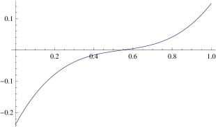
Figure 1: $x=1,t=0.1,\epsilon=0.01$, horizontal axis denote $\theta$, vertical axis denote the error

From Figure 1, in particular, assuming convergence-control parameter $\theta=0.5478$, one has

$$u_{t}+[F(u)u_{x}]_{x}+\epsilon u_{xxxx}\approx 4.70\times 10^{-6}.$$

II. $F=u$

We construct the following approximate solutions with fourth-order precision after assigning proper value to some parameters by ASM

$$u=\frac{x^{2}}{6t}+\frac{\epsilon}{x^{2}}-\frac{30\epsilon^{2}t}{x^{6}}-\frac{46440\epsilon^{3}t^{2}}{7x^{10}}-\frac{804646440\epsilon^{4}t^{3}}{203x^{14}}.$$

By virtue of the first five transformations of (20), a fourth-order approximate homotopy series solution follows

$$u=\frac{x^{2}}{6t}-\frac{\epsilon q(\theta-1)}{x^{2}}-\frac{\epsilon q^{2}(\theta-1)\left(390\epsilon(\theta-1)t+13\theta x^{4}\right)}{13x^{6}}$$

$$\hskip 22.76228pt+\frac{\epsilon q^{3}(\theta-1)\left(603720\epsilon^{2}(\theta-1)^{2}t^{2}-5460\epsilon\theta(\theta-1)tx^{4}-91\theta^{2}x^{8}\right)}{91x^{10}}$$

$$\hskip 22.76228pt+\epsilon q^{4}(\theta-1)\Big{[}\frac{-10460403720\epsilon^{3}(\theta-1)^{3}t^{3}+52523640\epsilon^{2}\theta(\theta-1)^{2}t^{2}x^{4}}{2639x^{14}}$$

$$\hskip 22.76228pt-\frac{237510\epsilon\theta^{2}(\theta-1)tx^{8}+2639\theta^{3}x^{12}}{2639x^{14}}\Big{]}.$$ (34)

When the constants and variables in solution (3.2) are specified by $x=1,t=0.1,\epsilon=0.01$, the relationship between the error of fourth-order precision approximate homotopy series solutions of (3.2) and parameter $\theta$ is sketched in Figure 2.

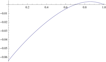
Figure 2: $x=1,t=0.1,\epsilon=0.01$, horizontal axis denote $\theta$, vertical axis denote the error

Especially, taking convergence-control parameter $\theta=0.7015$, one has

$$u_{t}+[F(u)u_{x}]_{x}+\epsilon u_{xxxx}\approx 1.59\times 10^{-6}.$$

4 Conclusion and discussion

In this paper, we show that the two couple equations derived by ASM and AHSM are connected by the transformation (20). As a result, approximate homotopy series solutions can be obtained by acting the transformation on the known solutions by ASM. As an application, the Cahn-Hilliard equation is considered to examine the results. This transformation may exert an important role in studying the perturbed PDEs because it makes researchers facilitate to study the results by AHSM through the ones by ASM.

In addition, it is worthwhile pointing out that, for Eq.(27), the unique pair of different operators $Y_{1},X_{1}$, i.e., the approximate homotopy symmetry operator

$$Y_{1}=-\frac{1}{2}x\partial_{x}-t\partial_{t}+\sum^{\infty}\limits_{i=1}\big{[}iu_{i}-(i-1)\theta u_{i-1}\big{]}\partial_{u_{i}}$$

and the corresponding approximate symmetry one

$$X_{1}=-\frac{1}{2}x\partial_{x}-t\partial_{t}+\sum\limits^{\infty}_{i=0}i\widetilde{u}_{i}\partial_{\widetilde{u}_{i}}$$

are equivalent under the transformation

$$u_{0}=\widetilde{u}_{0},~{}~{}~{}~{}u_{l}=\sum^{l-1}_{i=0}{l-1\choose i}\frac{l-i}{l}\,\theta^{i}\widetilde{u}_{l-i},~{}~{}l=1,2,\dots,$$

other than (20). Hence, the relations between the symmetries of two equivalent equations may form an interesting topic.

References

• [1] P.J. Olver, Applications of Lie Groups to Differential Equations, Springer, New York 1993.
• [2] G.W. Bluman and S. C. Anco, Symmetry and Integration Methods for Differential Equations, Springer, New York 2004.
• [3] V.A. Baikov, R.K. Gazizov, N.H. Ibragimov, Perturbation methods in group analysis, J. Soviet. Math. 55 (1991) 1450-1490.
• [4] W.I. Fushchich, W.H. Shtelen, On approximate symmetry and approximate solutions of the non-linear wave equation with a small parameter, J. Phys. A: Math. Gen. 22 (1989) L887-L890 .
• [5] M. Pakdemirli, M. Yurusoy, T. Dolapc, Comparison of Approximate Symmetry Methods for Differential Equations, Acta Appl. Math. 80 (2004) 243-271.
• [6] R. Wiltshire, Two approaches to the calculation of approximate symmetry exemplified using a system of advection-diffusion equations, J. Comput. Appl. Math. 197 (2006) 287-301.
• [7] X.Y. Jiao, Y. Gao, S.Y. Lou, Approximate homotopy symmetry method: Homotopy series solutions to the sixth-order Boussinesq equation, Sci. China. Ser. G-Phys. Mech. Astron. 52 (2009) 1169-1178.
• [8] Z.Y. Zhang, Y.F. Chen, A comparative study of approximate symmetry and approximate homotopy symmetry to a class of perturbed nonlinear wave equation, Nonlinear Anal. 74 (2011) 4300-4318.
• [9] J.W. Cahn, J.E. Hilliard, Free energy of a nonuniform system. I. Interfacial free energy, J. Chem. Phy. 28 (1958) 258-267.
• [10] X.D. Sun, M. J. Ward, Dynamics and Coarsening of Interfaces for the Viscous Cahn-Hilliard Equation in One Spatial Dimension, Stud. Appl. Math. 105 (2000) 203-234.
• [11] R.L. Mishkov, Generalization of the formula of Fa di Bruno for a composite function with a vector argument, Internat. J. Math.& Math. Sci. 24 (2000) 481-491.