SECULAR CHANGES IN ETA CARINAE’S WIND 1998–2011

Abstract

Stellar wind-emission features in the spectrum of eta Carinae have decreased by factors of 1.5–3 relative to the continuum within the last 10 years. We investigate a large data set from several instruments (STIS, GMOS, UVES) obtained between 1998 and 2011 and we analyze the progression of spectral changes in the direct view of the star, in the reflected polar-on spectra at FOS4, and at the Weigelt knots. We find that the spectral changes occurred gradually on a time scale of about 10 years and that they are dependent on the viewing angle. The line strengths declined most in our direct view of the star. About a decade ago, broad stellar wind-emission features were much stronger in our line-of-sight view of the star than at FOS4. After the 2009 event, the wind-emission line strengths are now very similar at both locations. High-excitation He I and N II absorption lines in direct view of the star strengthened gradually. The terminal velocity of Balmer P Cyg absorption lines now appears to be less latitude-dependent and the absorption strength may have weakened at FOS4. Latitude-dependent alterations in the mass-loss rate and the ionization structure of eta Carinae’s wind are likely explanations for the observed spectral changes.

1 INTRODUCTION

Eta Carinae, one of the most massive and most luminous stars in our Galaxy, is famous for its Great Eruption about 170 years ago. Its recovery has been unsteady with unexplained photometric and spectral changes in the 1890s and 1940s (Humphreys et al. 2008, and references therein). The spectral changes described in this paper may represent another rapid step in $\eta$ Car’s recovery from its Great Eruption.

Eta Car has a complex spectroscopic cycle, most likely regulated by a companion star in an eccentric orbit (Damineli et al. 1997, and many references in Humphreys & Stanek 2005 and Davidson & Humphreys 2012). So-called spectroscopic events occur every 5.54 years since 1948 (Feast et al., 2001; Damineli, 1996; Damineli et al., 2008b). The events are characterized by drastic changes in $\eta$ Car’s spectrum and photometry, e.g., high-excitation emission lines disappear for a few months (e.g., Gaviola 1953; Zanella et al. 1984) and light curves at all wavelength regions show significant variations (e.g., Whitelock et al. 1994; Corcoran et al. 1997; Feast et al. 2001; van Genderen et al. 2006; Fernández-Lajús et al. 2009; Martin & Koppelman 2004).

In a previous paper (Mehner et al., 2010b) we compared spectra at corresponding phases of successive spectroscopic cycles and found dramatic changes in observations after the 2009 event. Major stellar-wind emission features in the spectrum of $\eta$ Car had decreased by factors of order 2 relative to the continuum within 10 years and helium P Cyg absorption had become stronger. Most of the broad emission lines in $\eta$ Car’s spectrum originate in the primary star’s wind, see many papers and refs. in Humphreys & Stanek (2005), and the simplest explanation for the observed spectral changes is a decrease in $\eta$ Car’s wind density, by a factor of 2 or more. The early exit from $\eta$ Car’s 2009 X-ray minimum and the observed decrease of the 2–10 keV photons over the last two cycles are consistent with this interpretation (Kashi & Soker, 2009; Corcoran et al., 2010; Mehner et al., 2011b).

In this paper we analyze spectra obtained between 1998 and 2011 with several instruments to investigate in detail spectral changes in $\eta$ Car’s wind. We are not concerned here with the temporary spectral changes observed during the events – the spectral changes discussed are of secular nature. In Mehner et al. (2010b) we noted only a few examples; here we explore a wider range of effects, and whether or not they have developed gradually as opposed to sporadically. Section 2 describes the observations. In Section 3 we confirm the observations made by Mehner et al. (2010b) and show that the broad stellar wind features were still weak in HST STIS data obtained several months after our initial discovery in 2010 March data. The temporal progression of spectral changes and the dependence on the viewing direction is discussed. High-excitation emission and continuum from the nearby Weigelt knots, which are thought to be photoionized by a hot companion star, reveal additional information. In Section 4 we discuss the implications of these observations and estimate the decrease in mass-loss rate over the last 10 years. In Section 5 we give a short summary.

2 OBSERVATIONS AND DATA REDUCTION

To investigate the long-term recovery of $\eta$ Car from its Great Eruption, we need quantitative spectra with consistent instrument characteristics, sampled over several years. Unfortunately, no suitable data set exists prior to the Hubble Space Telescope (HST) observations. HST Space Telescope Imaging Spectrograph (STIS) observations in 1998–2004 and then again in 2009–2010 provide a consistent data set over a long time base-line. However, the STIS instrument was not available in 2004–2009, and the position FOS4 in the southeast (SE) lobe of the Homunculus, 4$\farcs$5 from the star, which shows the reflected pole-on spectrum was rarely observed with STIS. We therefore supplemented the STIS observations with ground-based data from the Very Large Telescope Ultraviolet and Visual Echelle Spectrograph (VLT UVES), the Gemini-South Gemini Multi-Object Spectrograph (Gemini GMOS), the Magellan II Magellan Inamori Kyocera Echelle (Magellan II MIKE), the Irénée du Pont Boller & Chivens Spectrograph (Irénée du Pont B&C), and the 1.5 m Cerro Tololo Interamerican Observatory Ritchey-Chrétien Spectrograph (1.5 m CTIO RC).

HST STIS/CCD spectra obtained with the 52″$\times$0$\farcs$1 slit in combination with the G230MB, G430M, and G750M gratings covered the wavelength region from $\lambda\lambda$1700–10,000 Å with spectral resolution $R\sim$ 5000–10,000. The observations include a variety of slit positions and orientations covering the entire Homunculus nebula, with a concentration at position angles $302^{\circ}$ and $332^{\circ}$ where the star and the nearby ejecta, called Weigelt knots B, C, and D, fall within the slit. The STIS data were reduced with improved reduction techniques that were developed for the Eta Carinae HST Treasury Program (Davidson, 2006). We extracted one-dimensional spectra with a sampling width of 0$\farcs$13 using a mesa function (Martin et al., 2006a) at positions which were observed regularly; the central star and the Weigelt knots C and D.

Gemini GMOS spectra of the central object and FOS4 obtained in 2007–2010 provide valuable supplemental and independent information. In most cases, we used the B1200 line grating at three tilt angles to cover the spectrum from $\lambda\lambda$3700–7500 Å. A 0$\farcs$5-wide slit, oriented with a position angle of 160^∘, was placed at different positions covering the star and FOS4. The resolving power was $R\sim$ 3000–6000. The data reduction was done using the standard GMOS data reduction pipeline in the Gemini IRAF package. The spectra were extracted using a mesa function 11 by 7 pixels wide, about 0$\farcs$8 by 0$\farcs$5. The seeing was roughly 0$\farcs$5–1$\farcs$5, so each GMOS spectrum discussed represents a region about 1″ across. The spectra were rectified using a LOESS fit.

Unfortunately, the observations with Gemini GMOS do not cover an entire spectroscopic cycle. Also, the important H$\alpha$ emission is so bright in $\eta$ Car that it saturates the detector pixels even in the shortest available GMOS exposures centered on the star. We therefore used observations obtained with the VLT UVES instrument to examine in particular H$\alpha$ from 2002 to 2009. The UVES observations are also extremely valuable because no other instrument covered the location at FOS4 consistently over such an extended time period. Eta Car was observed with UVES in the wavelength range from $\lambda\lambda$3000–8500 Å using 0$\farcs$3 and 0$\farcs$4-wide slits. The slits were oriented with constant slit position angle of 160^∘ and placed at two different positions covering the star and FOS4. The resolving power was $R\sim$ 80,000–110,000. The data were reduced with the standard UVES pipeline available from ESO. Spectra were extracted using a mesa function 3 by 2 pixels wide, about 0$\farcs$75 by 0$\farcs$5. The seeing was mostly between 0$\farcs$5 to 1$\farcs$5, with an average seeing of 0$\farcs$8.

The spatial resolution of the Gemini GMOS and VLT UVES observations, limited by atmospheric seeing, is greatly inferior to HST STIS spectra with spatial resolution better than 0$\farcs$2. In ground-based observations, the inner ejecta are unavoidably mixed with the spectrum of the star, and include the Weigelt knots 0$\farcs$3 northwest of the star. Fortunately, the slow-moving inner ejecta produce narrow emission lines which are distinguishable from the broad stellar wind lines. Typical widths are of the order of 20 and 400 km s^-1, respectively. At the wavelength region near $\lambda$4600 Å, which is of interest in our analysis, the spectral resolution is about 40 km s^-1 for STIS, roughly 75 km s^-1 for GMOS, and the UVES spectra have a spectral resolution better than 5 km s^-1. Narrow lines are therefore more blurred in the GMOS data while broad stellar wind features and their P Cyg absorption components are well resolved by all three instruments.

However, forbidden emission lines have an extended component at $\sim 0\farcs 2$ from the central source (Hillier et al., 2006). The blue emission with velocities of $-$200 to $-$400 km s^-1 is located elongated along the NE-SW axis southwards of the central source (Mehner et al., 2010a; Gull et al., 2011). The redshifted emission with velocities of $+$100 to $+$200 km s^-1 is more asymmetric and extends towards the north-northwest (Gull et al., 2011). These components are excluded in narrow extractions of the star in STIS observations but not in ground-based data which sample the inner $\sim 1\arcsec$ region. The broad stellar wind features near $\lambda$4600 Å, discussed in Section 3, normally include several forbidden lines and it is therefore non-trivial to compare HST with ground-based observations, see Section 3.1.

In 2010 June we obtained observations with Magellan II MIKE, covering a wavelength region between $\lambda\lambda$3200–10,000 Å. A 1″ slit was used which resulted in spectral resolutions $R\sim$ 22,000–28,000, or about 10 km s^-1 near $\lambda$4600 Å. The data were reduced with standard IRAF tasks and one-dimensional spectra corresponding to about 1″ on the sky were extracted.

In 2011 February, June, and December we also obtained spectra of $\eta$ Car and the FOS4 position with the B&C spectrograph at the Irénée du Pont telescope at Las Campanas Observatory. A 1″ slit was used with the 1200/4000 grating centered at $\lambda$4500 Å and the 1200/5000 grating centered at $\lambda$6000 Å, covering the wavelength range $\lambda\lambda$3700–6700 Å. The spectral resolution was $R\sim$ 2000–4000, or about 100 km s^-1 at $\lambda$4600 Å. The seeing varied between 1–2″. The data were reduced using standard IRAF tasks and spectra were extracted using a mesa function with peak width of 2 pixels and base width of 4 pixels, corresponding to 1$\farcs$4 and 2$\farcs$8.

We obtained low resolution spectra with the RC spectrograph on the SMARTS 1.5 m CTIO telescope in 2004–2012. A 2″ slit and grating #47 was used to cover the wavelength range $\lambda\lambda$5650–6970 Å with spectral resolution $R\sim$ 2000. A 2″ slit and grating #26 covered the wavelength range $\lambda\lambda$3660–5440 Å with spectral resolution $R\sim$ 1100. The data were reduced using standard procedures. Spectra are extracted by fitting a Gaussian plus a linear background at each column and represent a region of $\sim 2\arcsec$ on the sky.

We also used HST STIS/MAMA observations of the central star with grating E140M and slit width of 0$\farcs$2, obtained between 2000 March and 2004 March, to investigate $\eta$ Car’s terminal wind velocity during the 2003.5 event using the Si II $\lambda$1527 UV resonance line. The spectral resolution is $R\sim 100,000$. We extracted spectra using a mesa function, corresponding to 0$\farcs$13.

Throughout this paper we quote vacuum wavelengths and heliocentric Doppler velocities.

3 SPECTRAL CHANGES IN ETA CAR’S BROAD WIND-EMISSION FEATURES

In Mehner et al. (2010b) we reported dramatic changes in the broad wind-emission features of the central source in $\eta$ Car. We compared spectra at corresponding phases of successive cycles (phases 0.04 vs. 1.03, 1.12 vs. 2.10, and 0.21 vs. 2.20) and showed that the broad wind-emission features were considerably weaker in data obtained after the 2009 event, i.e., after phase 2.00, and that the He I absorption had become unusually strong. Observations with HST STIS obtained at phase 2.28 confirm these spectral changes, see Figure 1. The Figure shows spectral tracings of stellar wind features near $\lambda$4600 Å, H$\alpha$, and He I $\lambda$6680. In addition to the tracings at phases 0.21 (1999 February, $\sim 400$ days after the 1998 event) and 2.20 (2010 March 3, $\sim 400$ days after the 2009 event), which were already shown in Mehner et al. (2010b), the Figure includes observations at phase 2.28 (2010 August 20, $\sim 570$ days after the 2009 event). Between phases 2.21 and 2.28, the binary separation presumably increased by $\sim$ 14% while the orbital longitude changed by about $\sim 5^{\circ}$. STIS observations in 2010 October (phase 2.31) did not cover H$\alpha$ and He I $\lambda$6680 but sampled the broad wind features around $\lambda$4600 Å.

Figure 1a shows broad Fe II, [Fe II], Cr II, and [Cr II] emission blends near $\lambda$4600 Å which had decreased by a factor of 2–4 at phase 2.20 compared to phase 0.21. The strengths of the broad stellar wind features at phase 2.28 are comparable to the observations at phase 2.20. STIS observations at phase 2.31 confirm further the secular nature of the weakened emission strengths, see Table 1.

Figure 1b confirms that the profile of H$\alpha$ is altered and weakened in the recent STIS data. The narrow H$\alpha$ absorption near $-144$ km s^-1 seen in the tracing at phase 0.21 indicates unusual nebular physics far outside the wind (Johansson et al., 2005). This feature had weakened by 2007, reappeared during the 2009.0 event, but had practically vanished in March 2010 (Ruiz et al., 1984; Davidson et al., 1999b, 2005; Martin et al., 2010; Richardson et al., 2010). It is still absent in spectra obtained in 2011 December with Irénée du Pont B&C. The H$\alpha$ profile at phase 2.28 is very similar to the one at phase 2.20 but shows an additional small blue emission feature on top. This component probably indicates the same or adjoining material as observed in the shifting He I and N II emission lines (Mehner et al. 2011a, compare also with Figure 1c). Note that well after the 2009 event, H$\alpha$ showed no signs of resuming what had once been its “normal” appearance.

High-excitation He I emission did not weaken along with the features noted above, but the He I P Cyg absorption greatly strengthened after the 2009 event. In observations at phase 2.28 the absorption is still strong, see Figure 1c. STIS observation of He I $\lambda$4714 in 2010 October indicate that the helium absorption strengths may have even increased further compared to the 2010 August observations. He I emission and absorption lines shift to bluer wavelengths throughout $\eta$ Car’s spectroscopic cycle, compare tracings at phases 2.20 and 2.28 in the Figure (see also Nielsen et al. 2007 and Mehner et al. 2011b).

Overall, we find that observations obtained in 2010 August (phase 2.28) compare well with observations obtained in 2010 March (phase 2.20); the wind did not change substantially in-between these observations. This is further confirmed by the analysis of the few spectral features observed in 2010 October (phase 2.31). The spectral change since 2004 is thus not simply a peculiarity or aftermath of the 2009 event, but probably represents a significant secular development in $\eta$ Car’s wind. We discuss the long-term nature of the spectral changes and their implications in the next sections.

3.1 The Secular Character of the Spectral Changes

Spectral changes such as those found by Mehner et al. (2010b) were expected in the long-term recovery of $\eta$ Car  but it was generally assumed that they would occur much more slowly. The qualitative ground-based record from 1900 to 1990 showed no similar spectral changes in the broad wind-emission lines (excluding the events; see many refs. in Humphreys et al. 2008). During 1991–2004, HST Faint Object Spectrograph (FOS) and STIS spectra showed no obvious secular change in $\eta$ Car’s stellar wind spectrum. Figure 1a in Mehner et al. (2010b), illustrates the similarity of the broad wind features in two successive cycles before 2004 at phases 0.04 and 1.03. The 2009–2010 STIS data, however, revealed the weakest broad-line spectrum ever seen in modern observations of $\eta$ Car, relative to the underlying continuum. Low-excitation emission from the stellar wind became far less prominent on a time scale of only several years. We suggest that a decrease of $\eta$ Car’s mass-loss rate is the most probable explanation (Mehner et al., 2010b). A precedent may have been the appearance of the high-excitation lines in the 1940s, probably also due to a change in the wind density (Humphreys et al., 2008).

To determine whether $\eta$ Car’s spectrum changed only after – and as a result of – the 2009 event, or if, alternatively, the changes are of a more progressive nature, we investigated spectra obtained since 1998 with several instruments. The equivalent widths of two Fe II/Cr II blends near $\lambda$4600 Å in data from 1998–2012 are listed in Table 1. Ground-based observations, mainly with GMOS and UVES, fill in valuable data points during the years when STIS was unavailable, but they sample a wider region around the star and contain significant contributions from ejecta far outside the stellar wind and from the broad extended emission component of forbidden lines, such as [Fe II] and [Fe III], mentioned in Section 2. This results in very different equivalent width values for some broad wind features. Fortunately, several GMOS and UVES observations were obtained close to STIS observations, so we can correct for this effect as outlined below.

For example, on 2009 June 30 the equivalent width of the $\lambda\lambda$4570–4600 Å feature in STIS data was $EW$($\lambda\lambda$4570–4600,STIS) = $3.42\pm 0.27$ Å. In UVES spectra on 2009 June 30 the equivalent width is $EW$($\lambda\lambda$4570–4600,STIS) = $5.67\pm 0.38$ Å, a factor of 1.7 larger. Twenty four days later, on 2009 July 23, in GMOS spectra the equivalent width was $EW$($\lambda\lambda$4570–4600,GMOS) = $6.50\pm 0.31$ Å, a factor of 1.9 larger. Similarly, measurements for the blend at $\lambda\lambda$4614–4648 Å are 1.6 times larger in UVES and 1.8 times larger in GMOS spectra when compared to STIS spectra, see Table 1. UVES and GMOS observations overlap during the years 2008 and 2009 and we consistently find somewhat smaller equivalent widths in UVES spectra compared to GMOS spectra, probably due to their better spatial resolution. We use the 2009 June STIS data set, which mapped the inner 1″ region with slit offsets of 0$\farcs$1, to simulate a ground-based spectrum with a spatial sampling of 0$\farcs$65 by summing up the flux from the different slits. The equivalent widths from the simulated ground-based spectrum are; $EW$($\lambda\lambda$4570–4600,STIS,0.65”) $\approx 6.2$ Å and $EW$($\lambda\lambda$4614–4648,STIS,0.65”) $\approx 5.3$ Å. Those values agree well with the values obtained with UVES on the same day and the ones obtained about one month later with GMOS. The larger values found in ground-based data are therefore due to their larger spatial sampling.

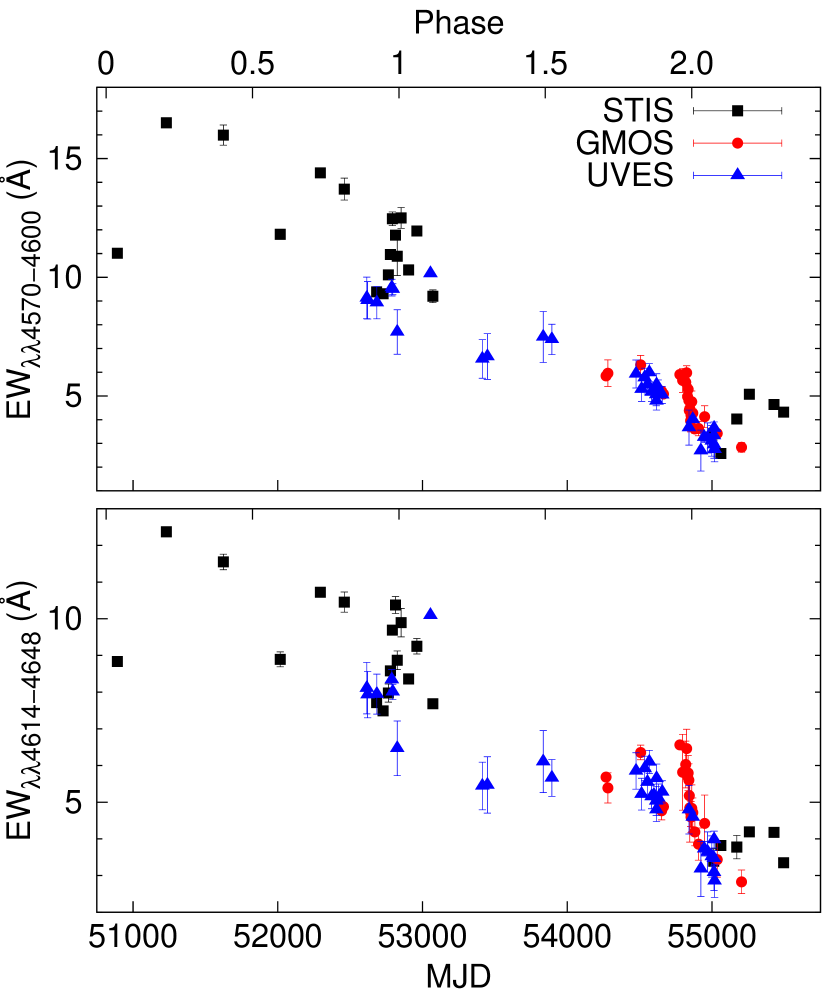
Figure 2: Equivalent widths of Fe II/Cr II blends at $\lambda\lambda$4570–4600 Å and $\lambda\lambda$4614–4648 Å  in HST STIS (black squares), Gemini GMOS (red circles), and VLT UVES (blue triangles) spectra in 1998–2010. Ground-based measurements were divided by 1.9 (GMOS, upper panel), 1.7 (UVES, upper panel), 1.8 (GMOS, lower panel), and 1.6 (UVES, lower panel) to account for the wider spatial sampling, see text. These broad stellar wind features show an almost linear decline over the last decade.

To compare the equivalent widths of the broad stellar wind features from different data sets, we adjust the values from the ground-based data using correction factors so that they are consistent with the values obtained from the STIS data in 2009. This approach may be questionable because 1) the inner and outer regions might not behave similar and 2) the 2009 data used to find the correction factors is very close to the 2009 event. However, our method is justified because following this procedure we find that the UVES values in 2002 to 2004 then also overlap with the STIS values during those years. We therefore account for the different spatial sampling of our ground-based data vs. the HST data by applying correction factors, see Figure 2 (applied factors are given in the Figure caption).

We find that the broad wind-emission features near $\lambda$4600 Å  decreased gradually by a factor of 2–3 over the last decade. Additional data sets, in particular the 1.5 m CTIO RC data, agree with this result, see Table 1. Neglecting observations close to $\eta$ Car’s spectroscopic events, near phases 1.0 and 2.0, when other factors dominate, the decline appears to be almost linear.

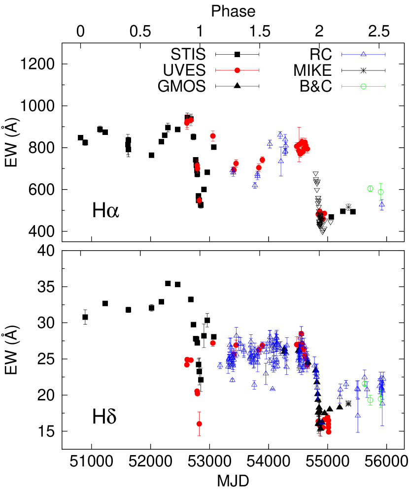
Figure 3: Equivalent width of H$\alpha$ and H$\delta$ in 1998–2012. HST STIS (black squares) observations, which unfortunately were not available in 2004–2009, are supplemented by VLT UVES (red circles), Gemini GMOS (filled black triangles), and Magellan II MIKE (star) data. Irénée du Pont B&C (green circle) and 1.5 m CTIO RC data (blue triangles) are of lower quality. The open black triangles are from 1.5 m CTIO RC and Echelle observations and are retrieved from Richardson et al. (2010). The H$\alpha$ and H$\delta$ minima were deeper during the 2009 event compared to the 2003.5 event and the line strength did not recover afterwards.

We also monitored the H$\alpha$ and H$\delta$ equivalent widths in observations since 1998, see Table 2 and Figure 3. HST STIS observations provide coverage over $\sim 12$ yr. In addition we analyzed data from the VLT UVES, Gemini GMOS, Magellan II MIKE, Irénée du Pont B&C, and 1.5 m CTIO RC spectrographs. H$\alpha$ equivalent width measurements during the 2009 event with the 1.5 m CTIO RC and Echelle spectrographs retrieved from Richardson et al. (2010) are also shown in the Figure. Unfortunately, H$\alpha$ could not be observed in direct view of the star with Gemini GMOS because the line is too bright even for the shortest allowed exposure times. No “correction” for different instruments as described above for the Fe II/Cr II blends is needed, since the total observed H$\alpha$ is dominated by the stellar wind contribution even in ground-based data.

Figure 3 shows a subtle long-term trend to smaller H$\alpha$ and H$\delta$ emission line strengths by a factor of $\sim 1.5$ over the last decade, but the decline appears to be more pronounced after the 2009 event. Between 1998 and 2003 (phases 0–1) the strengths of Balmer emission remained within $\pm 15\%$ of their median value. During the 2003.5 event, H$\alpha$ and H$\delta$ declined in $\sim 120$ days. H$\alpha$ then recovered in $\sim 200$ days and H$\delta$ faster in $\sim 120$ days. The 2009 event appeared, at first, to proceed similar to the previous event; the line strengths plummeted to a minimum in $\sim 120$ days. However, the minimum in 2009 was deeper than during the previous event and the emission did not recover to former strengths afterwards. A related note: Photometry at UV to visual wavelengths during the 2009 event also showed deeper minima in the light curves than in previous events (Fernández-Lajús et al., 2010; Mehner et al., 2011b). Davidson et al. (2005) had already reported significant differences in the hydrogen line profiles between the 1998 and 2003.5 events; each event is distinct. Outside the events, if we view only the data near phase $\sim 0.25$ of each cycle, then Figure 3 shows a linear trend somewhat like Figure 2. The gradual decrease of broad stellar wind-emission such as the Fe II/Cr II blends and hydrogen emission may represent a drop in $\eta$ Car’s mass-loss rate.

Teodoro et al. (2012) found no change in H$\delta$ line strength at phase $\sim 0.3$ in four consecutive cycles from 1994 to 2010. They argued that H$\delta$ is a better tracer of $\eta$ Car’s wind than, e.g., H$\alpha$ since it originates deep inside the primary’s wind and is therefore less affected by the wind-wind collision region. Finding no changes in the H$\delta$ profiles they concluded that no changes occured in $\eta$ Car’s mass loss rate but that the changes reported by Mehner et al. (2010b) were likely due to fluctuations in the wind-wind collision zone. However, Teodoro et al. only compared line profiles at one given phase and from two different data sets with inferior data quality than the data used in our analysis. Figure 3 shows that the trend described here is subtle and that individual measurements can fluctuate by up to $\sim 15\%$ within days. To investigate the longterm trend a consistent measurement over the last decade as presented here is needed.

Hydrogen P Cyg absorption in our direct line of view is basically absent during $\eta$ Car’s normal state, but strong P Cyg absorption develops for several months during the events (Smith et al., 2003), and was observed during the 2009 event (Richardson et al., 2010; Mehner et al., 2011b). Unfortunately, we were unable to obtain unsaturated H$\alpha$ profiles during the last event, but we did monitor H$\delta$ with GMOS. Before 2009 January only very weak H$\delta$ P Cyg absorption was observed. Strong absorption appeared suddenly between 2009 January 4 and 2009 January 9. In 2009 August STIS data the H$\alpha$ P Cyg absorption was absent but GMOS data still showed weak H$\delta$ P Cyg absorption in 2010 January.

Basic circumstances hamper the interpretation of $\eta$ Car’s Balmer absorption lines. Presumably they occur in zones where hydrogen is mostly ionized, since the associated emission lines are very strong and excitation to the $n=2$ level is difficult in H⁰ regions. Therefore they depend on the ratio $n(H^{0},n=2)/n(H^{+})$, which is small and sensitive to various effects that are hard to quantify for a complex asymmetric wind. Thus we cannot safely assume that a Balmer absorption strength is well correlated with gas density, for instance. These difficulties have led to a major interpretational disagreement between, e.g., Smith et al. (2003) and Richardson et al. (2010), as mentioned below.

The terminal velocity of H$\delta$ P Cyg absorption was $v_{\infty}\sim-550$ km s^-1 at all stellar latitudes in pre-event 2008 Gemini GMOS data (see Section 5 in Mehner et al. 2011b). During the event, the terminal velocity of hydrogen absorption lines increased in our direct line-of-sight to about $v_{\infty}\sim-900$ km s^-1. Smith et al. (2003) also found increasing terminal velocities of Balmer P Cyg absorption lines at moderate latitudes during the 1998 event. However, this does not necessarily imply that the velocity structure of $\eta$ Car’s wind changed. UV resonance lines are better suited to determine wind terminal velocities than Balmer lines. Unfortunately, no UV data were obtained during the 2009 event but HST STIS/MAMA covered $\eta$ Car from 2000 to 2004. Figure 4 compares Si II $\lambda$1527 in spectra of the star in our direct line-of-sight showing a constant terminal velocity of $\eta$ Car’s equatorial wind of $v_{\infty}\sim-600$ km s^-1. Only at phase 1.033 a higher wind velocity might be possible, but the spectrum shortward of $-600$ km s^-1 can also be explained by the general weakening of emission lines, visible in this same spectral region, during the event. The terminal velocity found in 1978 IUE data was comparable at $-600$ to $-700$ km s^-1 (Cassatella et al., 1979). The appearance of hydrogen absorption lines in our line-of-sight to $\eta$ Car and the increase of their terminal velocity may therefore result from changes in the ionization structure of $\eta$ Car’s wind modulated by the secondary star’s UV radiation (Richardson et al., 2010) or a wind cavity (Madura et al., 2011), and not from a change in the mass-loss structure as proposed by Smith et al. (2003).

Helium emission and absorption processes in $\eta$ Car’s wind depend on the companion star and have other special characteristics, see Section 6 of Humphreys et al. (2008). Similar to the case of a photoionized nebula, the amount of He I emission depends mainly on the hot companion star’s helium-ionizing photon output ($h{\nu}\gtrsim 25$ eV), with only weak dependences on the location of the recombining He⁺, gas density, and other details. Therefore it is not surprising that the helium emission lines behave differently from the lower-excitation features. The equivalent widths of He I emission lines remained constant from cycle to cycle. However, after the 2009 event, the He I P Cyg absorption strength had greatly increased compared to previous cycles (Mehner et al., 2010b). Groh & Damineli (2004) had already noted increasing He I $\lambda$6680 P Cyg absorption from 1992 to 2003. STIS observations since 1998 show that He I absorption in spectra in direct view of the central source was very weak shortly after the 1998 event, but increased until 2003. During the 2003.5 event, the absorption vanished, but reappeared shortly after. GMOS observations, starting in 2007 about 600 days before the 2009 event, show that the absorption increased further. It then again disappeared during the 2009 event but became very strong by mid-2009. Overall, the He I absorption strengths increased since 1998, only interrupted by episodes close to the events when the absorption disappeared for a few months. The same behavior is also observed for the N II $\lambda\lambda$5668–5712 series, discussed in Mehner et al. (2011a).

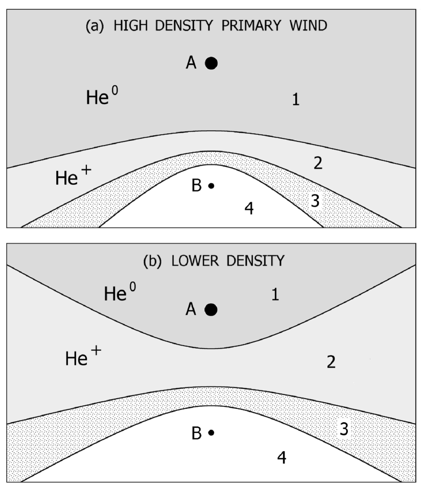
Figure 5: Schematic helium ionization zones in $\eta$ Car’s wind. A and B are the two stars. Zones 1 and 2 occur in the undisturbed primary wind, zone 3 is the colliding-wind shocked region, and zone 4 is the low-density secondary wind. Observed He I recombination emission arises mainly in zone 2, where helium is photoionized by the hot secondary star B. (Small condensations in zone 3 can also produce appreciable He I emission, but zone 4 is insufficiently dense.) The recent decrease of the primary wind may have enlarged the geometrical extent of zone 2 as shown in the bottom panel. Caveat: This diagram is highly idealized; for example, the boundary between zones 2 and 3 is quite unstable, irregular and ill-defined.

Changes in $\eta$ Car’s mass-loss rate help to explain these observations, because a lower wind density automatically implies larger photoionized zones. Since the observed He I absorption lines arise from highly excited levels, they are indirect consequences of recombination in He⁺ zones, not He⁰ (Osterbrock & Ferland, 2006); and the He⁺ gas is probably more extended than it was 10 years ago. Two plausible locations have been suggested, as sketched in Figure 5.

1. One is the shocked colliding-wind region, zone 3 in the figure (Humphreys et al., 2008; Damineli et al., 2008a). Most of the volume there has He⁺⁺ at $T>10^{6}$ K, but small cooled condensations also exist (see below). If they intercept most of the secondary star’s helium-ionizing photons, then they contain the relevant He⁺ gas, and zone 2 in Figure 5 shrinks to negligible thickness. In this case a change in the shocked zone, e.g., an increased opening angle, may explain the increasing He I P Cyg absorption (Groh et al., 2010b). In our view, the most likely reason for this to occur is a decrease in the primary wind outflow. This would move the shocked region closer to the primary star while broadening its opening angle – thus tending to increase the range of directions where a line of sight intersects appreciable He⁺.

2. On the other hand, as we explain below, the parameters strongly suggest that many of the secondary star’s ionizing photons pass between the small shocked-and-cooled condensations, penetrate into the primary wind, and form zone 2 in Figure 5. As the figure shows, this region becomes dramatically larger if the primary wind density decreases by a factor of three. The upper panel of the figure represents a dense wind, arguably like $\eta$ Car’s state before 2004. In that case, most geometric rays from the primary star do not intersect any He⁺ gas. With the orbit orientation favored by most authors (e.g., Okazaki et al. 2008; Parkin et al. 2009; Madura et al. 2012), our line of sight to the primary star would pass through the quasi-hyperboloidal He⁺ zone only for a limited time near conjunction, 3–11 months before periastron – depending of course on the orbit orientation and the shock-front opening angle. At other times, there would be little or no He⁺ along the line of sight. (The same statement applies to the shocked colliding-wind zone.) The lower panel of Figure 5, by contrast, has a far broader He⁺ zone because the wind is less dense by a factor of about 3. It notionally represents the situation today. In this case, our line of sight passes through He⁺ during most of the orbit, except for two or three months before and after periastron. Therefore a decreased wind density improves the observability of He I absorption, while having little effect on the He I emission strengths as we noted earlier.

In principle, zones 2 and 3 in Figure 5 may be of comparable importance for the He I lines. In both cases a decreased wind density appears to be consistent with the data.

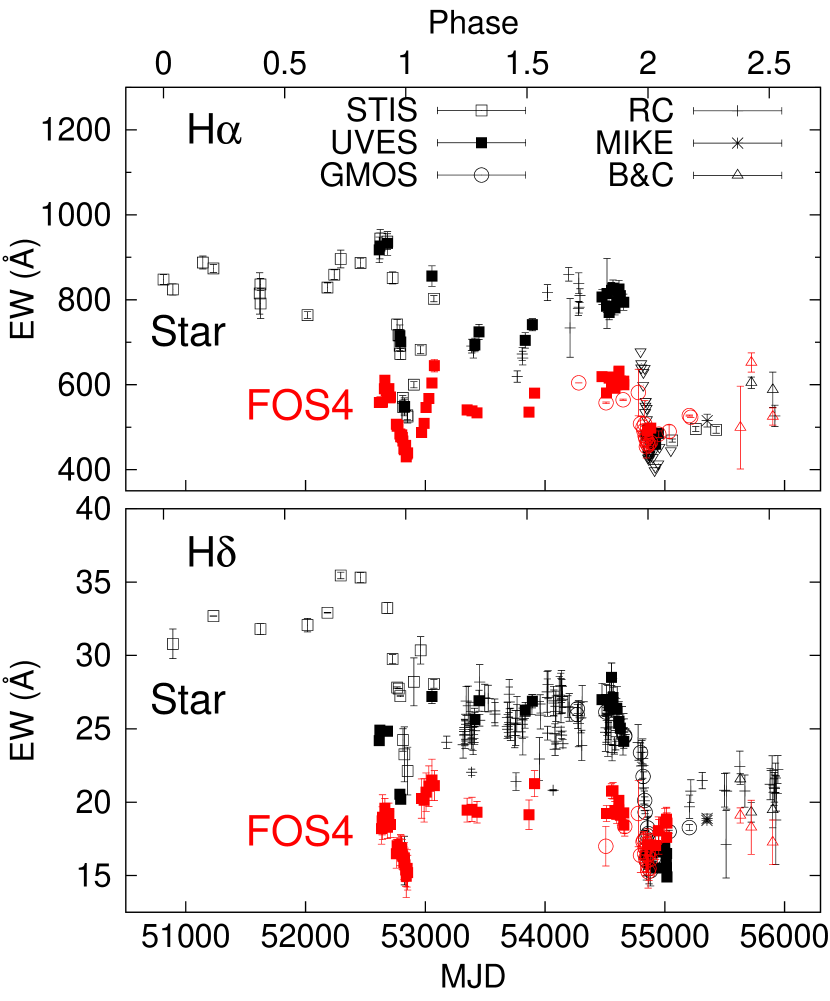
Figure 7: H$\alpha$ and H$\delta$ equivalent widths in spectra of the star in direct view (black symbols) and at FOS4 (red symbols) in spectra obtained in 1998–2012. (The open black triangles turned downwards are from 1.5 m CTIO RC and Echelle observations and are retrieved from Richardson et al. 2010.) The emission strengths decreased on the star by a factor of $\sim 1.5$ but not at FOS4.

Which of the above views is more accurate? Unfortunately the ionization problem is extremely intricate within the shocked gas. Consider, for example, the primary-wind shock at a time when it is located 15 AU from the primary star. For the sake of discussion, suppose the wind speed is 500 km s^-1, the total mass loss rate is $3\times 10^{-4}$ $M_{\odot}$ yr^-1, and ignore likely inhomogeneities in the wind. Then an idealized adiabatic shock produces post-shock temperature $T\sim 4\times 10^{6}$ K and electron density $n_{e}\sim 10^{9}$ cm^-3. But the cooling time is $t_{c}\sim 10^{5}$ s (Chapter 34 in Draine 2011), much faster than the outflow escape time $t_{esc}\sim 4\times 10^{6}$ s. Trapped X-rays may delay the cooling, but not enough to alter the basic situation. Therefore a naive one-dimensional shock model has a sheet of cooled gas with $T<$ 20,000 K. This gas is much denser than the pre-shock wind, because pressure equilibrium applies in an approximate sense between the two shock fronts. Consequently it would block practically all incident ionizing photons, so zone 2 in Figure 5 would not exist. This simple view is obviously unrealistic, though, because a number of well-known thermal, fluid, and radiation instabilities disrupt the sheet as rapidly as it forms. Figure 7 in Stevens et al. (1992) illustrates this phenomenon in a 2-dimensional model, and the case of $\eta$ Car is even more dramatic for two reasons: 3-dimensional geometry allows the development of small condensations, and the radiation pressure of ionizing radiation from the secondary star incites an additional, Rayleigh-Taylor-like instability. Hence there is little doubt that rapid cooling forms a fine spray of blob-like or filament-like condensations. Figure 7 in Stevens et al. hints that these may form streamers pointed toward the secondary star. Meanwhile, hot shocked gas between the condensations ($T\gtrsim 10^{6}$ K) contains He⁺⁺ and is nearly transparent to ionizing UV radiation. Evidently the question at hand is: Do the many small condensations intercept most of the UV photons incident on the shock structure? If they do, then He I emission and absorption arises mainly within the colliding-wind zone; but otherwise, zone 2 in our Figure 5 is more important.

Let us attempt an order-of-magnitude estimate with the same parameters assumed above. For simplicity we assume that each cooled condensation is a “blob” rather than a filament; if necessary a filament might be represented as a line of blobs. The characteristic pre-cooling size scale for thermal instability is of the order of $wt_{c}\sim 0.15$ AU, where $w\sim 200$ km s^-1 is the adiabatic-shocked sound speed. Cooling rapidly shrinks this size scale to less than 0.03 AU, about 1 percent of the colliding-wind region’s overall size scale. (The shrinkage factor is the cube root of the density-increase factor.) One expects roughly 300 blobs per AU³ (i.e., one per 0.15 AU cube) in the shocked region which is about 3 AU thick. Thus we expect a column density $N_{b}\sim 10^{3}$ blobs per AU². If the geometrical cross-section of each blob is $\sigma_{b}\sim(0.03\;\mathrm{AU})^{2}\sim 10^{-3}$ AU², then we find an “equivalent optical depth” $\tau_{b}=N_{b}\sigma_{b}\sim 1$, meaning that comparable numbers of photons either do or do not penetrate through the shocked region. Most of the factors neglected here would tend to decrease $\tau_{b}$. For instance, radiation pressure tends to either disrupt or ablate a blob on a time scale less than $t_{esc}$; and blobs may tend to be aligned with the direction to the secondary star, thereby increasing the transparency of regions between such filaments. In summary, the issue is left in doubt, because we can do only an order-of-magnitude assessment. No computer codes applied to $\eta$ Car so far can realistically solve this problem, because a satisfactory model requires (1) 3-dimensional fluid dynamics with spatial resolution $\sim\,10^{3}$, (2) realistic thermal and ionization microphysics including possible ablation, (3) realistic 3-dimensional radiative transfer for the ionizing photons, and (4) valid input parameters. None of these can be omitted. This puzzle is so intricate that tempting approximations may lead to serious errors. One interesting detail is that each condensation may move semi-ballistically, being too small and dense to follow the general fluid flow; while the ionizing-radiation pressure is not very much smaller than the thermal gas pressure. A final remark on this sub-topic: In view of the very strong instabilities of the primary-wind shock, exacerbated by inhomogeneities in the primary wind, the boundary between zones 2 and 3 in Figure 5 must be quite ill-defined and “fuzzy” at large and medium size scales.

3.2 Are Similar Spectral Changes Observed at Higher Stellar Latitudes?

Our line-of-sight to $\eta$ Car corresponds to stellar latitudes of about 45–50^∘ (Davidson et al., 2001; Smith et al., 2003) and as discussed above, spectra from this direct view show dramatic spectral changes over the past decade. The Homunculus nebula reflects light from the central source and allows us to view the star and its spectrum from different directions. The known geometry of the Homunculus makes it possible to directly relate locations in the nebula to stellar latitudes (Smith et al., 2003; Davidson et al., 2001; Zethson et al., 1999). Spectra at FOS4, located near the center of the SE lobe, correspond to a stellar latitude of about 75^∘ permitting us to observe the star’s spectrum from near its polar region. (Observed delay times and Doppler shifts confirm the assumed geometry, see Mehner et al. 2011b.) Spectra were obtained at FOS4 with VLT UVES from 2002–2009, with Gemini GMOS from 2007–2009, and with Irénée du Pont B&C in 2011.

Figure 6 shows the equivalent width of the Fe II/Cr II blend at $\lambda\lambda$4570–4600 Å on the star and at FOS4 with GMOS and UVES. In 2002–2003, the equivalent width of the emission in our direct view is a factor of $\sim 3$ larger than at FOS4. It was already noted by Hillier & Allen (1992) that the equivalent widths of emission lines are smaller throughout the lobes. This fact has not been fully explained, but one possible cause involves our unusual line-of-sight to the star. Our direct view of the star has more extinction than the Weigelt knots located only 0$\farcs$3 away (Davidson et al., 1995; Hillier et al., 2001). Suppose the extra obscuration occurs, for example, in a small intervening dusty cloud close to the star. Any extra emission formed between us and the cloud would have a magnified effect on the star’s apparent spectrum, because such emission would have less extinction. In that case, the star would appear to have relatively stronger emission lines than it really does. But this explanation has some obvious difficulties, and the problem is too complicated to explore here. See Smith et al. (2003) for other related comments. Stahl et al. (2005) and Weis et al. (2005) also noticed the difference but without discussion. The equivalent width in our direct view of the star declined by a factor of about 3 since 2002, while at FOS4 the decline was only by a factor of 1.5–2. After the 2009 event the strength of the emission feature was comparable at both locations.

Similar behavior is observed in the hydrogen emission lines. Figure 7 compares the H$\alpha$ and H$\delta$ equivalent widths in spectra of the star in direct view and reflected at FOS4 obtained with different instruments. The emission strength in spectra of the star decreased by a factor of $\sim 1.5$ since 1998 (see Section 3.1), but spectra at FOS4 showed no secular changes. After the 2009 event the emission strengths were about equal at both locations. Conceivably this is a hint that the wind has become more spherical.

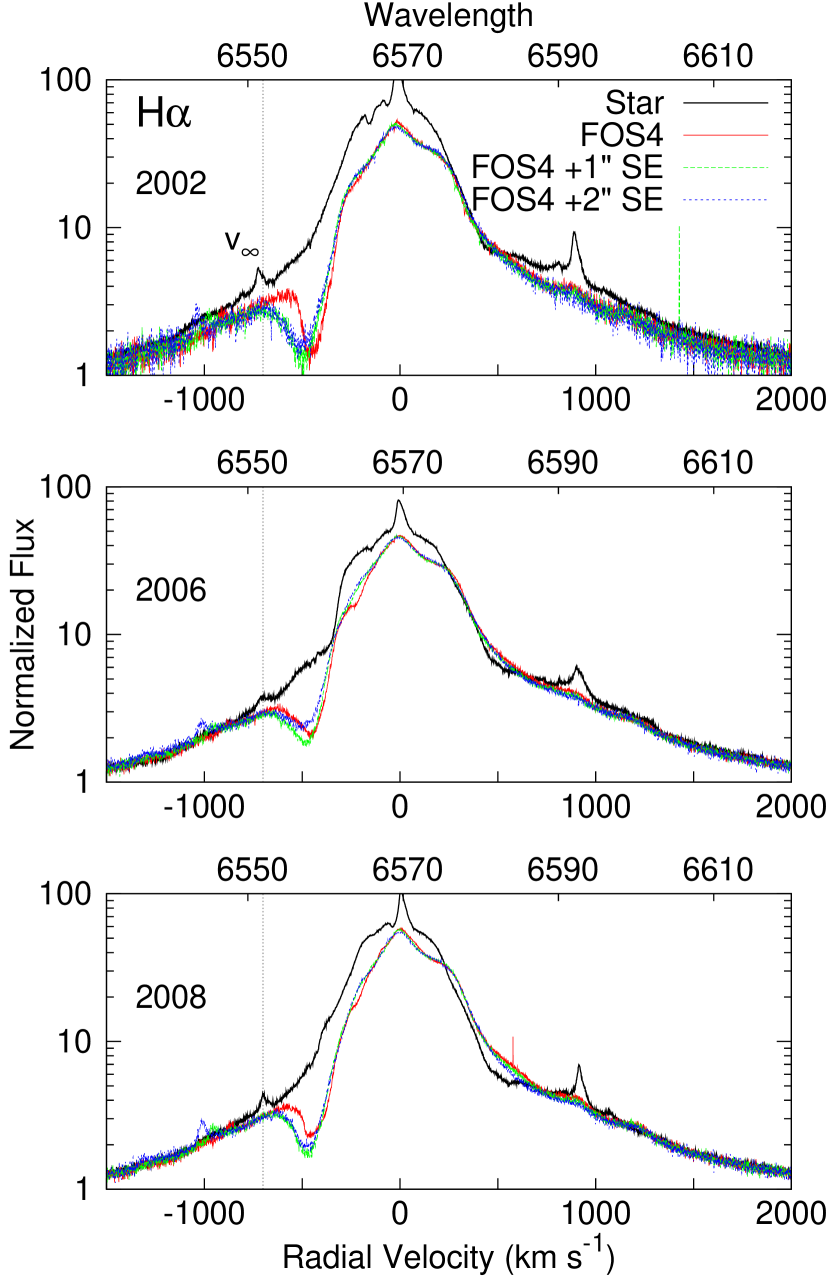
Figure 8: H$\alpha$ in VLT UVES spectra on the star and in the SE lobe. FOS4 +1″ and FOS4 +2″ are extraction along the slit 1″ and 2″ south of FOS4. Spectra were shifted by $-100$ km s^-1 (FOS4), $-150$ km s^-1 (FOS4 +1″) and $-200$ km s^-1 (FOS4 +2″) to account for the expanding nebula. Observations in 2002 and 2008 were obtained at similar phases (0.891 and 1.886). Tracings from 2006 show the mid-cyle profile. The maximum terminal velocity is $v_{\infty}\sim-700$ km s^-1 and the absorption feature may have weakened since 2002.

Smith et al. (2003) reported faster terminal velocities of Balmer P Cyg absorption lines at the poles than at lower latitudes in 2000 March STIS data during $\eta$ Car’s normal state, which lead them to conclude that $\eta$ Car’s wind is faster at the poles. They found terminal velocities of H$\alpha$ P Cyg absorption of $v_{\infty}=-540$ km s^-1 in our direct line-of-sight view and up to $v_{\infty}=-1150$ km s^-1 in the reflected polar-on spectra. In pre-2009 event ground-based data we did not find such high velocities at the poles. Observations with GMOS starting in 2007 show terminal velocities of the H$\delta$ absorption on the order of $v_{\infty}\sim-550$ km s^-1 at all latitudes (Mehner et al., 2011b). UVES observations $\sim 200$ days before the 2003.5 and 2009 events and during mid-cycle state in 2006 show that the maximum terminal velocities for H$\alpha$ increase somewhat with higher latitude and range from $v_{\infty}\sim-550$ to $v_{\infty}\sim-700$ km s^-1, see Figure 8. The telescope acquisition of the FOS4 location has an uncertainty of $\sim\pm 0.5{\arcsec}$ and this is the likely reason that the velocity dependence observed in the 2002 and 2008 spectra is not seen in the 2006 spectra shown in the Figure.

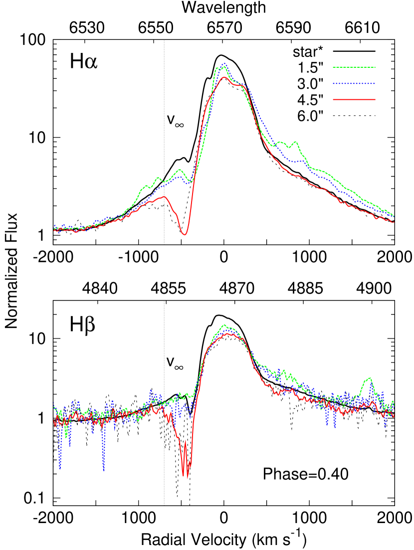
Figure 9: H$\alpha$ and H$\beta$ in 2000 March HST STIS observations in tracings along the SE lobe (the distance in arcsec from the central source is indicated). We corrected for the different redshifts using velocities of $-12$ km s^-1 for offset position 1$\farcs$5, $-43$ km s^-1 for offset position 3$\farcs$0, $-99$ km s^-1 for offset position 4$\farcs$5, and $-185$ km s^-1 for offset position 6$\farcs$0. The flux was normalized between $\lambda\lambda$6630–6650 Å and $\lambda\lambda$4980–5000Å, respectively. The terminal velocity is latitude-dependent, with the polar-on spectra showing the largest terminal velocities of $v_{\infty}\sim-700$ km s^-1.

Because we did not observe terminal velocities above $v_{\infty}=-700$ km s^-1 in our ground-based data, we reinvestigated the 2000 March STIS data used by Smith et al. (2003) using a different approach in aligning the spectra from several distinct locations in the Homunculus nebula. Smith et al. (2003) corrected for the different redshifts throughout the SE lobe, which are due to reflection by the expanding dust, by aligning the blue side of the H$\alpha$ emission line profile at 10 times the continuum flux. In Mehner et al. (2011b) we used, instead, several forbidden lines that are known to originate in the Weigelt knots with constant velocities much smaller than the discrepancy in question to align GMOS spectra. We cannot use the same procedure for the STIS spectra because the narrow lines cannot be as readily observed throughout the SE lobe due to the small spectral range of each exposure and the low S/N in extractions in the lobe. We therefore applied the velocities found for different locations in the SE lobe using GMOS data to the STIS spectra. The result is shown in Figure 9. Using our aligning method we found maximum terminal velocities of $v_{\infty}\sim-700$ km s^-1 for H$\alpha$ and H$\beta$. Admittedly $v_{\infty}$ is difficult to define precisely in a case like this. The lower two H$\alpha$ profiles in Figure 9 appear to show a deficit of flux between $-700$ and $-950$ km s^-1, but this is not a smooth continuation of the main P Cyg profile. Instead, these two examples are better described as having a possible weak second component of outflow with $v_{\infty}\sim-900$ km s^-1 rather than $-1150$ km s^-1. The H$\beta$ data are noisier, but this line produces deeper absorption than H$\alpha$; and it too shows no evidence for $v_{\infty}<-700$ km s^-1. Figure 9 shows a clear latitude dependence, but the velocity range is less dramatic than that found by Smith et al. (2003). Unfortunately, no UV observations of the reflected polar-on spectrum exist and we therefore cannot investigate the terminal velocities of UV resonance lines at higher latitudes.

Our last observations taken in 2010 January with GMOS and in 2011 with Irénée du Pont B&C indicate that the absorption at the poles had weakened considerably after the 2009 event. However, since the Irénée du Pont observations are of lower quality this has to be confirmed in future observations.

The simplest explanation for the weakening of broad stellar wind-emission features is a decrease in $\eta$ Car’s mass-loss rate (Mehner et al., 2010b). The broad stellar wind-emission features appear to be similar from all directions after the 2009 event suggesting that $\eta$ Car’s asymmetric wind (Smith et al., 2003) may have become more spherical over the last 10 years. If the interpretation of a decrease in mass-loss rate is correct, then the effect is latitude dependent with the mass-loss rate decreasing less or more slowly at the higher stellar latitudes. However, $\eta$ Car’s wind is normally assumed to be denser at the poles (Smith et al., 2003) and a larger decrease of the mass-loss rate at the equator would not lead to a more symmetric wind.

3.3 Are Spectral Changes Observed at the Weigelt Knots?

Spectra of the Weigelt knots show reflected light from $\eta$ Car and narrow high-excitation emission lines (Davidson et al., 1995) now attributed to photoionization by a hot companion star. Given the rapid spectral changes discussed above, and the accelerated brightening of the central star for the last 15 years (Martin & Koppelman, 2004; Martin et al., 2006b; Davidson et al., 2009), we expect to observe spectral changes also in the nearby ejecta. For instance, an early recovery of the high-excitation emission after the 2009 event and a larger continuum flux at the Weigelt knots seem reasonable. Unfortunately, the Weigelt knots cannot be spatially resolved in ground-based observations and their observational coverage with STIS is sparse; in 2003 the pre-event phase was covered, while the recovery phase was observed during the 1998 and 2009 events. Mid-cycle observations are even rarer.

Figure 10 shows measurements of the H$\alpha$ equivalent width at Weigelt knots C and D in STIS data for the last two cycles. Further observations are required to confirm the apparent long-term decrease in the emission strength of about 10–20%. Factors such as slightly varying slit position angles, pointing, and the fact that the knots are slowly moving outwards (on the order of 0$\farcs$023–0$\farcs$044 within 10 years, see Smith et al. 2004; Dorland et al. 2004) might play a role. We are not concerned here with the line behavior during the events, when the emission strength drops very rapidly for a few months.

Figure 11 shows the flux of the narrow [Ne III] $\lambda$3870 emission on Weigelt knots C and D since 1998 (compare Mehner et al. 2010a). High-excitation emission lines disappear for several months during the events, probably caused by the suppression of UV radiation from the secondary star close to periastron passage. Some authors have suggested that the disappearance of the high-excitation lines are caused by eclipses of a hot secondary star by the primary wind or wind-wind collision shock cone (Damineli et al., 1997; Ishibashi et al., 1999b; Stevens & Pittard, 1999; Pittard & Corcoran, 2002; Damineli et al., 2008a) or due to a thermal/rotational recovery cycle (Zanella et al., 1984; Davidson et al., 2000; Smith et al., 2003; Davidson, 2005). Many authors now agree that a collapse of the wind-wind collision structure (Davidson, 2002; Soker, 2003; Martin et al., 2006a; Soker & Behar, 2006; Soker, 2007; Damineli et al., 2008a), and/or disturbances in the primary wind (Davidson, 1997, 1999; Smith et al., 2003; Martin et al., 2006a), are primary causes for the observed spectral changes during the events. These phenomena can be triggered by the periastron passage of a companion star.

The [Ne III] $\lambda$3870 emission appears to have recovered faster after the 2009 than after the 1998 event. If $\eta$ Car’s wind has been decreasing in recent years, an early reappearance of the high-excitation emission lines would be expected since a lower mass-loss rate of the primary star would result in an earlier recovery of the secondary star’s UV radiation output in any proposed model. However, given the poor temporal coverage of the Weigelt knots this result is not conclusive.

Surprisingly, the continuum flux at $\sim\lambda$4000 Å at Weigelt knot D is very constant for the last 10 years, see Figure 12. The Figure compares the continuum flux at the star and at Weigelt knot D. Since the stellar continuum is much brighter than the continuum at knot D, we normalized the measurements to unity on 1998 March. In 1998, the stellar continuum at $\sim\lambda$4000 Å was $\sim 5$ times as bright as on the nearby knot D. The central source then brightened tremendously (see also Figure 1 in Mehner et al. 2011b for HST UV photometry). In 2010 August, the stellar continuum was about 60–70 times brighter than the continuum at knot D, which remained practically constant. This is quite unexpected. However, the rapid brightening of the central star is largely caused by a decrease in the circumstellar extinction; the innermost dust is being destroyed or the dust-formation rate has slowed. Our direct view of the star appears to have more circumstellar extinction than the average line-of-sight (Davidson et al., 1995) and the brightening of the central star may not be equal in all directions.

4 IMPLICATIONS FOR ETA CAR’S MASS-LOSS RATE

The spectral changes described in this paper suggest that $\eta$ Car’s wind density decreased and that the ionization structure of the inner wind changed. The changes appear to be dependent on the stellar latitude. Eta Car’s wind may be more spherical now than 10 years ago. However, the nature of these spectral changes cannot be easily explained.

In $\eta$ Car’s “normal” state, Balmer P Cyg absorption is strong at the poles and weak or absent along our line of sight, near stellar latitude $\sim$ 45^∘. It is therefore thought that $\eta$ Car’s wind density is higher at the poles (Smith et al., 2003), where it may resemble the spherical model described by Hillier et al. (2001). At lower latitudes, in this view, the wind is less dense, which implies stronger ionization and much weaker Balmer absorption. (The column density $N(H^{0},n=2)$ is small there because $N(H^{+}+H^{0})$ and the ratio $N(H^{0},n=2)/N(H^{+})$ are both smaller than they are at the poles.) A complex photoionization structure of the primary wind regulated by the secondary star (Richardson et al., 2010) or a wind cavity model (Madura et al., 2011) may provide additional or alternative explanations.

During the events, Balmer P Cyg absorption also appears at lower latitudes and the rapidly changing profiles indicate changes in $\eta$ Car’s wind ionization structure on very short time scales of only days. Smith et al. (2003) proposed that a minor mass ejection leads to a temporary increase in $\eta$ Car’s wind density in the equatorial regions resulting in hydrogen recombination. However, $\eta$ Car’s wind might be close to a regime where a small change in its wind parameters may lead to transitions between fully ionized and recombined hydrogen in the wind. This may be the case during the events, when the radiation of the secondary might cause a rapid transition between these two states and the ionization structure of $\eta$ Car’s wind might temporarily change (Richardson et al., 2010). Madura et al. (2011) found that a wind cavity in the dense primary wind caused by the secondary star may provide an explanation for the deepening of H$\alpha$ absorption in our line-of-sight during the events. Observations favoring the latter explanations are the constant terminal wind velocities in UV resonance lines during the 2003.5 event (see Figure 4) and the appearance of He I absorption at higher stellar latitudes for a few months before the 2009 event (Mehner et al., 2011b). UVES spectra before the 2003.5 event, starting at phase 0.9, show also strong He I absorption at the pole. This occurrence is not accounted for by a shell-ejection model.

The long-term weakening of H I emission in $\eta$ Car’s wind may be explained with a decrease in mass-loss rate, while the constant He I emission strength is probably due to competing effects of changes in the helium ionization, which is due mainly to UV from the hot companion star. Long-term changes in the H I and He I P Cyg absorption lines are related to changes in the ionization structure of $\eta$ Car’s wind and likely caused by alterations in the mass-loss rate. For example, Najarro et al. (1997) demonstrated that the variability of the H I and He I line profiles in P Cygni resulted from changes in the ionization of its wind.

Let us assume that the observed weakening of broad stellar wind features is primarily caused by a decreasing mass-loss rate, which seems natural for $\eta$ Car’s long-term recovery. A decrease in mass-loss rate is consistent with the accelerated secular brightening trend in HST images and spectroscopy (Davidson et al., 1999a; Martin & Koppelman, 2004; Martin et al., 2006b) as well as other recent observational evidence (Davidson et al., 2005; Martin et al., 2006b; Humphreys et al., 2008; Kashi & Soker, 2009; Martin et al., 2010; Corcoran et al., 2010).

Previous mass-loss rate estimates for $\eta$ Car range from $3\times 10^{-4}$ to $10^{-3}M_{\odot}$ yr^-1. Davidson et al. (1995) estimated the mass-loss rate based on the H$\beta$ emission line and found $6\times 10^{-4}$ to $3\times 10^{-3}M_{\odot}$ yr^-1, with a most likely value of $1\times 10^{-3}M_{\odot}$ yr^-1. Hillier et al. (2001) also found a mass-loss rate of $\sim 10^{-3}M_{\odot}$ yr^-1 by fitting the optical emission spectrum with a non-LTE line blanketed code. Radio observations at 8 and 9 GHz indicate mass-loss rates of $3\times 10^{-4}M_{\odot}$ yr^-1 (White et al., 1994) and millimeter observations resulted in $2.4\times 10^{-3}M_{\odot}$ yr^-1 (Cox et al., 1995). All those estimates are based on simplified, spherical models and are only order of magnitude estimates. Mass-loss rates obtained from optical observations are higher than from X-ray models, which find mass-loss rates of about $3\times 10^{-4}M_{\odot}$ yr^-1 (Ishibashi et al., 1999a; Corcoran et al., 2001; Pittard & Corcoran, 2002). This discrepancy might be reduced if clumping is taken into account since the mass-loss rates determined from $\rho^{2}$ diagnostics may have been systematically overestimated by up to an order of magnitude (Fullerton et al., 2006).

In this paper we did not attempt to estimate the absolute mass-loss rate of $\eta$ Car because there are too many unknowns such as the latitudinal dependence and clumping of the wind. Instead, we adopted the method by Leitherer (1988) which relates the H$\alpha$ luminosity to stellar mass-loss rate, stellar radius, velocity law, and effective temperature, to roughly estimate the change in mass-loss rate over the last 10 years. Assuming that only the mass-loss rate is responsible for the observed changes in H$\alpha$ flux, we find that the mass-loss rate declined by a factor of 2–3 between 1999 and 2010. Note: we do find absolute mass-loss rates on the right order of magnitude, i.e. $10^{-4}$–$10^{-3}~{}M_{\odot}$ yr^-1. A full theoretical analysis requires expert codes and new models updating Hillier et al. (2001) are needed.

A decrease in the mass-loss rate by a factor of 2–3 is consistent with estimates based on the X-ray light curve. The early exit from $\eta$ Car’s 2009 X-ray minimum suggests a decrease in mass-loss rate by a factor of 2 compared to previous events (Kashi & Soker, 2009). A decrease in mass loss rate by a factor of 2 also results from the decline in 2–10 keV X-ray flux by $\sim 30$% between 2000 and 2011. Corcoran et al. (2010) estimated a factor of 4 decrease in the mass loss rate between 2000 and 2006, which may be too excessive as the comparison was made based on the fluxes obtained nearly at a local maximum in 2000 and a local minimum in 2006. Corcoran et al. also suggested changes in the plasma temperature of the colliding wind shocks, which makes it difficult to assess what physical quantities – other than mass loss rate of $\eta$ Car – may have changed.

A decreasing mass-loss rate could also potentially explain the deepening of He I and N II absorption over the last decade. Eta Car’s wind may be in a stage where even a modest change in mass-loss rate can have a large impact on the wind ionization structure and a decrease in mass-loss rate may cause helium to become ionized in a larger fraction of the wind at low latitudes.

A dramatic drop in $\eta$ Car’s mass-loss rate mainly at the equatorial regions, however, leads to a significant conflict. Theories of equatorial gravity darkening in massive rotating stars (Maeder & Meynet, 2000; Maeder & Desjacques, 2001; Owocki, 2005) result in asymmetric winds with stellar wind densities and terminal wind velocities being larger at the poles, and the generally accepted hypothesis is that $\eta$ Car’s mass-loss rate was higher at the poles than at the equator (Smith et al., 2003). However, recent data imply a more spherical wind; the terminal velocities of Balmer P Cyg absorption appear to be fairly constant at all latitudes and emission strengths are equal from all directions. This cannot easily be explained alongside with a rapid decrease in mass-loss rate mainly at the equator. However, given the observational evidence presented above, the interpretation of a latitude-dependent wind caused by rapid stellar rotation might not be correct. Alternatives to the decreasing-wind interpretation include, e.g., a change in the latitude-dependence of the wind, changes in the velocity field shape, or the model favored by Kashi & Soker (2009), who propose that a small change in wind properties could be amplified by tidal interactions. More detailed analysis and future observations in the next years are necessary. We can only state here, that $\eta$ Car’s wind has changed considerably over the last decade but any explanation of the nature of these changes is not straightforward.

As noted in earlier papers, $\eta$ Car may now be returning to a state like that observed three centuries ago, with a nearly transparent wind (Martin et al., 2006b; Mehner et al., 2010b). Conceivably, however, it may already have reached that state. In 1998 its opaque wind had a pseudo-photospheric temperature of 9000–14,000 K (Hillier et al., 2001). Figure 1 in Davidson (1987) indicates that a factor of 2 or 3 decrease in the wind density should probably have raised the apparent temperature to 20,000 K or more. (Modernized opacities do not alter this relative statement.) According to an argument based on the star’s bolometric magnitude compared to the visual magnitude seen by Halley in 1677, the color temperature long before the Great Eruption was most likely about 20,000 to 25,000 K (Davidson, 2012). This value may represent either the star’s true effective temperature, or else a marginally opaque wind. If this reasoning is valid, perhaps the circumstellar extinction is the only remaining difference between the star’s appearance today and that seen 150 years before the Great Eruption. One implication is that the near-future development cannot safely be predicted merely by extrapolating from the past decade.

5 SUMMARY

In this paper we analyzed spectral data obtained with several instruments between 1998 and 2012. We confirmed the spectral changes in the wind emission lines first reported by Mehner et al. (2010b); HST STIS spectra obtained in 2010 August, $\sim 170$ days after the first discovery, are comparable to the observations in 2010 March. Furthermore, we analyzed the long-term development of spectral changes in our direct line-of-sight view of the star, at FOS4, and the Weigelt knots.

Eta Car’s recent spectral changes involve both emission and absorption lines:

1. Broad stellar wind-emission features in our line-of-sight to the star have decreased by factors of 1.5–3 relative to the continuum within the last 10 years. These changes occurred gradually and are dependent on the viewing angle; spectra at higher stellar latitudes and from the outlying ejecta show smaller changes. The simplest explanation is a decrease in $\eta$ Car’s primary wind density. However, the decrease in wind density appears to be latitude dependent, with emission features showing much less change at higher latitudes. After the 2009 event, emission line strengths are now very similar in our direct line-of-sight view and in the reflected polar-on spectrum at FOS4 suggesting a more spherical wind and/or a more uniform distribution of circumstellar extinction.

2. High-excitation He I and N II absorption lines strengthened gradually over the last decade indicating a change in $\eta$ Car’s wind ionization structure. Hydrogen P Cyg absorption at FOS4 might have weakened after the 2009 event. The terminal velocity of hydrogen P Cyg lines was found to be similar at all stellar latitudes. Those findings provide additional clues for a more spherical wind.

The observational results presented here are difficult to reconcile with a decrease in mass-loss rate primarily at lower stellar latitudes since it is generally assumed that $\eta$ Car’s wind had higher densities at the poles (Smith et al., 2003). Our observations may be more readily reconciled with alternative explanations for latitude-dependent spectral features, such as a complex ionization structure of $\eta$ Car’s wind modulated by the secondary star’s UV radiation (Richardson et al., 2010) or the presence of a wind cavity in the primary wind caused by the secondary star (Groh et al., 2010a; Madura et al., 2011).

Using H$\alpha$ emission and the method by Leitherer (1988) we found that $\eta$ Car’s mass-loss rate decreased by a factor of 2–3 between 1999 and 2010. A decrease in mass-loss rate on the order of 2–3 is consistent with changes in the X-ray light curve (Kashi & Soker, 2009; Corcoran et al., 2010). We did not attempt to derive the absolute value with any accuracy because there are too many unknown factors, such as latitudinal dependence and clumping of the wind. New theoretical models updating Hillier et al. (2001) are needed.

Observations in 2012 and 2013 will be extremely valuable to further analyze the nature of the spectral changes in $\eta$ Car’s wind. It is of great importance to monitor the star consistently since spectral changes may occur on time scales of only weeks to months. For the long-term recovery of $\eta$ Car it is important to investigate if the wind will further decline or if it will stabilize or even recover to its former strength. But by mid-2013, the onset of the next event will dominate the spectrum, so observations in 2012 are needed. The last three events all differed from each other and considering the long-term spectral changes described in this paper we can expect many interesting new results from $\eta$ Car’s 2014.5 event.

Acknowledgement We thank the staff and observers of the Gemini-South Observatory in La Serena for their help in preparing and conducting the observations, and Beth Perriello at STScI for assistance with HST observing plans. We also thank Otmar Stahl and Kerstin Weis for their effort in planning and obtaining the UVES spectra. AM was co-funded under the Marie Curie Actions of the European Commission (FP7-COFUND). MTR received partial support from Center for Astrophysics FONDAP and PB06 CATA (CONICYT).

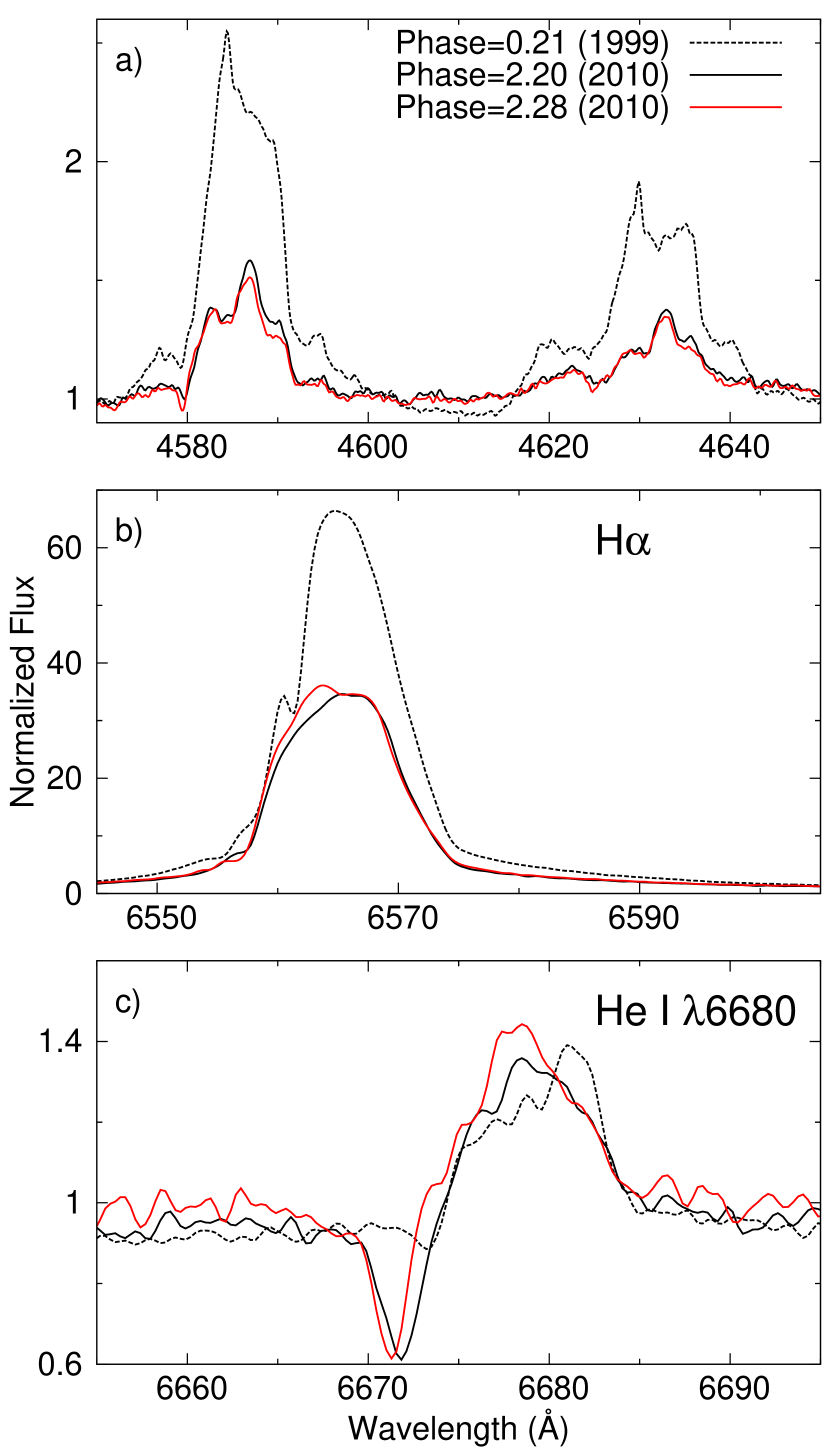
Figure 1: HST STIS spectral tracings about 400 days after the 1998 and the 2009 events (phases 0.21 and 2.20) and about 570 days after the 2009 event (phase 2.28); a) blends of Fe II, [Fe II], Cr II, and [Cr II] near $\lambda$4600 Å, flux is normalized to unity at $\lambda$4740 Å, b) H$\alpha$, flux is normalized to unity at $\lambda$6630 Å, c) He I $\lambda$6680, flux is normalized to unity at $\lambda$6630 Å. The strengths of broad wind-emission features have not recovered in 2010 August (phase 2.28) observations. The external narrow absorption near $-144$ km s^-1 in the H$\alpha$ profile is still absent. He I features shifted to bluer wavelengths and the He I P Cyg absorption is still strong at phase 2.28.

Figure 4: Si II $\lambda$1527 in HST STIS/MAMA observations in our direct line-of-sight to the central star. Phases are indicated next to each tracing and correspond to years 2000.23–2004.18. The terminal wind velocity in UV resonance absorption lines during the 2003.5 event is constant. The differing emission strengths seen in these tracings are related to $\eta$ Car’s spectroscopic cycle.

Figure 6: Equivalent width of the broad Fe II/Cr II blend at $\lambda\lambda$4570–4600 Å on the star (black symbols) and at FOS4 (red symbols) with Gemini GMOS and VLT UVES in 2002–2009. GMOS values were divided by 1.9 and UVES values by 1.7 to account for the wider spatial sampling, see text. The emission in our direct view of the star decreased by a factor of $\sim 3$, at FOS4 by only a factor of about 1.5–2.

Figure 10: Equivalent width of H$\alpha$ at the Weigelt knots C (filled squares) and D (open circles) over the last 2 cycles in HST STIS data. The equivalent width may have declined by about 10–20% over the last decade.

Figure 11: Flux of the narrow [Ne III] $\lambda$3870 emission line at Weigelt knots C (filled squares) and D (open circles) since 1998 in HST STIS data. The line strength may have recovered earlier after the 2009 event, see text.

Figure 12: Normalized continuum flux at $\lambda$3950 Å on the star (filled squares) and at Weigelt knot D (open circles). The flux was normalized to unity on 1998 March 19 for both locations. During $\eta$ Car’s last two spectroscopic cycles the continuum at $\lambda\sim 4000$ Å remained approximately constant at knot D, while the flux in our direct line of view rose by a factor of more than 10 between 1998 and 2010.

Table 1: Equivalent Widths of Broad Stellar Wind-emission Features (1998–2012)

Name	Date	MJD	Phase	EW${}_{\lambda\lambda 4570-4600\tablenotemark{c}}^{Star}$	EW${}_{\lambda\lambda 4614-4648\tablenotemark{c}}^{Star}$	EW${}_{\lambda\lambda 4570-4600\tablenotemark{c}}^{FOS4}$
	(UT)			(Å)	(Å)	(Å)
HST STIS
c821	1998 Mar 19	50891.4	0.038	11.02 $\pm$ 0.05	8.84 $\pm$ 0.01	$\cdots$
c914	1999 Feb 21	51230.5	0.206	16.51 $\pm$0.06	12.37 $\pm$ 0.10	$\cdots$
cA22	2000 Mar 20	51623.8	0.400	15.99 $\pm$ 0.42	11.55 $\pm$ 0.21	$\cdots$
cB29	2001 Apr 17	52016.8	0.595	11.81 $\pm$ 0.13	8.90 $\pm$ 0.21	$\cdots$
cC05	2002 Jan 20	52294.0	0.732	14.40 $\pm$ 0.06	10.73 $\pm$ 0.04	$\cdots$
cC51	2002 Jul 04	52459.5	0.813	13.72 $\pm$ 0.46	10.46 $\pm$ 0.28	$\cdots$
cD12	2003 Feb 13	52683.1	0.924	9.39 $\pm$ 0.01	7.72 $\pm$ 0.10	$\cdots$
cD24	2003 Mar 29	52727.3	0.946	9.31 $\pm$0.03	7.49 $\pm$ 0.11	$\cdots$
cD34	2003 May 05	52764.3	0.964	10.10 $\pm$ 0.07	7.98 $\pm$ 0.25	$\cdots$
cD37	2003 May 19	52778.5	0.971	10.96 $\pm$ 0.06	8.58 $\pm$ 0.04	$\cdots$
cD41	2003 Jun 01	52791.7	0.978	12.47 $\pm$ 0.29	9.69 $\pm$ 0.01	$\cdots$
cD47	2003 Jun 23	52813.8	0.989	11.78 $\pm$ 0.11	10.38 $\pm$ 0.23	$\cdots$
cD51	2003 Jul 05	52825.4	0.994	10.89 $\pm$ 0.81	8.87 $\pm$ 0.25	$\cdots$
cD58	2003 Aug 01	52852.4	1.008	12.50 $\pm$ 0.44	9.90 $\pm$ 0.39	$\cdots$
cD72	2003 Sep 22	52904.3	1.033	10.31 $\pm$ 0.10	8.36 $\pm$ 0.03	$\cdots$
cD88	2003 Nov 17	52960.6	1.061	11.95 $\pm$ 0.14	9.25 $\pm$ 0.21	$\cdots$
cE18	2004 Mar 07	53071.2	1.116	9.20 $\pm$ 0.27	7.69 $\pm$ 0.12	$\cdots$
cJ49	2009 Jun 30	55012.1	2.075	3.42 $\pm$ 0.27	3.39 $\pm$ 0.34	$\cdots$
cJ63	2009 Aug 19	55062.0	2.100	2.58 $\pm$ 0.21	3.82 $\pm$ 0.03	$\cdots$
cJ93	2009 Dec 06	55171.6	2.154	4.3 $\pm$ 0.15	3.78 $\pm$ 0.32	$\cdots$
cK16	2010 Mar 03	55258.6	2.197	5.07 $\pm$ 0.10	4.19 $\pm$ 0.12	$\cdots$
cK63	2010 Aug 20	55428.3	2.281	4.64 $\pm$ 0.18	4.18 $\pm$ 0.05	$\cdots$
cK81	2010 Oct 26	55495.1	2.314	4.32 $\pm$ 0.17	3.35 $\pm$ 0.01	$\cdots$
VLT UVES
uC93	2002 Dec 7	52615.3	0.890	15.52$\pm$1.49	12.97$\pm$1.21	$\cdots$
uC95	2002 Dec 12	52620.3	0.893	15.35$\pm$1.34	12.69$\pm$1.01	$\cdots$
uC98	2002 Dec 26	52634.4	0.900	$\cdots$	$\cdots$	4.80$\pm$0.10
uD00	2002 Dec 31	52639.3	0.902	$\cdots$	$\cdots$	5.15$\pm$0.06
uD00	2003 Jan 3	52642.3	0.904	$\cdots$	$\cdots$	5.05$\pm$0.09
uD05	2003 Jan 23	52662.4	0.914	$\cdots$	$\cdots$	5.74$\pm$0.05
uD09	2003 Feb 4	52674.4	0.920	$\cdots$	$\cdots$	5.28$\pm$0.02
uD12	2003 Feb 14	52684.1	0.924	15.18$\pm$1.16	12.71$\pm$0.87	5.12$\pm$0.09
uD15	2003 Feb 25	52695.3	0.930	$\cdots$	$\cdots$	4.92$\pm$0.03
uD18	2003 Mar 12	52710.0	0.937	$\cdots$	$\cdots$	5.08$\pm$0.01
uD33	2003 Apr 30	52759.1	0.962	$\cdots$	$\cdots$	4.73$\pm$0.07
uD33	2003 May 5	52765.0	0.964	$\cdots$	$\cdots$	5.60$\pm$0.02
uD36	2003 May 12	52771.2	0.967	$\cdots$	$\cdots$	5.75$\pm$0.10
uD40	2003 May 29	52788.1	0.976	16.26$\pm$0.60	13.34$\pm$0.44	4.90$\pm$0.11
uD42	2003 Jun 3	52794.0	0.979	16.14$\pm$0.39	12.81$\pm$0.33	5.11$\pm$0.11
uD42	2003 Jun 8	52798.0	0.981	$\cdots$	$\cdots$	5.26$\pm$0.06
uD45	2003 Jun 13	52803.0	0.983	$\cdots$	$\cdots$	5.42$\pm$0.08
uD45	2003 Jun 17	52808.0	0.986	$\cdots$	$\cdots$	5.18$\pm$0.15
uD47	2003 Jun 22	52813.0	0.988	$\cdots$	$\cdots$	5.68$\pm$0.32
uD49	2003 Jun 30	52821	0.992	$\cdots$	$\cdots$	5.03$\pm$0.24
uD51	2003 Jul 5	52825.0	0.994	13.08$\pm$1.59	10.35$\pm$1.19	6.65$\pm$1.02
uD51	2003 Jul 9	52830.0	0.997	$\cdots$	$\cdots$	5.25$\pm$0.37
uD54	2003 Jul 21	52841.0	1.002	$\cdots$	$\cdots$	3.78$\pm$0.52
uD57	2003 Jul 27	52848.0	1.005	$\cdots$	$\cdots$	5.91$\pm$1.28
uD57	2003 Aug 1	52852.0	1.007	$\cdots$	$\cdots$	3.47$\pm$0.73
uD90	2003 Nov 25	52968.3	1.065	$\cdots$	$\cdots$	4.00$\pm$0.45
uD96	2003 Dec 17	52990.3	1.076	$\cdots$	$\cdots$	4.29$\pm$0.50
uE00	2004 Jan 2	53006.3	1.084	$\cdots$	$\cdots$	4.47$\pm$0.38
uE07	2004 Jan 25	53029.3	1.095	$\cdots$	$\cdots$	3.88$\pm$0.29
uE14	2004 Feb 20	53055.1	1.108	17.27$\pm$0.08	16.15$\pm$0.06	3.77$\pm$0.27
uE19	2004 Mar11	53075.1	1.118	$\cdots$	$\cdots$	3.90$\pm$0.55
uE94	2004 Dec 10	53349.3	1.253	$\cdots$	$\cdots$	4.33$\pm$0.11
uF05	2005 Jan 19	53389.2	1.273	$\cdots$	$\cdots$	4.28$\pm$0.26
uF12	2005 Feb 12	53413.4	1.285	11.15$\pm$1.38	8.71$\pm$1.04	$\cdots$
uF17	2005 Mar 2	53431.3	1.294	$\cdots$	$\cdots$	4.57$\pm$0.18
uF21	2005 Mar 19	53448.1	1.302	11.32$\pm$1.64	8.75$\pm$1.23	$\cdots$
uG27	2006 Apr 9	53834.1	1.493	12.72$\pm$1.82	9.77$\pm$1.35	$\cdots$
uG36	2006 May 11	53866.0	1.509	$\cdots$	$\cdots$	4.92$\pm$0.31
uG43	2006 Jun 8	53894.0	1.523	12.55$\pm$1.09	9.06$\pm$0.80	$\cdots$
uG48	2006 Jun 26	53912.1	1.531	$\cdots$	$\cdots$	5.39$\pm$0.30
uI02	2008 Jan 10	54475.3	1.810	10.07$\pm$1.01	9.36$\pm$0.79	$\cdots$
uI13	2008 Feb 17	54513.3	1.829	8.99$\pm$0.88	8.35$\pm$0.69	3.44$\pm$0.13
uI19	2008 Mar 10	54535.3	1.839	9.81$\pm$0.67	9.47$\pm$0.53	$\cdots$
uI24	2008 Mar 29	54554.3	1.849	9.30$\pm$0.67	8.88$\pm$0.53	3.61$\pm$0.16
uI28	2008 Apr 11	54567.0	1.855	10.17$\pm$0.64	9.76$\pm$0.51	3.58$\pm$0.05
uI32	2008 Apr 27	54583.0	1.863	8.78$\pm$0.67	8.24$\pm$0.53	3.33$\pm$0.15
uI36	2008 May 12	54599.0	1.871	8.84$\pm$0.01	8.31$\pm$0.01	3.58$\pm$0.16
uI41	2008 May 28	54615.0	1.879	8.59$\pm$0.80	8.06$\pm$0.64	$\cdots$
uI41	2008 May 30	54616.0	1.879	8.14$\pm$0.65	7.67$\pm$0.52	4.11$\pm$0.12
uI41	2008 May 31	54617.1	1.880	9.31$\pm$0.79	9.03$\pm$0.63	3.61$\pm$0.13
uI44	2008 Jun 11	54629.0	1.886	8.88$\pm$0.77	8.19$\pm$0.61	3.61$\pm$0.10
uI52	2008 Jul 9	54656.0	1.899	8.58$\pm$0.61	8.45$\pm$0.49	3.93$\pm$0.08
uI52	2008 Jul 10	54657.1	1.900	$\cdots$	$\cdots$	3.51$\pm$0.14
uJ03	2009 Jan 10	54841.4	1.991	6.23$\pm$1.26	7.67$\pm$1.06	$\cdots$
uJ07	2009 Jan 25	54856.2	1.998	$\cdots$	$\cdots$	2.65$\pm$0.19
uJ10	2009 Feb 5	54867.3	2.004	6.82$\pm$0.01	7.35$\pm$0.01	$\cdots$
uJ14	2009 Feb 20	54882.2	2.011	$\cdots$	$\cdots$	1.23$\pm$0.46
uJ25	2009 Apr 2	54923.2	2.031	4.59$\pm$1.47	5.09$\pm$1.21	0.82$\pm$0.00
uJ31	2009 Apr 25	54946.1	2.043	5.55$\pm$0.39	5.96$\pm$0.31	1.09$\pm$0.02
uJ38	2009 May 19	54970.0	2.054	5.49$\pm$1.08	5.83$\pm$0.88	1.83$\pm$0.02
uJ46	2009 Jun 17	54999.1	2.069	5.28$\pm$1.09	5.63$\pm$0.90	3.18$\pm$0.72
uJ50	2009 Jun 30	55013.0	2.076	5.67$\pm$0.38	5.55$\pm$0.33	4.17$\pm$0.29
uJ50	2009 Jul 1	55014.0	2.076	5.02$\pm$0.98	4.94$\pm$0.80	1.73$\pm$0.17
uJ50	2009 Jul 2	55015.0	2.077	6.20$\pm$0.44	6.37$\pm$0.37	3.26$\pm$0.07
uJ51	2009 Jul 5	55018.0	2.078	4.68$\pm$0.90	4.57$\pm$0.73	1.63$\pm$0.06
Gemini GMOS
gH45	2007 Jun 16	54268.0	1.707	11.10 $\pm$ 0.20	10.23 $\pm$ 0.19	$\cdots$
gH49	2007 Jun 30	54281.0	1.714	11.32 $\pm$ 1.07	9.70 $\pm$ 0.74	4.23$\pm$0.21
gI11	2008 Feb 11	54507.4	1.826	11.99 $\pm$ 0.76	11.44 $\pm$ 0.36	4.02$\pm$0.22
gI50	2008 Jul 05	54652.0	1.897	9.88 $\pm$ 0.10	8.58 $\pm$ 0.45	4.01$\pm$0.04
gI54	2008 Jul 17	54665.0	1.904	9.65 $\pm$ 0.04	8.78 $\pm$ 0.03	3.92$\pm$0.00
gI85	2008 Nov 08	54778.3	1.960	11.21 $\pm$ 0.00	11.81 $\pm$ 0.00	3.86$\pm$0.36
gI90	2008 Nov 27	54797.3	1.969	10.74 $\pm$ 0.96	10.47 $\pm$ 1.86	3.83$\pm$0.10
gI96	2008 Dec 18	54818.3	1.979	10.60 $\pm$ 1.03	10.85 $\pm$ 1.15	3.67$\pm$0.20
gI98	2008 Dec 25	54825.3	1.983	11.35 $\pm$ 0.57	11.63 $\pm$ 0.95	3.59$\pm$0.26
gI99	2008 Dec 31	54831.3	1.986	9.44 $\pm$ 0.38	10.26 $\pm$ 0.14	3.50$\pm$0.28
gJ01	2009 Jan 04	54835.3	1.988	10.03 $\pm$ 0.38	10.43 $\pm$ 0.86	3.47$\pm$0.53
gJ02	2009 Jan 09	54840.2	1.990	9.14 $\pm$ 0.54	10.08 $\pm$ 0.80	3.17$\pm$0.43
gJ03	2009 Jan 12	54843.3	1.992	8.33 $\pm$ 0.28	9.32 $\pm$ 0.08	3.49$\pm$0.44
gJ04	2009 Jan 15	54846.2	1.993	8.48 $\pm$ 1.42	8.72 $\pm$ 1.68	3.24$\pm$0.30
gJ05	2009 Jan 21	54852.3	1.996	7.51 $\pm$ 0.88	8.49 $\pm$ 0.69	2.95$\pm$0.22
gJ06	2009 Jan 24	54855.3	1.998	7.94 $\pm$ 0.52	8.27 $\pm$ 0.77	3.08$\pm$0.42
gJ07	2009 Jan 29	54860.4	2.000	9.04 $\pm$ 0.85	8.70 $\pm$ 1.15	3.63$\pm$0.34
gJ09	2009 Feb 05	54867.2	2.004	8.12 $\pm$ 0.33	8.49 $\pm$ 0.72	3.52$\pm$0.11
gJ13	2009 Feb 19	54881.2	2.011	6.86 $\pm$ 0.36	7.54 $\pm$ 0.68	2.94$\pm$0.51
gJ20	2009 Mar 17	54907.3	2.023	6.89 $\pm$ 0.58	6.94 $\pm$ 0.79	$\cdots$
gJ32	2009 Apr 28	54949.1	2.044	7.84 $\pm$ 0.87	7.96 $\pm$ 1.39	2.39$\pm$0.42
gJ56	2009 Jul 23	55036.0	2.087	6.50 $\pm$ 0.31	6.18 $\pm$ 0.86	2.89$\pm$0.76
gK02	2010 Jan 08	55204.3	2.170	5.39 $\pm$ 0.39	5.09 $\pm$ 0.58	$\cdots$
gK05	2010 Jan 20	55216.3	2.176	$\cdots$	$\cdots$	2.74$\pm$0.01
Magellan II MIKE
$\cdots$	2010 Jun 4	55352.62	2.244	6.95$\pm$0.36	3.84$\pm$0.55	$\cdots$
Irénée du Pont B&C
$\cdots$	2011 Feb 25	55629.92	2.381	6.48$\pm$0.12	4.94$\pm$0.08	3.49$\pm$0.48
$\cdots$	2011 Jun 8	55720.95	2.426	4.42$\pm$0.417	5.05$\pm$0.38	3.12$\pm$0.30
$\cdots$	2011 Dec 5	55900.3	2.514	4.62$\pm$0.63	5.31$\pm$0.56	2.06$\pm$0.66
1.5 m CTIO RC
$\cdots$	2004 Jun 22	53178.1	1.169	10.51$\pm$1.15	8.56$\pm$0.84	$\cdots$
$\cdots$	2004 Nov 6	53315.4	1.236	9.02$\pm$0.84	7.39$\pm$0.63	$\cdots$
$\cdots$	2004 Nov 17	53326.3	1.242	10.84$\pm$1.31	8.15$\pm$1.33	$\cdots$
$\cdots$	2004 Nov 18	53327.4	1.242	10.37$\pm$1.85	7.94$\pm$1.34	$\cdots$
$\cdots$	2004 Nov 19	53328.3	1.243	10.47$\pm$1.49	8.06$\pm$1.08	$\cdots$
$\cdots$	2004 Nov 20	53329.3	1.243	10.53$\pm$1.96	8.33$\pm$1.43	$\cdots$
$\cdots$	2004 Nov 22	53331.3	1.244	10.32$\pm$1.00	7.71$\pm$0.73	$\cdots$
$\cdots$	2004 Dec 2	53341.3	1.249	10.79$\pm$0.65	8.62$\pm$0.48	$\cdots$
$\cdots$	2004 Dec 19	53358.4	1.258	10.64$\pm$1.05	8.49$\pm$0.78	$\cdots$
$\cdots$	2005 Jan 2	53372.3	1.265	10.64$\pm$1.36	7.56$\pm$0.96	$\cdots$
$\cdots$	2005 Jan 3	53373.4	1.265	10.70$\pm$1.36	8.01$\pm$1.00	$\cdots$
$\cdots$	2005 Jan 13	53383.4	1.270	11.11$\pm$1.21	8.05$\pm$0.87	$\cdots$
$\cdots$	2005 Jan 14	53384.2	1.271	11.00$\pm$1.35	8.02$\pm$0.97	$\cdots$
$\cdots$	2005 Jan 15	53385.3	1.271	10.03$\pm$1.12	7.29$\pm$0.80	$\cdots$
$\cdots$	2005 Jan 28	53398.3	1.277	10.92$\pm$1.17	8.02$\pm$0.84	$\cdots$
$\cdots$	2005 Jan 29	53399.3	1.278	10.31$\pm$1.38	7.65$\pm$1.01	$\cdots$
$\cdots$	2005 Feb 9	53410.4	1.283	10.90$\pm$1.12	7.98$\pm$0.81	$\cdots$
$\cdots$	2005 Feb 10	53411.4	1.284	10.81$\pm$0.79	7.97$\pm$0.57	$\cdots$
$\cdots$	2005 Mar 25	53454.1	1.305	10.56$\pm$1.01	8.55$\pm$0.75	$\cdots$
$\cdots$	2005 Mar 26	53455.2	1.306	10.79$\pm$0.75	8.42$\pm$0.55	$\cdots$
$\cdots$	2005 May 6	53496.1	1.326	10.83$\pm$1.36	7.77$\pm$0.98	$\cdots$
$\cdots$	2005 Jun 4	53525.1	1.340	10.71$\pm$0.94	7.97$\pm$0.68	$\cdots$
$\cdots$	2005 Jul 28	53580.0	1.367	9.87$\pm$1.44	7.61$\pm$1.05	$\cdots$
$\cdots$	2005 Jul 30	53582.0	1.368	9.93$\pm$0.97	7.90$\pm$0.72	$\cdots$
$\cdots$	2005 Nov 10	53684.4	1.419	10.63$\pm$1.22	7.37$\pm$0.87	$\cdots$
$\cdots$	2005 Nov 11	53685.4	1.419	10.95$\pm$1.30	7.95$\pm$0.93	$\cdots$
$\cdots$	2005 Nov 13	53687.3	1.420	10.87$\pm$1.33	7.82$\pm$0.95	$\cdots$
$\cdots$	2005 Nov 24	53698.4	1.426	10.33$\pm$1.46	7.08$\pm$1.05	$\cdots$
$\cdots$	2005 Nov 26	53700.4	1.427	10.78$\pm$1.73	7.71$\pm$1.24	$\cdots$
$\cdots$	2005 Nov 27	53701.3	1.427	10.90$\pm$1.88	7.79$\pm$1.35	$\cdots$
$\cdots$	2005 Dec 7	53711.3	1.432	11.18$\pm$1.59	7.93$\pm$1.15	$\cdots$
$\cdots$	2006 Jan 11	53746.3	1.449	9.46$\pm$1.85	6.92$\pm$1.34	$\cdots$
$\cdots$	2006 Jan 16	53751.2	1.452	11.36$\pm$1.46	7.92$\pm$1.04	$\cdots$
$\cdots$	2006 Jan 19	53754.3	1.453	10.84$\pm$1.55	7.36$\pm$1.09	$\cdots$
$\cdots$	2006 Jan 29	53764.2	1.458	11.73$\pm$1.57	8.12$\pm$1.14	$\cdots$
$\cdots$	2006 Jan 31	53766.2	1.459	11.63$\pm$1.79	8.28$\pm$1.28	$\cdots$
$\cdots$	2006 Mar 14	53808.1	1.480	11.77$\pm$1.32	8.04$\pm$0.94	$\cdots$
$\cdots$	2006 Mar 16	53810.1	1.481	11.34$\pm$1.13	7.94$\pm$0.82	$\cdots$
$\cdots$	2006 Mar 20	53814.2	1.483	9.85$\pm$1.43	6.92$\pm$1.06	$\cdots$
$\cdots$	2006 Apr 7	53832.1	1.492	11.29$\pm$1.80	7.70$\pm$1.27	$\cdots$
$\cdots$	2006 Jun 3	53889.9	1.520	12.56$\pm$1.41	8.39$\pm$0.99	$\cdots$
$\cdots$	2006 Aug 10	53958.0	1.554	12.36$\pm$1.31	8.54$\pm$0.93	$\cdots$
$\cdots$	2006 Aug 12	53960.0	1.555	12.04$\pm$1.45	8.30$\pm$1.03	$\cdots$
$\cdots$	2006 Oct 9	54017.4	1.583	12.05$\pm$1.39	8.88$\pm$1.00	$\cdots$
$\cdots$	2006 Oct 11	54019.4	1.584	11.57$\pm$1.15	8.60$\pm$0.83	$\cdots$
$\cdots$	2006 Oct 13	54021.4	1.585	8.10$\pm$2.10	5.82$\pm$1.52	$\cdots$
$\cdots$	2006 Oct 16	54024.4	1.587	11.70$\pm$1.19	8.73$\pm$0.86	$\cdots$
$\cdots$	2006 Dec 2	54071.3	1.610	11.73$\pm$1.22	8.97$\pm$0.88	$\cdots$
$\cdots$	2006 Dec 4	54073.3	1.611	11.84$\pm$1.02	8.91$\pm$0.74	$\cdots$
$\cdots$	2006 Dec 12	54081.4	1.615	8.84$\pm$0.93	6.85$\pm$0.68	$\cdots$
$\cdots$	2006 Dec 14	54083.4	1.616	8.55$\pm$0.97	6.34$\pm$0.71	$\cdots$
$\cdots$	2006 Dec 17	54086.2	1.618	11.65$\pm$0.83	8.63$\pm$0.61	$\cdots$
$\cdots$	2006 Dec 21	54090.3	1.620	11.20$\pm$0.98	8.79$\pm$0.71	$\cdots$
$\cdots$	2006 Dec 23	54092.3	1.621	9.09$\pm$1.16	7.37$\pm$0.85	$\cdots$
$\cdots$	2007 Jan 18	54118.3	1.633	11.38$\pm$1.03	8.87$\pm$0.76	$\cdots$
$\cdots$	2007 Jan 30	54130.4	1.639	11.52$\pm$0.93	8.77$\pm$0.66	$\cdots$
$\cdots$	2007 Feb 1	54132.2	1.640	10.71$\pm$0.82	8.57$\pm$0.61	$\cdots$
$\cdots$	2007 Feb 3	54134.3	1.641	9.46$\pm$0.77	7.95$\pm$0.57	$\cdots$
$\cdots$	2007 Feb 5	54136.1	1.642	11.21$\pm$0.81	8.77$\pm$0.59	$\cdots$
$\cdots$	2007 Feb 7	54138.1	1.643	7.49$\pm$0.95	6.23$\pm$0.72	$\cdots$
$\cdots$	2007 Feb 9	54140.2	1.644	11.18$\pm$0.96	8.68$\pm$0.70	$\cdots$
$\cdots$	2007 Feb 12	54143.2	1.646	11.39$\pm$0.86	8.90$\pm$0.63	$\cdots$
$\cdots$	2007 Feb 14	54145.1	1.647	11.00$\pm$0.99	8.84$\pm$0.73	$\cdots$
$\cdots$	2007 Feb 18	54149.1	1.649	7.52$\pm$0.77	6.09$\pm$0.57	$\cdots$
$\cdots$	2007 Mar 31	54190.1	1.669	9.48$\pm$0.58	7.95$\pm$0.43	$\cdots$
$\cdots$	2007 Apr 12	54202.1	1.675	10.39$\pm$0.85	8.66$\pm$0.64	$\cdots$
$\cdots$	2007 Jun 21	54272.9	1.710	9.54$\pm$1.05	8.12$\pm$0.79	$\cdots$
$\cdots$	2007 Jun 27	54279.0	1.713	9.92$\pm$0.29	8.27$\pm$0.22	$\cdots$
$\cdots$	2007 Jul 18	54300.0	1.723	10.23$\pm$0.74	8.22$\pm$0.55	$\cdots$
$\cdots$	2007 Jul 25	54306.0	1.726	9.36$\pm$0.54	7.74$\pm$0.41	$\cdots$
$\cdots$	2007 Jul 28	54310.0	1.728	10.61$\pm$0.86	8.37$\pm$0.63	$\cdots$
$\cdots$	2008 Feb 8	54504.3	1.824	8.90$\pm$0.45	7.85$\pm$0.34	$\cdots$
$\cdots$	2008 Feb 13	54509.3	1.827	8.66$\pm$0.58	7.30$\pm$0.44	$\cdots$
$\cdots$	2008 Feb 19	54515.3	1.830	9.10$\pm$0.25	8.49$\pm$0.19	$\cdots$
$\cdots$	2008 Feb 26	54522.3	1.833	9.48$\pm$0.37	7.80$\pm$0.28	$\cdots$
$\cdots$	2008 Feb 27	54523.2	1.833	8.20$\pm$0.87	6.99$\pm$0.65	$\cdots$
$\cdots$	2008 Mar 1	54526.2	1.835	10.06$\pm$0.69	8.31$\pm$0.52	$\cdots$
$\cdots$	2008 Mar 3	54528.2	1.836	9.62$\pm$1.01	7.81$\pm$0.74	$\cdots$
$\cdots$	2008 Mar 7	54532.3	1.838	8.28$\pm$0.65	7.16$\pm$0.49	$\cdots$
$\cdots$	2008 Mar 9	54534.2	1.839	8.11$\pm$0.28	7.19$\pm$0.21	$\cdots$
$\cdots$	2008 Mar 15	54540.2	1.842	9.30$\pm$0.48	7.92$\pm$0.36	$\cdots$
$\cdots$	2008 Mar 25	54550.2	1.847	7.32$\pm$0.11	6.43$\pm$0.09	$\cdots$
$\cdots$	2008 Mar 30	54555.1	1.849	9.56$\pm$0.52	8.12$\pm$0.39	$\cdots$
$\cdots$	2008 Apr 3	54559.1	1.851	6.73$\pm$0.47	6.37$\pm$0.36	$\cdots$
$\cdots$	2008 Apr 14	54570.1	1.857	9.84$\pm$0.61	8.41$\pm$0.46	$\cdots$
$\cdots$	2008 Apr 16	54572.1	1.858	9.12$\pm$0.61	7.95$\pm$0.46	$\cdots$
$\cdots$	2008 Apr 22	54578.1	1.861	7.40$\pm$0.18	6.55$\pm$0.14	$\cdots$
$\cdots$	2008 May 4	54590.1	1.867	7.86$\pm$0.47	7.54$\pm$0.36	$\cdots$
$\cdots$	2008 May 11	54597.1	1.870	8.14$\pm$0.18	7.26$\pm$0.14	$\cdots$
$\cdots$	2008 May 16	54602.1	1.873	9.54$\pm$0.47	8.44$\pm$0.35	$\cdots$
$\cdots$	2008 Jun 22	54639.0	1.891	8.56$\pm$0.24	7.72$\pm$0.18	$\cdots$
$\cdots$	2008 Jun 27	54645.0	1.894	9.07$\pm$0.41	8.04$\pm$0.31	$\cdots$
$\cdots$	2008 Jul 3	54651.0	1.897	9.24$\pm$0.24	8.33$\pm$0.18	$\cdots$
$\cdots$	2008 Jul 10	54657.0	1.900	9.63$\pm$0.02	8.62$\pm$0.01	$\cdots$
$\cdots$	2008 Jul 13	54661.0	1.902	8.72$\pm$0.61	7.75$\pm$0.46	$\cdots$
$\cdots$	2008 Nov 6	54776.3	1.959	8.78$\pm$0.27	8.32$\pm$0.20	$\cdots$
$\cdots$	2008 Dec 4	54804.3	1.972	9.17$\pm$0.26	8.52$\pm$0.20	$\cdots$
$\cdots$	2008 Dec 8	54808.3	1.974	8.81$\pm$0.47	8.36$\pm$0.36	$\cdots$
$\cdots$	2008 Dec 15	54815.3	1.978	9.52$\pm$0.15	9.06$\pm$0.12	$\cdots$
$\cdots$	2008 Dec 17	54817.3	1.979	9.20$\pm$0.13	9.01$\pm$0.09	$\cdots$
$\cdots$	2008 Dec 22	54822.4	1.981	8.78$\pm$0.12	8.66$\pm$0.09	$\cdots$
$\cdots$	2008 Dec 28	54828.4	1.984	8.30$\pm$0.24	8.36$\pm$0.18	$\cdots$
$\cdots$	2009 Mar 8	54898.1	2.019	6.37$\pm$0.28	6.00$\pm$0.21	$\cdots$
$\cdots$	2010 Jan 10	55206.3	2.171	5.30$\pm$0.25	4.58$\pm$0.19	$\cdots$
$\cdots$	2010 Jan 21	55217.3	2.177	5.72$\pm$0.11	4.87$\pm$0.09	$\cdots$
$\cdots$	2010 Apr 25	55312.0	2.223	5.96$\pm$0.45	4.46$\pm$0.33	$\cdots$
$\cdots$	2010 Aug 2	55411.0	2.272	5.65$\pm$1.44	5.07$\pm$1.09	$\cdots$
$\cdots$	2010 Oct 30	55499.4	2.316	5.81$\pm$0.36	4.47$\pm$0.27	$\cdots$
$\cdots$	2010 Nov 11	55511.4	2.322	4.41$\pm$3.34	3.57$\pm$2.55	$\cdots$
$\cdots$	2010 Nov 16	55516.3	2.324	5.66$\pm$0.74	4.48$\pm$0.56	$\cdots$
$\cdots$	2011 Mar 6	55626.2	2.379	5.90$\pm$0.64	4.47$\pm$0.48	$\cdots$
$\cdots$	2011 Apr 17	55668.1	2.399	4.77$\pm$0.37	4.40$\pm$0.28	$\cdots$
$\cdots$	2011 Nov 30	55895.3	2.512	4.29$\pm$0.01	4.14$\pm$0.01	$\cdots$
$\cdots$	2011 Dec 16	55911.3	2.520	4.41$\pm$0.34	4.10$\pm$0.27	$\cdots$
$\cdots$	2011 Dec 19	55914.3	2.521	4.83$\pm$0.46	4.64$\pm$0.27	$\cdots$
$\cdots$	2011 Dec 21	55916.2	2.522	4.57$\pm$0.35	3.69$\pm$0.27	$\cdots$
$\cdots$	2011 Dec 28	55923.2	2.526	5.44$\pm$0.21	4.28$\pm$0.16	$\cdots$
$\cdots$	2012 Jan 5	55931.2	2.530	5.14$\pm$0.48	4.54$\pm$0.27	$\cdots$
$\cdots$	2012 Jan 17	55943.4	2.536	4.76$\pm$0.19	4.43$\pm$0.14	$\cdots$

Note. —

Table 2: Equivalent Widths of H$\alpha$ and H$\delta$ (1998–2012)

Name	Date	MJD	Phase	EW${}_{H\alpha\tablenotemark{b}}^{Star}$	EW${}_{H\alpha\tablenotemark{b}}^{FOS4}$	EW${}_{H\delta\tablenotemark{c}}^{Star}$	EW${}_{H\delta\tablenotemark{c}}^{FOS4}$
	(UT)			(Å)	(Å)	(Å)	(Å)
HST STIS
c800	1998 Jan 1	50814.1	0.000	847.67$\pm$11.48	$\cdots$	$\cdots$	$\cdots$
c821	1998 Mar 19	50891.5	0.038	824.19$\pm$13.36	$\cdots$	30.79$\pm$1.01	$\cdots$
c890	1998 Nov 25	51142.2	0.162	887.71$\pm$15.39	$\cdots$	$\cdots$	$\cdots$
c914	1999 Feb 21	51230.5	0.206	873.64$\pm$9.57	$\cdots$	32.69$\pm$0.01	$\cdots$
cA20	2000 Mar 13	51616.5	0.397	814.91$\pm$48.81	$\cdots$	$\cdots$	$\cdots$
cA22	2000 Mar 20	51623.8	0.400	836.04$\pm$14.31	$\cdots$	31.79$\pm$0.38	$\cdots$
cA22	2000 Mar 21	51624.5	0.401	791.12$\pm$35.31	$\cdots$	$\cdots$	$\cdots$
cB29	2001 Apr 17	52016.8	0.595	763.89$\pm$7.94	$\cdots$	32.07$\pm$0.46	$\cdots$
cB75	2001 Oct 1	52183.2	0.677	828.76$\pm$11.14	$\cdots$	32.91$\pm$0.02	$\cdots$
cB90	2001 Nov 27	52240.1	0.705	859.09$\pm$11.27	$\cdots$	$\cdots$	$\cdots$
cC05	2002 Jan 19	52294.1	0.732	896.02$\pm$20.90	$\cdots$	35.45$\pm$0.22	$\cdots$
cC51	2002 Jul 4	52459.6	0.813	886.67$\pm$11.25	$\cdots$	35.31$\pm$0.35	$\cdots$
cC96	2002 Dec 16	52624.1	0.895	944.16$\pm$21.31	$\cdots$	$\cdots$	$\cdots$
cD12	2003 Feb 12	52683.0	0.924	936.87$\pm$18.63	$\cdots$	33.23$\pm$0.36	$\cdots$
cD24	2003 Mar 29	52727.2	0.946	851.55$\pm$14.13	$\cdots$	29.75$\pm$0.31	$\cdots$
cD34	2003 May 5	52764.3	0.964	741.85$\pm$11.66	$\cdots$	27.81$\pm$0.05	$\cdots$
cD37	2003 May 17	52776.4	0.970	716.10$\pm$10.06	$\cdots$	$\cdots$	$\cdots$
cD37	2003 May 19	52778.5	0.971	716.74$\pm$13.73	$\cdots$	27.74$\pm$0.01	$\cdots$
cD41	2003 May 26	52785.8	0.975	691.44$\pm$10.68	$\cdots$	$\cdots$	$\cdots$
cD41	2003 Jun 1	52791.6	0.978	672.51$\pm$13.12	$\cdots$	27.23$\pm$0.04	$\cdots$
cD47	2003 Jun 22	52812.2	0.988	569.05$\pm$5.52	$\cdots$	$\cdots$	$\cdots$
cD47	2003 Jun 23	52813.7	0.988	547.58$\pm$8.78	$\cdots$	24.24$\pm$0.77	$\cdots$
cD51	2003 Jul 5	52825.2	0.994	547.88$\pm$21.15	$\cdots$	23.26$\pm$1.87	$\cdots$
cD58	2003 Jul 29	52849.6	1.006	527.93$\pm$10.37	$\cdots$	$\cdots$	$\cdots$
cD58	2003 Jul 31	52852.1	1.007	524.79$\pm$15.08	$\cdots$	22.12$\pm$1.63	$\cdots$
cD72	2003 Sep 22	52904.4	1.033	599.94$\pm$7.27	$\cdots$	28.20$\pm$1.63	$\cdots$
cD88	2003 Nov 17	52960.6	1.061	682.24$\pm$9.31	$\cdots$	30.35$\pm$0.93	$\cdots$
cE18	2004 Mar 7	53071.3	1.116	802.45$\pm$7.17	$\cdots$	28.06$\pm$0.30	$\cdots$
cJ63	2009 Aug 18	55062.0	2.100	468.53$\pm$3.62	$\cdots$	$\cdots$	$\cdots$
cK16	2010 Mar 3	55258.6	2.197	495.75$\pm$5.86	$\cdots$	$\cdots$	$\cdots$
cK63	2010 Aug 20	55428.3	2.281	493.60$\pm$7.95	$\cdots$	$\cdots$	$\cdots$
VLT UVES
uC93	2002 Dec 7	52615.3	0.890	917.37$\pm$30.17	$\cdots$	24.19$\pm$0.23	$\cdots$
uC93	2002 Dec 8	52616.3	0.891	$\cdots$	557.92$\pm$0.97	$\cdots$	$\cdots$
uC95	2002 Dec 12	52620.3	0.893	926.76$\pm$30.50	$\cdots$	24.91$\pm$0.31	$\cdots$
uC98	2002 Dec 26	52634.3	0.900	$\cdots$	558.57$\pm$5.43	$\cdots$	18.20$\pm$1.06
uD00	2002 Dec 31	52639.4	0.902	$\cdots$	558.60$\pm$4.95	$\cdots$	18.73$\pm$0.95
uD00	2003 Jan 3	52642.3	0.904	$\cdots$	559.62$\pm$3.76	$\cdots$	18.98$\pm$1.53
uD05	2003 Jan 19	52658.3	0.912	$\cdots$	590.53$\pm$5.76	$\cdots$	$\cdots$
uD05	2003 Jan 23	52662.4	0.914	$\cdots$	610.34$\pm$0.21	$\cdots$	19.58$\pm$0.67
uD09	2003 Feb 4	52674.4	0.920	$\cdots$	585.55$\pm$5.72	$\cdots$	19.07$\pm$0.87
uD12	2003 Feb 14	52684.1	0.924	932.59$\pm$27.77	577.99$\pm$0.37	24.84$\pm$0.28	18.29$\pm$0.78
uD15	2003 Feb 25	52695.3	0.930	$\cdots$	590.86$\pm$9.45	$\cdots$	19.23$\pm$0.71
uD18	2003 Mar 7	52705.3	0.935	$\cdots$	569.04$\pm$0.26	$\cdots$	$\cdots$
uD18	2003 Mar 12	52710.0	0.937	$\cdots$	571.14$\pm$8.47	$\cdots$	18.48$\pm$0.89
uD33	2003 Apr 30	52759.1	0.962	$\cdots$	506.91$\pm$1.56	$\cdots$	16.49$\pm$0.98
uD33	2003 May 5	52765.0	0.964	$\cdots$	502.40$\pm$1.31	$\cdots$	17.03$\pm$0.55
uD36	2003 May 12	52771.2	0.967	$\cdots$	503.97$\pm$1.44	$\cdots$	16.87$\pm$0.54
uD40	2003 May 29	52788.1	0.976	715.23$\pm$25.60	483.87$\pm$0.97	20.54$\pm$0.05	16.59$\pm$0.92
uD42	2003 Jun 4	52794.0	0.979	700.51$\pm$22.36	477.21$\pm$0.60	20.20$\pm$0.07	16.90$\pm$0.89
uD42	2003 Jun 8	52798.01	0.981	$\cdots$	481.12$\pm$0.13	$\cdots$	16.85$\pm$0.86
uD45	2003 Jun 12	52803.0	0.983	$\cdots$	481.89$\pm$1.94	$\cdots$	16.83$\pm$0.85
uD45	2003 Jun 17	52808.0	0.986	$\cdots$	475.60$\pm$0.51	$\cdots$	16.42$\pm$1.02
uD47	2003 Jun 22	52813.0	0.988	$\cdots$	467.47$\pm$0.99	$\cdots$	16.29$\pm$0.64
uD49	2003 Jun 30	52821.0	0.992	$\cdots$	449.68$\pm$1.29	$\cdots$	15.86$\pm$1.13
uD51	2003 Jul 5	52825.0	0.994	548.32$\pm$17.48	446.94$\pm$5.55	16.02$\pm$1.66	16.20$\pm$1.07
uD51	2003 Jul 9	52830.0	0.997	$\cdots$	447.45$\pm$0.72	$\cdots$	15.72$\pm$1.15
uD54	2003 Jul 16	52836.0	1.000	$\cdots$	457.06$\pm$3.25	$\cdots$	15.37$\pm$1.10
uD54	2003 Jul 20	52841.0	1.002	$\cdots$	430.21$\pm$5.55	$\cdots$	14.95$\pm$1.46
uD57	2003 Jul 26	52847.0	1.005	$\cdots$	436.51$\pm$7.31	$\cdots$	$\cdots$
uD57	2003 Jul 27	52848.0	1.005	$\cdots$	$\cdots$	$\cdots$	15.49$\pm$1.28
uD57	2003 Jul 31	52852.0	1.007	$\cdots$	439.33$\pm$6.84	$\cdots$	15.20$\pm$1.19
uD90	2003 Nov 25	52968.3	1.065	$\cdots$	487.43$\pm$4.00	$\cdots$	20.25$\pm$1.34
uD96	2003 Dec 17	52990.3	1.076	$\cdots$	508.95$\pm$3.15	$\cdots$	20.13$\pm$1.48
uE00	2004 Jan 2	53006.3	1.084	$\cdots$	546.26$\pm$6.21	$\cdots$	20.69$\pm$1.31
uE07	2004 Jan 25	53029.3	1.095	$\cdots$	567.36$\pm$2.95	$\cdots$	21.09$\pm$1.38
uE14	2004 Feb 20	53055.1	1.108	855.81$\pm$24.21	604.02$\pm$4.24	27.20$\pm$0.48	21.52$\pm$1.41
uE19	2004 Mar11	53075.1	1.118	$\cdots$	644.83$\pm$14.56	$\cdots$	21.13$\pm$1.02
uE94	2004 Dec 10	53349.4	1.253	$\cdots$	540.65$\pm$2.77	$\cdots$	19.46$\pm$0.81
uF05	2005 Jan 19	53389.2	1.273	$\cdots$	538.42$\pm$1.78	$\cdots$	19.51$\pm$0.82
uF12	2005 Feb 12	53413.4	1.285	693.55$\pm$16.05	$\cdots$	25.63$\pm$0.50	$\cdots$
uF17	2005 Mar 2	53431.3	1.294	$\cdots$	533.66$\pm$2.34	$\cdots$	19.32$\pm$0.74
uF21	2005 Mar 19	53448.1	1.302	724.45$\pm$17.71	$\cdots$	26.91$\pm$0.71	$\cdots$
uG27	2006 Apr 9	53834.1	1.493	704.31$\pm$18.31	$\cdots$	26.25$\pm$0.55	$\cdots$
uG36	2006 May 11	53866.01	1.509	$\cdots$	535.39$\pm$2.66	$\cdots$	19.14$\pm$1.00
uG43	2006 Jun 8	53894.0	1.522	741.38$\pm$14.13	$\cdots$	26.88$\pm$0.46	$\cdots$
uG48	2006 Jun 26	53912.04	1.531	$\cdots$	580.11$\pm$3.58	$\cdots$	21.26$\pm$0.88
uI02	2008 Jan 10	54475.3	1.810	806.36$\pm$17.96	619.01$\pm$2.24	26.99$\pm$1.11	$\cdots$
uI13	2008 Feb 17	54513.3	1.829	784.58$\pm$14.67	580.60$\pm$1.50	27.00$\pm$1.01	19.23$\pm$0.55
uI14	2008 Feb 21	54517.2	1.831	814.82$\pm$82.18	$\cdots$	$\cdots$	$\cdots$
uI19	2008 Mar 10	54535.3	1.839	769.93$\pm$16.99	615.62$\pm$1.37	26.58$\pm$0.65	$\cdots$
uI24	2008 Mar 29	54554.3	1.849	822.03$\pm$18.81	600.54$\pm$1.09	28.51$\pm$0.97	20.75$\pm$0.50
uI28	2008 Apr 11	54567.0	1.855	827.23$\pm$19.37	618.10$\pm$1.04	27.14$\pm$0.70	20.78$\pm$0.56
uI32	2008 Apr 27	54583.0	1.863	780.82$\pm$16.50	591.73$\pm$9.99	26.36$\pm$0.60	19.43$\pm$0.61
uI36	2008 May 12	54599.0	1.871	794.97$\pm$14.78	599.38$\pm$0.58	26.40$\pm$0.68	19.20$\pm$0.66
uI41	2008 May 28	54615.0	1.879	$\cdots$	$\cdots$	25.37$\pm$0.45	$\cdots$
uI41	2008 May 30	54616.0	1.879	819.87$\pm$17.26	629.67$\pm$2.72	25.49$\pm$0.53	20.12$\pm$0.17
uI41	2008 May 31	54617.1	1.880	825.33$\pm$20.18	631.87$\pm$2.33	25.50$\pm$0.47	19.47$\pm$0.58
uI44	2008 Jun 11	54629.0	1.886	809.55$\pm$17.82	608.96$\pm$0.47	25.04$\pm$0.37	19.11$\pm$0.67
uI52	2008 Jul 9	54656.0	1.899	794.27$\pm$19.01	608.44$\pm$1.61	24.14$\pm$0.47	19.27$\pm$0.20
uI52	2008 Jul 10	54657.04	1.900	$\cdots$	599.91$\pm$.78	$\cdots$	18.43$\pm$0.54
uJ03	2009 Jan 10	54841.4	1.991	481.47$\pm$12.15	$\cdots$	16.38$\pm$0.68	$\cdots$
uJ07	2009 Jan 25	54856.19	1.998	$\cdots$	491.19$\pm$4.23	$\cdots$	17.11$\pm$1.08
uJ10	2009 Feb 5	54867.2	2.004	494.66$\pm$15.37	$\cdots$	15.77$\pm$1.33	$\cdots$
uJ13	2009 Feb 19	54881.0	2.010	$\cdots$	640.94$\pm$13.69	$\cdots$	$\cdots$
uJ14	2009 Feb 20	54882.2	2.011	$\cdots$	497.64$\pm$7.05	$\cdots$	17.09$\pm$0.80
uJ25	2009 Apr 2	54923.2	2.031	459.72$\pm$9.01	$\cdots$	15.51$\pm$0.23	17.05$\pm$0.96
uJ31	2009 Apr 25	54946.1	2.043	485.44$\pm$8.58	$\cdots$	16.60$\pm$0.30	18.06$\pm$0.94
uJ46	2009 Jun 17	54999.1	2.069	$\cdots$	$\cdots$	16.96$\pm$0.52	18.64$\pm$0.94
uJ50	2009 Jun 30	55013.0	2.076	$\cdots$	$\cdots$	15.97$\pm$0.36	18.78$\pm$0.49
uJ50	2009 Jul 1	55014.0	2.076	$\cdots$	$\cdots$	15.52$\pm$0.37	18.85$\pm$0.81
uJ50	2009 Jul 2	55014.0	2.077	$\cdots$	$\cdots$	16.50$\pm$0.43	17.60$\pm$0.32
uJ51	2009 Jul 5	55018.0	2.078	$\cdots$	$\cdots$	14.91$\pm$0.27	18.58$\pm$0.70
Gemini GMOS
gH45	2007 Jun 16	54267.1	1.707	$\cdots$	$\cdots$	25.97$\pm$0.48	$\cdots$
gH45	2007 Jun 17	54269.0	1.708	$\cdots$	$\cdots$	26.3642875 0.31	$\cdots$
gH49	2007 Jun 29	54281.0	1.714	$\cdots$	604.36$\pm$0.15  $\cdots$	$\cdots$
gI11	2008 Feb 11	54507.4	$\cdots$  $\cdots$	26.14$\pm$0.31	17.00$\pm$1.35
gI11	2008 Feb 13	54509.2	1.827	$\cdots$	557.30$\pm$2.09  $\cdots$	$\cdots$
gI50	2008 Jul 4	54652.0	1.897	$\cdots$	564.62$\pm$1.417  $\cdots$	$\cdots$
gI54	2008 Jul 17	54664.0	1.903	$\cdots$	$\cdots$	24.47$\pm$0.28	$\cdots$
gI54	2008 Jul 18	54665.0	1.904	$\cdots$	$\cdots$	24.54$\pm$0.30	18.34$\pm$0.65
gI85	2008 Nov 8	54778.3	1.960	$\cdots$	581.56$\pm$54.89	$\cdots$	19.23$\pm$2.27
gI90	2008 Nov 27	54797.3	1.969	$\cdots$	508.12$\pm$17.94	23.38$\pm$0.65	16.37$\pm$1.18
gI96	2008 Dec 18	54818.3	1.979	$\cdots$	500.06$\pm$6.55	21.75$\pm$0.85	17.30$\pm$0.67
gI98	2008 Dec 25	54825.3	1.983	$\cdots$	491.51$\pm$10.14	$\cdots$	17.41$\pm$0.59
gI99	2008 Dec 31	54831.3	1.986	$\cdots$	507.55$\pm$55.31	20.12$\pm$0.24	16.48$\pm$0.63
gJ01	2009 Jan 4	54835.3	1.988	$\cdots$	479.13$\pm$7.79	19.31$\pm$0.10	16.87$\pm$0.71
gJ02	2009 Jan 9	54840.2	1.990	$\cdots$	474.08$\pm$11.29	17.55$\pm$0.53	16.18$\pm$0.91
gJ03	2009 Jan 12	54843.3	1.992	$\cdots$	472.01$\pm$8.21	16.06$\pm$1.09	16.84$\pm$0.99
gJ04	2009 Jan 15	54846.2	1.993	$\cdots$	453.95$\pm$26.46	15.97$\pm$1.28	15.97$\pm$0.95
gJ05	2009 Jan 21	54852.3	1.996	$\cdots$	460.93$\pm$7.44	17.73$\pm$1.24	16.44$\pm$1.23
gJ06	2009 Jan 24	54855.3	1.998	$\cdots$	466.87$\pm$4.80	18.24$\pm$1.21	16.40$\pm$1.20
gJ07	2009 Jan 29	54860.3	2.000	$\cdots$	457.18$\pm$10.59	17.86$\pm$1.17	15.25$\pm$1.11
gJ09	2009 Feb 5	54867.2	2.004	$\cdots$	460.21$\pm$13.58	16.14$\pm$1.15	15.48$\pm$0.81
gJ13	2009 Feb 19	54881.2	2.010	$\cdots$	464.74$\pm$8.33	15.32$\pm$1.03	16.12$\pm$1.08
gJ20	2009 Mar 17	54907.3	2.023	$\cdots$	$\cdots$	16.19$\pm$0.23	$\cdots$
gJ32	2009 Apr 28	54949.1	2.044	$\cdots$	483.66$\pm$7.57	17.48$\pm$0.23	17.6$\pm$1.19
gJ56	2009 Jul 23	55036.0	2.087	$\cdots$	489.75$\pm$15.67	17.99$\pm$0.10	$\cdots$
gK02	2010 Jan 8	55204.4	2.170	$\cdots$	527.29$\pm$1.43	18.27$\pm$0.21	$\cdots$
gK05	2010 Jan 20	55216.3	2.176	$\cdots$	523.09$\pm$0.18  $\cdots$	$\cdots$
Magellan II MIKE
$\cdots$	2010 Jun 4	55351.9	2.243	$\cdots$	$\cdots$	18.76$\pm$0.08	$\cdots$
$\cdots$	2010 Jun 5	55353.5	2.244	515.41$\pm$15.10	$\cdots$	18.89$\pm$0.30	$\cdots$
Irénée du Pont B&C
$\cdots$	2011 Feb 25	55629.2	2.381	$\cdots$	$\cdots$	21.57$\pm$0.37	19.10$\pm$0.52
$\cdots$	2011 Feb 26	55630.7	2.381	$\cdots$	499.02$\pm$97.38	$\cdots$	$\cdots$
$\cdots$	2011 Jun 8	55721.0	2.426	$\cdots$	$\cdots$	19.30$\pm$0.66	18.29$\pm$1.84
$\cdots$	2011 Jun 9	55722.0	2.426	604.56$\pm$13.51	652.31$\pm$22.73	$\cdots$	$\cdots$
$\cdots$	2011 Dec 5	55900.3	2.514	$\cdots$	$\cdots$	19.47$\pm$1.22	17.26$\pm$1.53
$\cdots$	2011 Dec 6	55901.3	2.515	588.08$\pm$41.49	525.15$\pm$20.44	$\cdots$	$\cdots$
1.5 m CTIO RC
$\cdots$	2004 Jun 22	53178.1	1.169	$\cdots$	$\cdots$	24.08$\pm$0.42	$\cdots$
$\cdots$	2004 Nov 6	53315.4	1.236	$\cdots$	$\cdots$	23.91$\pm$0.91	$\cdots$
$\cdots$	2004 Nov 17	53326.3	1.242	$\cdots$	$\cdots$	24.82$\pm$0.84	$\cdots$
$\cdots$	2004 Nov 18	53327.4	1.242	$\cdots$	$\cdots$	24.95$\pm$0.66	$\cdots$
$\cdots$	2004 Nov 19	53328.3	1.243	$\cdots$	$\cdots$	24.57$\pm$0.73	$\cdots$
$\cdots$	2004 Nov 20	53329.3	1.243	$\cdots$	$\cdots$	25.08$\pm$0.91	$\cdots$
$\cdots$	2004 Nov 22	53331.3	1.244	$\cdots$	$\cdots$	24.60$\pm$0.93	$\cdots$
$\cdots$	2004 Dec 2	53341.3	1.249	$\cdots$	$\cdots$	26.89$\pm$0.98	$\cdots$
$\cdots$	2004 Dec 19	53358.4	1.258	$\cdots$	$\cdots$	26.57$\pm$1.34	$\cdots$
$\cdots$	2005 Jan 2	53372.3	1.265	$\cdots$	$\cdots$	25.37$\pm$0.81	$\cdots$
$\cdots$	2005 Jan 3	53373.4	1.265	$\cdots$	$\cdots$	25.39$\pm$1.42	$\cdots$
$\cdots$	2005 Jan 13	53383.4	1.270	$\cdots$	$\cdots$	25.19$\pm$0.80	$\cdots$
$\cdots$	2005 Jan 14	53384.2	1.271	$\cdots$	$\cdots$	25.09$\pm$0.92	$\cdots$
$\cdots$	2005 Jan 15	53385.3	1.271	$\cdots$	$\cdots$	24.29$\pm$0.67	$\cdots$
$\cdots$	2005 Jan 17	53387.3	1.272	690.88$\pm$16.21	$\cdots$	$\cdots$	$\cdots$
$\cdots$	2005 Jan 28	53398.3	1.277	$\cdots$	$\cdots$	24.35$\pm$0.82	$\cdots$
$\cdots$	2005 Jan 29	53399.3	1.278	$\cdots$	$\cdots$	24.06$\pm$0.82	$\cdots$
$\cdots$	2005 Jan 31	53401.3	1.279	680.26$\pm$17.57	$\cdots$	$\cdots$	$\cdots$
$\cdots$	2005 Feb 9	53410.4	1.283	$\cdots$	$\cdots$	25.51$\pm$0.89	$\cdots$
$\cdots$	2005 Feb 10	53411.4	1.284	$\cdots$	$\cdots$	24.87$\pm$0.94	$\cdots$
$\cdots$	2005 Mar 25	53454.1	1.305	$\cdots$	$\cdots$	28.19$\pm$1.18	$\cdots$
$\cdots$	2005 Mar 26	53455.2	1.306	$\cdots$	$\cdots$	25.58$\pm$0.40	$\cdots$
$\cdots$	2005 May 6	53496.1	1.326	$\cdots$	$\cdots$	27.11$\pm$0.93	$\cdots$
$\cdots$	2005 Jun 4	53525.1	1.340	$\cdots$	$\cdots$	27.06$\pm$0.91	$\cdots$
$\cdots$	2005 Jul 28	53580.0	1.367	$\cdots$	$\cdots$	26.22$\pm$0.81	$\cdots$
$\cdots$	2005 Jul 30	53582.0	1.368	$\cdots$	$\cdots$	26.00$\pm$0.80	$\cdots$
$\cdots$	2005 Nov 10	53684.4	1.419	$\cdots$	$\cdots$	25.15$\pm$0.82	$\cdots$
$\cdots$	2005 Nov 11	53685.4	1.419	$\cdots$	$\cdots$	25.77$\pm$1.02	$\cdots$
$\cdots$	2005 Nov 13	53687.3	1.420	$\cdots$	$\cdots$	24.97$\pm$0.47	$\cdots$
$\cdots$	2005 Nov 24	53698.4	1.426	$\cdots$	$\cdots$	25.27$\pm$0.84	$\cdots$
$\cdots$	2005 Nov 26	53700.4	1.427	$\cdots$	$\cdots$	27.36$\pm$1.00	$\cdots$
$\cdots$	2005 Nov 27	53701.3	1.427	$\cdots$	$\cdots$	26.83$\pm$1.02	$\cdots$
$\cdots$	2005 Dec 7	53711.3	1.432	$\cdots$	$\cdots$	25.30$\pm$1.10	$\cdots$
$\cdots$	2006 Jan 11	53746.3	1.449	$\cdots$	$\cdots$	24.54$\pm$0.83	$\cdots$
$\cdots$	2006 Jan 16	53751.2	1.452	$\cdots$	$\cdots$	25.40$\pm$0.86	$\cdots$
$\cdots$	2006 Jan 19	53754.3	1.453	$\cdots$	$\cdots$	24.79$\pm$0.92	$\cdots$
$\cdots$	2006 Jan 29	53764.2	1.458	$\cdots$	$\cdots$	25.73$\pm$0.93	$\cdots$
$\cdots$	2006 Jan 31	53766.2	1.459	$\cdots$	$\cdots$	26.24$\pm$0.96	$\cdots$
$\cdots$	2006 Feb 2	53768.2	1.460	619.25$\pm$13.44	$\cdots$	$\cdots$	$\cdots$
$\cdots$	2006 Mar 14	53808.1	1.480	$\cdots$	$\cdots$	25.60$\pm$0.81	$\cdots$
$\cdots$	2006 Mar 15	53809.2	1.481	672.20$\pm$15.56	$\cdots$	$\cdots$	$\cdots$
$\cdots$	2006 Mar 16	53810.1	1.481	$\cdots$	$\cdots$	25.31$\pm$0.96	$\cdots$
$\cdots$	2006 Mar 19	53813.1	1.482	662.69$\pm$16.13	$\cdots$	$\cdots$	$\cdots$
$\cdots$	2006 Mar 20	53814.2	1.483	$\cdots$	$\cdots$	24.44$\pm$1.22	$\cdots$
$\cdots$	2006 Apr 7	53832.1	1.492	$\cdots$	$\cdots$	25.84$\pm$0.79	$\cdots$
$\cdots$	2006 Jun 3	53889.9	1.520	$\cdots$	$\cdots$	26.65$\pm$0.68	$\cdots$
$\cdots$	2006 Aug 10	53958.0	1.554	$\cdots$	$\cdots$	26.70$\pm$0.62	$\cdots$
$\cdots$	2006 Aug 12	53960.0	1.555	$\cdots$	$\cdots$	25.93$\pm$0.95	$\cdots$
$\cdots$	2006 Oct 9	54017.4	1.583	$\cdots$	$\cdots$	27.52$\pm$1.39	$\cdots$
$\cdots$	2006 Oct 11	54019.4	1.584	$\cdots$	$\cdots$	27.13$\pm$1.28	$\cdots$
$\cdots$	2006 Oct 12	54020.4	1.585	816.89$\pm$18.85	$\cdots$	$\cdots$	$\cdots$
$\cdots$	2006 Oct 13	54021.4	1.585	$\cdots$	$\cdots$	24.71$\pm$0.47	$\cdots$
$\cdots$	2006 Oct 16	54024.4	1.587	$\cdots$	$\cdots$	28.00$\pm$0.96	$\cdots$
$\cdots$	2006 Dec 2	54071.3	1.610	$\cdots$	$\cdots$	26.91$\pm$0.99	$\cdots$
$\cdots$	2006 Dec 4	54073.3	1.611	$\cdots$	$\cdots$	26.76$\pm$0.89	$\cdots$
$\cdots$	2006 Dec 12	54081.4	1.615	$\cdots$	$\cdots$	24.65$\pm$0.69	$\cdots$
$\cdots$	2006 Dec 14	54083.4	1.616	$\cdots$	$\cdots$	23.61$\pm$0.43	$\cdots$
$\cdots$	2006 Dec 17	54086.2	1.618	$\cdots$	$\cdots$	26.17$\pm$1.07	$\cdots$
$\cdots$	2006 Dec 21	54090.3	1.620	$\cdots$	$\cdots$	26.53$\pm$1.03	$\cdots$
$\cdots$	2006 Dec 23	54092.3	1.621	$\cdots$	$\cdots$	24.16$\pm$0.52	$\cdots$
$\cdots$	2007 Jan 18	54118.3	1.633	$\cdots$	$\cdots$	27.30$\pm$1.28	$\cdots$
$\cdots$	2007 Jan 30	54130.4	1.639	$\cdots$	$\cdots$	27.94$\pm$0.85	$\cdots$
$\cdots$	2007 Feb 1	54132.2	1.640	$\cdots$	$\cdots$	26.92$\pm$1.51	$\cdots$
$\cdots$	2007 Feb 3	54134.3	1.641	$\cdots$	$\cdots$	24.85$\pm$0.27	$\cdots$
$\cdots$	2007 Feb 5	54136.1	1.642	$\cdots$	$\cdots$	27.89$\pm$1.09	$\cdots$
$\cdots$	2007 Feb 7	54138.1	1.643	$\cdots$	$\cdots$	24.57$\pm$0.22	$\cdots$
$\cdots$	2007 Feb 9	54140.2	1.644	$\cdots$	$\cdots$	27.20$\pm$1.15	$\cdots$
$\cdots$	2007 Feb 12	54143.2	1.646	$\cdots$	$\cdots$	27.02$\pm$0.92	$\cdots$
$\cdots$	2007 Feb 14	54145.1	1.647	$\cdots$	$\cdots$	27.20$\pm$0.76	$\cdots$
$\cdots$	2007 Feb 18	54149.1	1.649	$\cdots$	$\cdots$	23.98$\pm$0.28	$\cdots$
$\cdots$	2007 Mar 31	54190.1	1.669	$\cdots$	$\cdots$	26.51$\pm$0.74	$\cdots$
$\cdots$	2007 Apr 7	54197.1	1.672	859.88$\pm$16.11	$\cdots$	$\cdots$	$\cdots$
$\cdots$	2007 Apr 12	54202.1	1.675	$\cdots$	$\cdots$	26.46$\pm$0.94	$\cdots$
$\cdots$	2007 Apr 19	54209.2	1.678	733.62$\pm$69.01	$\cdots$	$\cdots$	$\cdots$
$\cdots$	2007 Jun 21	54272.9	1.710	$\cdots$	$\cdots$	25.90$\pm$0.88	$\cdots$
$\cdots$	2007 Jun 26	54278.0	1.712	779.16$\pm$16.16	$\cdots$	$\cdots$	$\cdots$
$\cdots$	2007 Jun 27	54279.0	1.713	$\cdots$	$\cdots$	25.35$\pm$1.58	$\cdots$
$\cdots$	2007 Jun 29	54281.0	1.714	838.81$\pm$24.54	$\cdots$	$\cdots$	$\cdots$
$\cdots$	2007 Jul 2	54283.9	1.715	782.43$\pm$13.82	$\cdots$	$\cdots$	$\cdots$
$\cdots$	2007 Jul 10	54292.0	1.719	809.56$\pm$16.48	$\cdots$	$\cdots$	$\cdots$
$\cdots$	2007 Jul 18	54300.0	1.723	$\cdots$	$\cdots$	25.75$\pm$1.03	$\cdots$
$\cdots$	2007 Jul 25	54306.0	1.726	$\cdots$	$\cdots$	23.87$\pm$1.03	$\cdots$
$\cdots$	2007 Jul 28	54310.0	1.728	$\cdots$	$\cdots$	26.84$\pm$1.11	$\cdots$
$\cdots$	2008 Feb 8	54504.3	1.824	$\cdots$	$\cdots$	24.77$\pm$1.30	$\cdots$
$\cdots$	2008 Feb 13	54509.3	1.827	$\cdots$	$\cdots$	25.06$\pm$0.98	$\cdots$
$\cdots$	2008 Feb 19	54515.3	1.830	$\cdots$	$\cdots$	25.90$\pm$1.35	$\cdots$
$\cdots$	2008 Feb 26	54522.3	1.833	$\cdots$	$\cdots$	25.98$\pm$1.00	$\cdots$
$\cdots$	2008 Feb 27	54523.2	1.833	$\cdots$	$\cdots$	23.92$\pm$0.81	$\cdots$
$\cdots$	2008 Mar 1	54526.2	1.835	$\cdots$	$\cdots$	25.57$\pm$1.31	$\cdots$
$\cdots$	2008 Mar 3	54528.2	1.836	$\cdots$	$\cdots$	26.24$\pm$0.81	$\cdots$
$\cdots$	2008 Mar 7	54532.3	1.838	$\cdots$	$\cdots$	25.06$\pm$1.14	$\cdots$
$\cdots$	2008 Mar 9	54534.2	1.839	$\cdots$	$\cdots$	25.96$\pm$0.83	$\cdots$
$\cdots$	2008 Mar 15	54540.2	1.842	$\cdots$	$\cdots$	27.94$\pm$0.81	$\cdots$
$\cdots$	2008 Mar 25	54550.2	1.847	$\cdots$	$\cdots$	24.75$\pm$0.83	$\cdots$
$\cdots$	2008 Mar 30	54555.1	1.849	$\cdots$	$\cdots$	28.42$\pm$1.06	$\cdots$
$\cdots$	2008 Apr 3	54559.1	1.851	$\cdots$	$\cdots$	23.38$\pm$0.56	$\cdots$
$\cdots$	2008 Apr 14	54570.1	1.857	$\cdots$	$\cdots$	27.13$\pm$1.09	$\cdots$
$\cdots$	2008 Apr 16	54572.1	1.858	$\cdots$	$\cdots$	26.63$\pm$0.81	$\cdots$
$\cdots$	2008 Apr 22	54578.1	1.861	$\cdots$	$\cdots$	23.87$\pm$0.59	$\cdots$
$\cdots$	2008 May 4	54590.1	1.867	$\cdots$	$\cdots$	23.86$\pm$0.29	$\cdots$
$\cdots$	2008 May 11	54597.1	1.870	$\cdots$	$\cdots$	24.89$\pm$0.59	$\cdots$
$\cdots$	2008 May 16	54602.1	1.873	$\cdots$	$\cdots$	26.87$\pm$1.02	$\cdots$
$\cdots$	2008 Jun 22	54639.0	1.891	$\cdots$	$\cdots$	25.03$\pm$0.61	$\cdots$
$\cdots$	2008 Jun 27	54645.0	1.894	$\cdots$	$\cdots$	25.68$\pm$0.84	$\cdots$
$\cdots$	2008 Jul 3	54651.0	1.897	$\cdots$	$\cdots$	23.89$\pm$0.67	$\cdots$
$\cdots$	2008 Jul 10	54657.0	1.900	$\cdots$	$\cdots$	25.01$\pm$1.03	$\cdots$
$\cdots$	2008 Jul 13	54661.0	1.902	$\cdots$	$\cdots$	24.60$\pm$0.50	$\cdots$
$\cdots$	2008 Nov 6	54776.3	1.959	$\cdots$	$\cdots$	24.07$\pm$1.21	$\cdots$
$\cdots$	2008 Dec 4	54804.3	1.972	$\cdots$	$\cdots$	22.46$\pm$0.92	$\cdots$
$\cdots$	2008 Dec 8	54808.3	1.974	$\cdots$	$\cdots$	23.41$\pm$0.79	$\cdots$
$\cdots$	2008 Dec 15	54815.3	1.978	$\cdots$	$\cdots$	22.97$\pm$1.34	$\cdots$
$\cdots$	2008 Dec 17	54817.3	1.979	$\cdots$	$\cdots$	22.50$\pm$1.22	$\cdots$
$\cdots$	2008 Dec 22	54822.4	1.981	$\cdots$	$\cdots$	20.97$\pm$1.10	$\cdots$
$\cdots$	2008 Dec 28	54828.4	1.984	$\cdots$	$\cdots$	20.09$\pm$0.67	$\cdots$
$\cdots$	2009 Mar 8	54898.1	2.019	$\cdots$	$\cdots$	16.21$\pm$0.02	$\cdots$
$\cdots$	2010 Jan 10	55206.3	2.171	$\cdots$	$\cdots$	19.69$\pm$0.80	$\cdots$
$\cdots$	2010 Jan 21	55217.3	2.177	$\cdots$	$\cdots$	20.75$\pm$0.79	$\cdots$
$\cdots$	2010 Apr 25	55312.0	2.223	$\cdots$	$\cdots$	21.47$\pm$0.56	$\cdots$
$\cdots$	2010 Oct 30	55499.38	2.316	$\cdots$	$\cdots$	20.81$\pm$1.14	$\cdots$
$\cdots$	2010 Nov 11	55511.36	2.322	$\cdots$	$\cdots$	17.13$\pm$2.29	$\cdots$
$\cdots$	2010 Nov 16	55516.3	2.324	$\cdots$	$\cdots$	20.76$\pm$1.23	$\cdots$
$\cdots$	2011 Mar 6	55626.2	2.379	$\cdots$	$\cdots$	22.43$\pm$1.05	$\cdots$
$\cdots$	2011 Apr 17	55668.1	2.399	$\cdots$	$\cdots$	20.76$\pm$1.10	$\cdots$
$\cdots$	2011 Nov 14	55879.4	2.504	$\cdots$	$\cdots$	21.23$\pm$1.06	$\cdots$
$\cdots$	2011 Nov 30	55895.3	2.512	$\cdots$	$\cdots$	22.16$\pm$1.00	$\cdots$
$\cdots$	2011 Dec 16	55911.3	2.520	$\cdots$	$\cdots$	20.68$\pm$0.91	$\cdots$
$\cdots$	2011 Dec 19	55914.3	2.521	$\cdots$	$\cdots$	21.02$\pm$1.01	$\cdots$
$\cdots$	2011 Dec 21	55916.2	2.522	$\cdots$	$\cdots$	20.93$\pm$0.93	$\cdots$
$\cdots$	2011 Dec 23	55918.4	2.523	526.45$\pm$25.27	$\cdots$	$\cdots$	$\cdots$
$\cdots$	2011 Dec 28	55923.2	2.526	$\cdots$	$\cdots$	21.64$\pm$1.01	$\cdots$
$\cdots$	2011 Dec 31	55926.3	2.527	$\cdots$	$\cdots$	18.79$\pm$3.02	$\cdots$
$\cdots$	2012 Jan 5	55931.2	2.530	$\cdots$	$\cdots$	20.59$\pm$1.19	$\cdots$
$\cdots$	2012 Jan 17	55943.4	2.536	$\cdots$	$\cdots$	22.22$\pm$0.95	$\cdots$

Note. —

References

- Cassatella et al. (1979) Cassatella, A., Giangrande, A., & Viotti, R. 1979, A&A, 71, L9
- Corcoran et al. (2010) Corcoran, M. F., Hamaguchi, K., Pittard, J. M., Russell, C. M. P., Owocki, S. P., et al. 2010, ApJ, 725, 1528
- Corcoran et al. (1997) Corcoran, M. F., Ishibashi, K., Davidson, K., Swank, J. H., Petre, R., et al. 1997, Nature, 390, 587
- Corcoran et al. (2001) Corcoran, M. F., Ishibashi, K., Swank, J. H., & Petre, R. 2001, ApJ, 547, 1034
- Cox et al. (1995) Cox, P., Mezger, P. G., Sievers, A., Najarro, F., Bronfman, L., et al. 1995, A&A, 297, 168
- Damineli (1996) Damineli, A. 1996, ApJ, 460, L49
- Damineli et al. (1997) Damineli, A., Conti, P. S., & Lopes, D. F. 1997, New Astron., 2, 107
- Damineli et al. (2008a) Damineli, A., Hillier, D. J., Corcoran, M. F., Stahl, O., Groh, J. H., et al. 2008a, MNRAS, 386, 2330
- Damineli et al. (2008b) Damineli, A., Hillier, D. J., Corcoran, M. F., Stahl, O., Levenhagen, R. S., et al. 2008b, MNRAS, 384, 1649
- Davidson (1987) Davidson, K. 1987, ApJ, 317, 760
- Davidson (1997) —. 1997, New Astron., 2, 387
- Davidson (1999) Davidson, K. 1999, in ASP Conf. Ser., Vol. 179, Eta Carinae at The Millennium, ed. J. A. Morse, R. M. Humphreys, & A. Damineli (San Francisco, CA: ASP), 304
- Davidson (2002) Davidson, K. 2002, in ASP Conf. Ser., Vol. 262, The High Energy Universe at Sharp Focus: Chandra Science, ed. E. M. Schlegel & S. D. Vrtilek (San Francisco, CA: ASP), 267
- Davidson (2005) Davidson, K. 2005, in ASP Conf. Ser., Vol. 332, The Fate of the Most Massive Stars, ed. R. Humphreys & K. Stanek (San Francisco, CA: ASP), 101
- Davidson (2006) Davidson, K. 2006, in The 2005 HST Calibration Workshop: Hubble After the Transition to Two-Gyro Mode, ed. A. M. Koekemoer, P. Goudfrooij, & L. L. Dressel (Baltimore, MD: STScI), 247
- Davidson (2012) —. 2012, in Eta Carinae and the Supernovae Impostors, ed. Davidson, K. & Humphreys, R. M. (Springer, New York)
- Davidson et al. (1995) Davidson, K., Ebbets, D., Weigelt, G., Humphreys, R. M., Hajian, A. R., et al. 1995, AJ, 109, 1784
- Davidson et al. (1999a) Davidson, K., Gull, T. R., Humphreys, R. M., Ishibashi, K., Whitelock, P., et al. 1999a, AJ, 118, 1777
- Davidson & Humphreys (2012) Davidson, K. & Humphreys, R. M. 2012, Eta Carinae and the Supernovae Impostors, ed. Davidson, K. & Humphreys, R. M. (Springer, New York)
- Davidson et al. (1999b) Davidson, K., Ishibashi, K., Gull, T. R., & Humphreys, R. M. 1999b, in ASP Conf. Ser., Vol. 179, Eta Carinae at The Millennium, ed. J. A. Morse, R. M. Humphreys, & A. Damineli (San Francisco, CA: ASP), 227
- Davidson et al. (2000) Davidson, K., Ishibashi, K., Gull, T. R., Humphreys, R. M., & Smith, N. 2000, ApJ, 530, L107
- Davidson et al. (2005) Davidson, K., Martin, J., Humphreys, R. M., Ishibashi, K., Gull, T. R., et al. 2005, AJ, 129, 900
- Davidson et al. (2009) Davidson, K., Mehner, A., & Martin, J. C. 2009, IAU Circ., 9094, 1
- Davidson et al. (2001) Davidson, K., Smith, N., Gull, T. R., Ishibashi, K., & Hillier, D. J. 2001, AJ, 121, 1569
- Dorland et al. (2004) Dorland, B. N., Currie, D. G., & Hajian, A. R. 2004, AJ, 127, 1052
- Draine (2011) Draine, B. T. 2011, Physics of the Interstellar and Intergalactic Medium, ed. Draine, B. T. (Princeton University Press)
- Feast et al. (2001) Feast, M., Whitelock, P., & Marang, F. 2001, MNRAS, 322, 741
- Fernández-Lajús et al. (2010) Fernández-Lajús, E., Fariña, C., Calderón, J. P., Salerno, N., Torres, A. F., et al. 2010, New Astron., 15, 108
- Fernández-Lajús et al. (2009) Fernández-Lajús, E., Fariña, C., Torres, A. F., Schwartz, M. A., Salerno, N., et al. 2009, A&A, 493, 1093
- Fullerton et al. (2006) Fullerton, A. W., Massa, D. L., & Prinja, R. K. 2006, ApJ, 637, 1025
- Gaviola (1953) Gaviola, E. 1953, ApJ, 118, 234
- Groh & Damineli (2004) Groh, J. H. & Damineli, A. 2004, IBVS, 5492, 1
- Groh et al. (2010a) Groh, J. H., Madura, T. I., Owocki, S. P., Hillier, D. J., & Weigelt, G. 2010a, ApJ, 716, L223
- Groh et al. (2010b) Groh, J. H., Nielsen, K. E., Damineli, A., Gull, T. R., Madura, T. I., et al. 2010b, A&A, 517, A9+
- Gull et al. (2011) Gull, T. R., Madura, T. I., Groh, J. H., & Corcoran, M. F. 2011, ApJ, 743, L3
- Hillier & Allen (1992) Hillier, D. J. & Allen, D. A. 1992, A&A, 262, 153
- Hillier et al. (2001) Hillier, D. J., Davidson, K., Ishibashi, K., & Gull, T. 2001, ApJ, 553, 837
- Hillier et al. (2006) Hillier, D. J., Gull, T., Nielsen, K., Sonneborn, G., Iping, R., et al. 2006, ApJ, 642, 1098
- Humphreys & Stanek (2005) Humphreys, R. & Stanek, K., eds. 2005, ASP Conf. Ser., Vol. 332, The Fate of the Most Massive Stars (San Francisco, CA: ASP)
- Humphreys et al. (2008) Humphreys, R. M., Davidson, K., & Koppelman, M. 2008, AJ, 135, 1249
- Ishibashi et al. (1999a) Ishibashi, K., Corcoran, M. F., Davidson, K., Swank, J. H., Petre, R., et al. 1999a, ApJ, 524, 983
- Ishibashi et al. (1999b) Ishibashi, K., Davidson, M. F., Corcoran, K., Drake, S. A., Swank, J. H., et al. 1999b, in ASP Conf. Ser., Vol. 179, Eta Carinae at The Millennium, ed. J. A. Morse, R. M. Humphreys, & A. Damineli (San Francisco, CA: ASP), 266
- Johansson et al. (2005) Johansson, S., Gull, T. R., Hartman, H., & Letokhov, V. S. 2005, A&A, 435, 183
- Kashi & Soker (2009) Kashi, A. & Soker, N. 2009, ApJ, 701, L59
- Leitherer (1988) Leitherer, C. 1988, ApJ, 326, 356
- Madura et al. (2011) Madura, T. I., Gull, T. R., Groh, J. H., Owocki, S. P., Okazaki, A., et al. 2011, arXiv:1111.2280v1
- Madura et al. (2012) Madura, T. I., Gull, T. R., Owocki, S. P., Groh, J. H., Okazaki, A. T., et al. 2012, MNRAS, 2292
- Maeder & Desjacques (2001) Maeder, A. & Desjacques, V. 2001, A&A, 372, L9
- Maeder & Meynet (2000) Maeder, A. & Meynet, G. 2000, A&A, 361, 159
- Martin et al. (2006a) Martin, J. C., Davidson, K., Humphreys, R. M., Hillier, D. J., & Ishibashi, K. 2006a, ApJ, 640, 474
- Martin et al. (2010) Martin, J. C., Davidson, K., Humphreys, R. M., & Mehner, A. 2010, AJ, 139, 2056
- Martin et al. (2006b) Martin, J. C., Davidson, K., & Koppelman, M. D. 2006b, AJ, 132, 2717
- Martin & Koppelman (2004) Martin, J. C. & Koppelman, M. D. 2004, AJ, 127, 2352
- Mehner et al. (2011a) Mehner, A., Davidson, K., & Ferland, G. J. 2011a, ApJ, 737, 70
- Mehner et al. (2010a) Mehner, A., Davidson, K., Ferland, G. J., & Humphreys, R. M. 2010a, ApJ, 710, 729
- Mehner et al. (2010b) Mehner, A., Davidson, K., Humphreys, R. M., Martin, J. C., Ishibashi, K., et al. 2010b, ApJ, 717, L22
- Mehner et al. (2011b) Mehner, A., Davidson, K., Martin, J. C., Humphreys, R. M., Ishibashi, K., et al. 2011b, ApJ, 740, 80
- Najarro et al. (1997) Najarro, F., Hillier, D. J., & Stahl, O. 1997, A&A, 326, 1117
- Nielsen et al. (2007) Nielsen, K. E., Corcoran, M. F., Gull, T. R., Hillier, D. J., Hamaguchi, K., et al. 2007, ApJ, 660, 669
- Okazaki et al. (2008) Okazaki, A. T., Owocki, S. P., Russell, C. M. P., & Corcoran, M. F. 2008, MNRAS, 388, L39
- Osterbrock & Ferland (2006) Osterbrock, D. E. & Ferland, G. J. 2006, Astrophysics of gaseous nebulae and active galactic nuclei, ed. D. E. Osterbrock & G. J. Ferland (Sausalito, CA: University Science Books)
- Owocki (2005) Owocki, S. 2005, in ASP Conf. Ser., Vol. 332, The Fate of the Most Massive Stars, ed. R. Humphreys & K. Stanek (San Francisco, CA: ASP), 169
- Parkin et al. (2009) Parkin, E. R., Pittard, J. M., Corcoran, M. F., Hamaguchi, K., & Stevens, I. R. 2009, MNRAS, 394, 1758
- Pittard & Corcoran (2002) Pittard, J. M. & Corcoran, M. F. 2002, A&A, 383, 636
- Richardson et al. (2010) Richardson, N. D., Gies, D. R., Henry, T. J., Fernández-Lajús, E., & Okazaki, A. T. 2010, AJ, 139, 1534
- Ruiz et al. (1984) Ruiz, M. T., Melnick, J., & Ortiz, P. 1984, ApJ, 285, L19
- Smith et al. (2003) Smith, N., Davidson, K., Gull, T. R., Ishibashi, K., & Hillier, D. J. 2003, ApJ, 586, 432
- Smith et al. (2004) Smith, N., Morse, J. A., Gull, T. R., Hillier, D. J., Gehrz, R. D., et al. 2004, ApJ, 605, 405
- Soker (2003) Soker, N. 2003, ApJ, 597, 513
- Soker (2007) —. 2007, ApJ, 661, 482
- Soker & Behar (2006) Soker, N. & Behar, E. 2006, ApJ, 652, 1563
- Stahl et al. (2005) Stahl, O., Weis, K., Bomans, D. J., Davidson, K., Gull, T. R., et al. 2005, A&A, 435, 303
- Stevens et al. (1992) Stevens, I. R., Blondin, J. M., & Pollock, A. M. T. 1992, ApJ, 386, 265
- Stevens & Pittard (1999) Stevens, I. R. & Pittard, J. M. 1999, in ASP Conf. Ser., Vol. 179, Eta Carinae at The Millennium, ed. J. A. Morse, R. M. Humphreys, & A. Damineli (San Francisco, CA: ASP), 295
- Teodoro et al. (2012) Teodoro, M., Damineli, A., Arias, J. I., de Araújo, F. X., Barbá, R. H., et al. 2012, ApJ, 746, 73
- van Genderen et al. (2006) van Genderen, A. M., Sterken, C., Allen, W. H., & Walker, W. S. G. 2006, JAD, 12, 3
- Weis et al. (2005) Weis, K., Stahl, O., Bomans, D. J., Davidson, K., Gull, T. R., et al. 2005, AJ, 129, 1694
- White et al. (1994) White, S. M., Duncan, R. A., Lim, J., Nelson, G. J., Drake, S. A., et al. 1994, ApJ, 429, 380
- Whitelock et al. (1994) Whitelock, P. A., Feast, M. W., Koen, C., Roberts, G., & Carter, B. S. 1994, MNRAS, 270, 364
- Zanella et al. (1984) Zanella, R., Wolf, B., & Stahl, O. 1984, A&A, 137, 79
- Zethson et al. (1999) Zethson, T., Johansson, S., Davidson, K., Humphreys, R. M., Ishibashi, K., et al. 1999, A&A, 344, 211