Extended Lyman-alpha emission from cold accretion streams

Abstract

We investigate the observability of cold accretion streams at redshift 3 via Lyman-alpha (Ly$\alpha$) emission and the feasibility of cold accretion as the main driver of Ly$\alpha$ blobs (LABs). We run cosmological zoom simulations focusing on 3 halos spanning almost two orders of magnitude in mass, roughly from $10^{11}$ to $10^{13}$ solar masses. We use a version of the Ramses code that includes radiative transfer of ultraviolet (UV) photons, and we employ a refinement strategy that allows us to resolve accretion streams in their natural environment to an unprecedented level. For the first time in a simulation, we self-consistently model self-shielding in the cold streams from the cosmological UV background, which enables us to predict their temperatures, ionization states and Ly$\alpha$ luminosities with improved accuracy. We find the efficiency of gravitational heating in cold streams in a $\sim 10^{11}$ solar mass halo to be around 10-20% throughout most of the halo but reaching much higher values close to the center. As a result most of the Ly$\alpha$ luminosity comes from gas which is concentrated at the central 20% of the halo radius, leading to Ly$\alpha$ emission which is not extended. In more massive halos, of $\ga 10^{12}$ solar masses, cold accretion is complex and disrupted, and gravitational heating does not happen as a steady process. Ignoring the factors of Ly$\alpha$ scattering, local UV enhancement, and SNe feedback, the cold ‘messy’ accretion alone in these massive halos can produce LABs that largely agree with observations in terms of morphology, extent, and luminosity. Our simulations slightly and systematically over-predict LAB abundances, perhaps hinting that the interplay of these ignored factors may have a negative net effect on extent and luminosity. We predict that a factor of a few increase in sensitivity from current observational limits should unambiguously reveal continuum-free accretion streams around massive galaxies at $z=3$.

1 Introduction

The last decade has seen a shift in the way galaxies are thought to have assembled. In the classic theory (Rees & Ostriker, 1977; Silk, 1977; White & Rees, 1978), galaxies collect their baryons via so-called hot mode accretion where diffuse gas symmetrically falls into dark matter (DM) halos and is shock-heated as it hits the gas residing in them. Depending on the mass of the halo, the gas may or may not eventually settle into the galaxy. However, it has become increasingly apparent through theoretical work and simulations that at high redshift ($z\ga 2$), galaxies get their baryons primarily via accretion of relatively dense, cold ($10^{4}$ K) and pristine gas which penetrates in the form of streams through the diffuse shock-heated medium (Fardal et al., 2001; Birnboim & Dekel, 2003; Kereš et al., 2005; Dekel & Birnboim, 2006; Birnboim et al., 2007; Ocvirk et al., 2008; Dekel et al., 2009; Brooks et al., 2009; van de Voort et al., 2011b; Faucher-Giguère et al., 2011; van de Voort & Schaye, 2011). Simulations consistently show these streams to exist and peak in activity around redshift 3, though it appears that their widths are still dictated mostly by resolution.

The problem is that cold accretion streams have never been directly observed, though we are starting to see some hints, both in emission (Rauch et al., 2011) and absorption (Ribaudo et al., 2011).

Is this lack of observational evidence consistent with the existence of cold accretion streams? Do we not observe them because they’re not easily observable or simply because they don’t exist?

Faucher-Giguère & Kereš (2011) showed that the streams are hard to detect directly via absorption due to their small covering factor and surrounding galactic winds that overwhelm their signature. Kimm et al. (2011) came to the same conclusion, adding that the low metallicity in streams ($\leq 10^{-3}$ solar) further inhibits their detection via metal line absorption. Even so, Fumagalli et al. (2011) and van de Voort et al. (2011a) have argued that a large fraction of observed metal-poor Lyman-limit systems (LLSs) make up for indirect detections of cold streams. Furthermore, we may possibly have been directly observing the tips of these streams during the last decade in the form of Lyman-alpha blobs (LABs).

LABs are extremely bright ($\ga 10^{43}\;\mathrm{erg\;s^{-1}}$) and extended ($\ga 30\;\mathrm{kpc}$ in diameter) Ly$\alpha$ nebulae (e.g. Francis et al., 1996; Keel et al., 1999; Steidel et al., 2000; Matsuda et al., 2004; Palunas et al., 2004; Nilsson et al., 2006; Smith & Jarvis, 2007; Prescott et al., 2009; Yang et al., 2010; Erb et al., 2011). They have a slight tendency to be filamentary in structure (Matsuda et al., 2011, hereafter M11), and often have short limbs protruding from the main body. They often coincide with galactic sources that give hints about their physical origin but the mechanism by which the emission becomes so strong and extended is a matter of debate. A subset of LABs however have no apparent coinciding galactic sources (e.g. Steidel et al., 2000; Weijmans et al., 2010; Erb et al., 2011). Up until now about two hundred LABs have been discovered, including about fifteen giant ones ($>100$ kpc). Smaller extended Ly$\alpha$ emitters exist in large quantities over a continuous range of sizes down to point sources. LABs appear to be specific to the high-redshift Universe (Keel et al., 2009) and most of them have been detected at $2<z\la 3$.

The physical nature of LABs is still a matter of debate, but by most accounts they are powered by a combination of some or all of the following processes: (a) Cold stream accretion is a natural explanation, where the fuel source is the dissipation of gravitational potential, also termed gravitational heating (e.g. Steidel et al., 2000; Haiman et al., 2000; Fardal et al., 2001; Dijkstra et al., 2006; Dijkstra & Loeb, 2009). (b) Photo-fluorescence by near-lying sources, such as active galactic nuclei (AGN) or starbursts (e.g. Haiman & Rees, 2001; Cantalupo et al., 2005; Kollmeier et al., 2010), (c) Ly$\alpha$ scattering, also fuelled by neighbouring star-forming regions (e.g. Laursen & Sommer-Larsen, 2007; Zheng et al., 2011). (d) Cooling radiation in galactic outflows, fuelled by AGN or supernovae (e.g. Taniguchi & Shioya, 2000; Ohyama et al., 2003; Mori et al., 2004).

Furlanetto et al. (2005) used cosmological simulations to look at the contributions of each of these processes, and found that star-forming regions can in principle power all but the largest LABs via photo-fluorescence and Ly$\alpha$ scattering, but that cold accretion alone cannot, except under very optimistic assumptions. They however pointed out that the Ly$\alpha$ emissivity of their simulated gas is highly uncertain due to the lack of modelling of self-shielding from UV radiation: The self-shielding state of the gas affects both the temperature and ionization state, which sensitively dictates the Ly$\alpha$ emissivity. They also pointed out that the efficiency of star-formation in powering LABs is very dependent on the presence of dust. As pointed out by Cen (2011), massive galaxies tend to have large dust content which makes them very efficiently transform their UV (and Ly$\alpha$) output into infrared radiation. Thus it appears problematic to associate the largest and most luminous LABs to star-formation in the most massive halos in the Universe.

1.1 Recent work on gravitationally driven Ly$\alpha$ emission

Notably, two recent simulation papers have studied gravitational heating as the driver of LABs, but have reached conflicting conclusions:

Goerdt et al. (2010, hereafter G10) analyze two suites of cosmological adaptive mesh refinement (AMR) simulations. They assume self-shielding in post-processing from the UV background in accretion streams. Mock observations of halos of $\sim 4\ 10^{11}\mathrm{M_{\sun}}$ at redshift 2.3 look similar to real LABs in morphology and surface brightness profile, though the association of LABs to halos of such low mass implies an unrealistically high LAB abundance. A Ly$\alpha$ luminosity function derived from their results is not far off from a function derived from observations, though they over-predict number densities somewhat, which implies the cooling emission in their simulations is too efficient. As pointed out by Faucher-Giguère et al. (2010, hereafter FG10) this overestimate appears to be due to artificial photo-heating of stream gas, which is not on-the-fly self-shielded from the UV background.

FG10 analyze cosmological smoothed particle hydrodynamics simulations to test different approaches and approximations. Based on radiative transfer (RT) post-processing results, they apply on-the-fly self-shielding by excluding UV photoionization from all gas denser than $10^{-2}$ H atoms per $\rm{cm}^{3}$. Then they apply a Ly$\alpha$ transfer code to their output to model the scattering of Ly$\alpha$ photons towards the observer and obtain realistic mock observations. According to their results, which are in good agreement with Furlanetto et al. (2005), cooling radiation can in principle power LABs, provided one includes emission from gas dense enough to be star-forming to some extent. They note that this gas should be under the influence of feedback processes which introduce a large uncertainty to the cooling emission.

Although G10 and FG10 are not in good agreement on their conclusions, they both agree with Furlanetto et al. (2005) on that proper modelling of self-shielding from UV radiation is crucial to the results.

1.2 This work

We have developed a radiation-hydrodynamics (RHD) version of the AMR code Ramses (Teyssier, 2002), which puts us in a unique position to continue the work of the aforementioned authors, to study the emissivity of accretion streams in their natural environment at high redshift in simulations that accurately and consistently model self-shielding from the UV background. We also extend previous work by simulating halos of larger masses, which are more likely to host LABs, and by using an original refinement strategy which allows us to describe cold streams with unprecedented resolution. The increased resolution also allows us to accurately track the state of the gas up to higher densities than in the previous works. The main motivations of our work are: (a) Investigate whether gravitational heating is capable and sufficient as a driver of observed LABs. (b) Predict the observability of gravitationally powered Ly$\alpha$ emission from accretion streams at redshift 3.

The paper is structured as follows: Section 2 describes the simulation code and the setup of our experiments. Section 3 describes the physical properties at redshift 3 of our simulated halos over a range of masses. Section 4 presents our prediction of the Ly$\alpha$ emission from extended gas around galaxies and its observability. We compare with observations of LABs. In section 5 we discuss the efficiency of gravitational heating as a source of extended Ly$\alpha$ emission and the contribution of cosmological UV fluorescence. We discuss other factors that may affect the extended Ly$\alpha$ emission. Finally we conclude and discuss in section 6.

2 Simulations

2.1 Code details

We run our simulations in RamsesRT, a version of the AMR code Ramses (Teyssier, 2002) which we have modified to include on-the-fly radiation-hydrodynamics describing the propagation in space of UV photons and their interaction with gas via photoionization and heating of hydrogen and helium.

The widely used Ramses code simulates the cosmological evolution and interaction of dark matter, stellar populations and baryonic gas, via gravity, hydrodynamics and radiative cooling. The gas evolution is computed using a second order Godunov scheme for the Euler equations, while trajectories of collisionless DM and stellar particles are computed using a Particle-Mesh solver.

The RamsesRT implementation and tests will be fully described in Rosdahl et al. (2012, in preparation), and here, we only briefly present the aspects of RamsesRT which are most relevant to the present work.

For the radiative transfer we use a moment-based method with the M1 closure relation, as described in Aubert & Teyssier (2008), the essence of which is to turn rays of radiation into a fluid with a direction of flow that corresponds to an average of rays over all angles. In contrast to the usual ray-tracing codes currently on the market, this gives the advantage that the computational load of RT does not scale linearly - in fact hardly scales at all - with the number of radiative sources in the simulation. This is a particular advantage here as we simulate a spatially continuous source of radiation, which is hard to do with a ray-tracing code. RamsesRT takes full advantage of the AMR structure of Ramses and photons are propagated through the same cells that define the baryonic gas.

Our RT solver is explicit, which means the timestep length for the propagation of photons is limited by the speed of light. This typically makes the RT timestep three orders of magnitude shorter than the hydrodynamical timestep. Since we’re forced to apply a global RHD timestep which is the minimum of the hydrodynamical step and the RT one, we’re faced with the rather horrifying prospect that RamsesRT simulations are slowed down by a factor of order one-thousand compared to non-RT simulations. To get around this, we invoke the Reduced Speed-of-Light Approximation (RSLA) proposed by Gnedin & Abel (2001) (see also discussion in Aubert & Teyssier, 2008): The speed of light is reduced by a factor $f_{c}$, bringing the RHD timestep closer to the normal Ramses one and making RamsesRT runnable in reasonable time. In the simulations described here we use $f_{c}\sim 1/100$. To be sure the choice of light speed is not affecting our results, we have run analogs of our H1 simulation (see Table  1) with the light speed changed by a factor of five in either direction, i.e. $f_{c}=1/20$ and $f_{c}=1/500$. This has an insignificant effect on the results, and we conclude it is an acceptable approximation for our simulations.

In order to self-consistently evolve the UV field we implement non-equilibrium gas cooling that keeps track of the abundances of all ion species of hydrogen and helium. These abundances are stored in the form of three ionization fractions, as passive scalars that are advected with the gas,

$$x_{\rm{H\scriptscriptstyle II}} \equiv n_{\rm{H\scriptscriptstyle II}}/n_{\rm{H}},$$

$$x_{\rm{He\scriptscriptstyle II}} \equiv n_{\rm{He\scriptscriptstyle II}}/n_{\rm{He}},$$ (1)

$$x_{\rm{He\scriptscriptstyle III}} \equiv n_{\rm{He\scriptscriptstyle III}}/n_{\rm{He}},$$

where $n$ is number density. The non-equilibrium cooling module evolves these ionization fractions along with photon fluxes and temperature on a per-cell basis, with the timestep constraint that none of these quantities changes by more than 10% in a single timestep, using sub-cycles when needed to fill the RHD timestep.

We have tested and verified RamsesRT with the benchmark tests of the ‘Cosmological radiative transfer comparison project’ (Iliev et al., 2006, 2009), and the results will be presented in Rosdahl et al. (2012, in prep.).

2.2 Simulation setup

We run three cosmological zoom simulations, each targeting the evolution until redshift 3 of a single halo and its large-scale environment. The initial conditions are generated using MPGRAFIC (Prunet et al., 2008). We assume a $\Lambda$CDM Universe with $\Omega_{\Lambda}=0.723$, $\Omega_{m}=0.277$, $\Omega_{b}=0.0459$, $h\equiv H_{0}/100=0.702$ and $\sigma_{8}=0.817$, consistent with seven-year WMAP results (Komatsu et al., 2011). We assume hydrogen and helium mass fractions $X=0.76$ and $Y=0.24$.

Table 1: Simulation parameters

Name	Box size [Mpc]	Halo mass [$\mathrm{M_{\sun}}$]	DM res. [$\mathrm{M_{\sun}}$]	Gas res. [pc]	$f_{c}$	$n_{H}^{UV}$ [${\rm{cm}}^{-3}$]
H1	$28.5$	$2.9\ 10^{11}$	$1.4\ 10^{6}$	217	$1/100$	$1\ 10^{-4}$
H2	$28.5$	$2.9\ 10^{12}$	$1.1\ 10^{7}$	434	$1/300$	$3\ 10^{-4}$
H3	$51.2$	$1.3\ 10^{13}$	$6.4\ 10^{7}$	780	$1/300$	$3\ 10^{-4}$

The masses of these three halos span almost two orders of magnitude, the least massive halo ($\sim 3\ 10^{11}M_{\sun}$) roughly corresponding to halos studied in G10 and FG10, and the more massive halo simulations (up to mass $\sim 10^{13}M_{\sun}$) based on the expectation that LABs are situated in over-dense regions of the Universe (Steidel et al., 2000; Prescott et al., 2008; Yang et al., 2010). The parameters for the individual simulations, named H1, H2 and H3 in order of increasing halo mass, are listed in Table  1.

Each simulation has periodic boundaries and nested levels of refinement in a zoom-region around the targeted halo, both in DM and gas.

On-the-fly refinement is enforced inside the zoom regions according to two criteria: The first is the traditional ‘quasi-Lagrangian’ criterion, where a cell is refined if it contains more than 8 DM particles or the equivalent baryonic mass. This causes concentrations of mass to be refined to the maximum, but will typically leave the resolution of cold flows many times less, which is a problem when one is most interested in these flows. The second refinement criterion, which is unique to this work, is applied on the hydrogen neutral fraction gradient. According to it, two adjacent cells at positions $i$ and $i+1$ are refined (up to the maximum level of refinement), if

$$2\left|\frac{x^{i}_{\rm{H\scriptscriptstyle I}}-x^{i+1}_{\rm{H\scriptscriptstyle I}}}{x^{i}_{\rm{H\scriptscriptstyle I}}+x^{i+1}_{\rm{H\scriptscriptstyle I}}+x^{floor}_{\rm{H\scriptscriptstyle I}}}\right|>\Delta x_{\rm{H\scriptscriptstyle I}},$$ (2)

where $x_{\rm{H\scriptscriptstyle I}}=1-x_{\rm{H\scriptscriptstyle II}}$ and $x^{floor}_{\rm{H\scriptscriptstyle I}}$ is a floor on the neutral fraction under which the criterion becomes inactive. In our simulations we typically use $\Delta x_{\rm{H\scriptscriptstyle I}}=0.75$ and $x^{floor}_{\rm{H\scriptscriptstyle I}}=10^{-3}$ in order to resolve gas streams, though we tweak these values a bit (even within the same simulation) to tread the fine line of neither under-resolving the streams nor over-resolving uninteresting regions. This enforces maximum refinement in the cold streams, so while the optimal resolution in our simulations is slightly less than in recent works, our resolution in the streams is unprecedented in cosmological simulations.

The cosmological UV background is incorporated into our simulations with an ‘outside-in’ method, where it is propagated from under-dense and transparent UV-emitting voids. As such, our UV background can be thought of as quasi-homogeneous, as opposed to the completely homogeneous and optically thin implementation commonly used in cosmological codes that lack radiative transfer (e.g. Cen, 1992; Katz et al., 1996; Rasera & Teyssier, 2006). The reasons we chose this model are mainly twofold. First, it is only a single step further than previous work on the subject. This allows us to isolate the effect of self-shielding, and to interpret our results in a well established theoretical framework. Second, the inside-out method would require finely tuned star formation rates and UV escape fractions for simulated galaxies to produce a ‘correct’ UV background, and this is a subject onto itself (see e.g. Wise & Cen, 2009; Aubert & Teyssier, 2010). Also, our simulations zoom in on a relatively small volume with no star formation outside, which would lead to a severe lack of external UV background radiation. We thus postpone such a model to a future paper and instead demonstrate in Sec. 5.4 that a local enhancement of UV radiation due to star formation would not significantly change our conclusions.

In practice, we use a ‘void’ density threshold $n_{\rm{H}}^{UV}$ such that all gas cells lower in density are UV emitters, and we impose the redshift-dependent UV background model from Faucher-Giguère et al. (2009) onto these cells under the valid assumption that voids are optically thin. The radiative field is then allowed to diffuse out towards denser regions. The idea is to have the void threshold low enough that it doesn’t include the potentially shielded cold streams themselves, but high enough that radiation can quickly reach them (a sensitive issue due to the reduced speed of light). We use void thresholds of $n_{H}^{UV}\ga 10^{-4}\;\mathrm{{\rm{cm}}^{-3}}$ in our simulations. Our results are not sensitive to the fine-tuning of this as long as $10^{-4}\;\mathrm{{\rm{cm}}^{-3}}\la n_{H}^{UV}\la 10^{-2}\;\mathrm{{\rm{cm}}^{-3}}$.

The spectral shape of the UV field is approximately taken into account by using three (Hi-, Hei- and Heii-ionizing) packages of photons which are propagated independently (see Appendix A). In this work we adopt the on-the-spot approximation (OTSA), where any UV photon emitted from a recombination is assumed to re-ionize a nearby atom (i.e. within the same grid cell) – in other words, the simulated gas does not emit UV photons due to recombinations and case B recombination rates are used in computing the gas cooling rate.

For the sake of simplicity, our simulations do not include SN feedback or metals. To prevent artificial fragmentation (Truelove et al., 1997) our simulations employ a polytropic equation of state (Dubois & Teyssier, 2008) as a subgrid recipe that keeps the mostly unresolved multi-phase interstellar medium (ISM) from collapsing and fragmenting. The recipe sets a density-dependent temperature floor in every gas cell:

$$T_{min}=T_{0}\left(\frac{n_{\rm{H}}}{n_{\rm{H,0}}}\right)^{\gamma-1},$$ (3)

where we’ve chosen the values $T_{0}=10^{4}$ K, $n_{\rm{H,0}}=1$ ${\rm{cm}}^{-3}{}$, and $\gamma=1.6$. The value of $n_{\rm{H,0}}$ also corresponds to the limit above which gas is star-forming.

We identify halos in our simulation outputs with the AdaptaHOP algorithm from Aubert et al. (2004) and Tweed et al. (2009), where the virial radius of a halo, $R_{vir}$, is defined as the radius where the average density is 200 times the critical density of the Universe, and the halo center corresponds to the DM density maximum.

2.3 Numerical issues

We’ve established through convergence tests that resolution is adequate in our simulations and that the chosen parameters of light speed and UV emission threshold ($f_{c}$ and $n_{\rm{H}}^{UV}$) do not affect our results noticeably. Three other issues should be noted:

The gravitational potential in our simulations is usually dominated by DM particles, but it is resolved to the local cell resolution. With our strategy of optimally resolving gas streams comes the danger that we may over-resolve the gravitational potential, with few and far-between DM particles causing discreteness effects in the potential, which may lead to artificial fragmentation and complexity in the streams. This seems particularly ominous since we find in our simulations that the streams indeed become fragmented and complex around massive halos. To make sure this is not caused by an over-resolved gravitational potential we have run analogues to our simulations with smoothed potentials, which still reveal fragmented streams. So while it is hard to tell whether or not this numerical effect is nonexistent in our simulations, we can conclude that it is not dominating our results and that the complex streams are physical in nature.

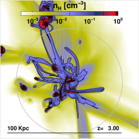
(a)

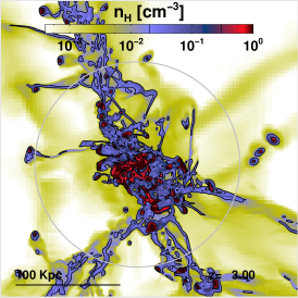
(b)

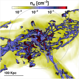
(c)

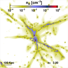
(d)

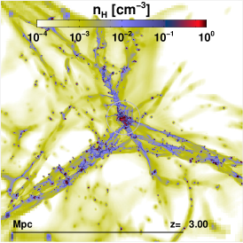
(e)

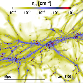
(f)

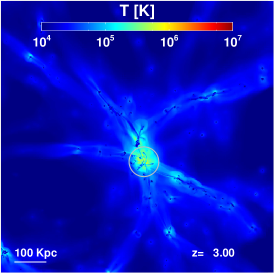
(g) H1

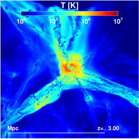
(h) H2

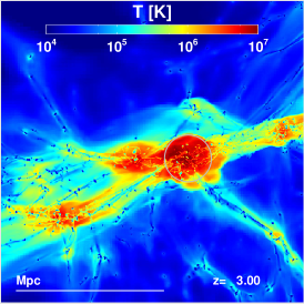
(i) H3

Figure 1: Redshift 3 maps of the three targeted halos in simulations H1, H2 and H3 from left to right (increasing halo mass). Grey circles indicate virial radii of the halos; $46$, $98$ and $158$ kpc for the H1, H2 and H3 halos respectively. Top row: Number density maxima along the line of sight, with contours marking $0.02$ and $0.3$ ${\rm{cm}}^{-3}$ as indicated in the color bars, corresponding to our definition of streams. Middle row: The same but zoomed out to show the large-scale environment. Bottom row: Mass weighted temperature maps, on the same scale as the middle row.

Operator splitting is a widely-used method of decomposing unwieldy differential equations into separate parts that can be solved independently and in sequence (e.g. Toro, 1999; Press et al., 1992). RamsesRT employs this method to split the radiative-hydrodynamics equations into (i) advection of gas and photons between cells and (ii) chemical reactions within the cells (radiative cooling and photo-heating). The advection part is first solved and then cooling, using the advection result as the initial state and subcycling when needed. Gas normally exists in a competition between advective/gravitational heating and radiative cooling, where the temperature ‘adjusts’ to a value where these processes cancel each other out. However, when the cooling time is shorter than the advection time, operator splitting may artificially give cooling the upper hand, leading to a slight underestimate in the temperature. Normally this is no big deal, but considering how sensitive Ly$\alpha$ emissivity is to gas temperature (see Fig. 6), this can result in a severe underestimate of Ly$\alpha$ emissivity in the gas. We’ve verified that this is indeed the case in our simulations. To prevent this from affecting our results, we restart the simulations at $z=3$ with the global timestep reduced by orders of magnitude, to make sure it is everywhere shorter than the local cooling-time, and run until we reach convergence in Ly$\alpha$ luminosity (this takes a few-thousand fine-cell time-steps).

Cell merging: With the bookkeeping on ionization states, and due to the fact that cell de-refinement takes place just before outputs are written in Ramses, special care must be taken on cell merging. Applying the traditional method of giving a merged cell a children-averaged ionization state can sometimes result in a combination of temperature and ionized state which causes it to outshine whole galaxies in Ly$\alpha$ emissivity (see discussion in Sec. 4.1). To prevent this we enforce a photoionization equilibrium (PIE) ionization state to merged cells, assuming the children-averaged values of gas density, pressure, and UV flux.

3 Physical properties of 3 halos

In this section, we first review the qualitative properties of our three simulated halos, and define the different phases of the intra-halo gas. We then describe in detail the impact of self-shielding on the ionization and thermal states of cold streams, and discuss the validity of an approximate treatment of self-shielding introduced by FG10.

3.1 Basic halo properties

Gas density maps of the three targeted halos at redshift 3 are shown in Fig. 1, in close-ups of the halos and zoom-outs to show their environments. Also shown are zoom-out maps of temperature. The halos display a tendency with increasing mass towards more intense, complex and fragmented accretion, and larger and hotter domains of shock-heated intergalactic medium (IGM).

The least massive halo (H1, left) has narrow (down to $\sim 1$ kpc in diameter) and unperturbed accretion streams and tidal tails stretching from the central galaxy, which can be seen in red at the center of the halo, edge-on and slightly inclined from the horizontal. It is about to undergo a major merger with another halo five times less massive, situated just outside $R_{vir}$ and coming in from the north. Two parallel accretion streams bridge the merging halos. Another accretion stream extends towards a factor 100 smaller merging halo, also at the edge of $R_{vir}$, but towards the line of sight (LOS), seen as a moon-shaped clump to the south-west. To the south and south-east are two relatively thick and diffuse accretion streams and another one even more diffuse to the west. Other structures in the map are orbiting satellites and tidal tails.

The intermediate mass halo (H2, middle) is more a group of orbiting galaxies than a single galaxy. On the large scale there is a network of filaments mixed with galaxies of varying masses, with at least 6 large scale streams extending towards the central halo. Movies show that the accretion here is notably more spiral than around the H1 halo, with the streams starting to curve around the center of gravity already well outside $R_{vir}$. Inside the halo we see plenty of streams and tidal tails, but much more disrupted and messy than in the H1 halo, as a result of stronger and more frequent interactions with other streams and galaxies.

This tendency continues with the most massive halo (H3, right), where we find even more disrupted streams, to the point that many of them seem to be completely obliterated close to the halo center. The H3 halo has just undergone a major merger, which makes the accretion activity particularly violent at this point in time.

To facilitate our analysis, we apply the following categorization to divide the gas into phases, as shown in the temperature-density phase diagram in Fig. 2 (note that the categorization is specific to this paper and does not apply in general):

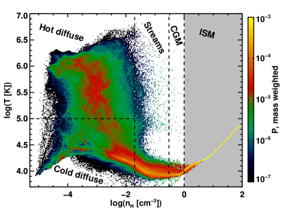
Figure 2: Phase diagram of the H1 halo, showing our density-dependent definitions of streams, CGM and ISM. The ISM is shaded to indicate that we always ignore ISM gas when adding up Ly$\alpha$ emissivities. The color scale represents mass weighted probability per temperature-density bin.

The star-forming ISM is all gas denser than $1$ ${\rm{cm}}^{-3}$ and as discussed in Sec. 2.2 we apply a temperature floor in the form of a density-dependent polytrope to keep this gas from artificially fragmenting, which manifests itself in the constrained temperature-density relation in the shaded area of the diagram. Our simulations lack the ingredients to accurately model Ly$\alpha$ emission from the ISM (multiphase resolution, dust, Ly$\alpha$ scattering) and our reaction to that is to simply ignore the Ly$\alpha$ emission from there in our analysis. The shaded color of the ISM region in Fig. 2 should remind the reader of this and that this work is about modelling the Ly$\alpha$ emission coming from galactic environments and not the galaxies themselves. The ISM gas density threshold is resolution dependent and reflects the density at which further collapse of gas – i.e. the Jeans length – is no longer resolved. At our chosen density threshold, assuming minimum temperatures of $10^{4}$ K, the Jeans length is resolved by approximately 10, 5, and 2.5 cell widths in the H1, H2 and H3 simulations respectively. It should be noted that our density threshold is almost an order of magnitude above what has typically been used in recent similar works (e.g. G10, FG10).

The CGM is gas with number densities between $0.3$ and $1$ ${\rm{cm}}^{-3}$. Ideally these densities form membrane interfaces between the ISM and their more diffuse environment. The lower density limit corresponds to the inner contours in the density maps of Fig. 1 (top row), and from those maps it can be seen that the CGM gas is indeed mostly constrained to galaxies (in red). In the phase diagram we find that most of the CGM gas is cooled down to the temperature floor of $\sim 10^{4}$ Kelvin where radiative cooling basically stops (metals can cool gas further but we don’t include those). Although CGM gas in our simulations is not directly affected by the polytropic equation of state, one may expect gas at densities $\ga 0.1\ {\rm{cm}}^{-3}$ to be multiphase and star-forming (Schaye, 2004). This cannot happen in our simulations because they don’t describe cooling below $\sim 10^{4}$ K, and this temperature floor provides artificial pressure support for dense gas. This implies a potentially high error in our predictions for the Ly$\alpha$ luminosities of halos, resulting from an overestimated CGM contribution. Thus, while we in general include the CGM gas in our analysis of Ly$\alpha$ luminosities, we also consider at some points the effect of excluding it, to get a grip on how sensitive our results are to the density thresholds applied. In summary we find that GCM gas typically provides a $~{}40\%$ of the Ly$\alpha$ luminosities of our simulated halos, but that in terms of Ly$\alpha$ extent it is less substantial.

Streams are defined in this work as gas with densities between $0.02$ and $0.3$ ${\rm{cm}}^{-3}$. These limits correspond to the density contours in Fig. 1 (top row) and from those we can see that these densities indeed correspond to thin filamentary structures. Much like the CGM most of the stream gas is found at the bottom of the temperature curve at $\sim 10^{4}$ K though we do see an increase in temperature in the more diffuse stream gas due to a combination of photo/gravitational heating and inefficient cooling (because of the low densities). Gas at sub-stream densities turns out to be negligible in terms of Ly$\alpha$ emissivity and thus not very important to our results so we crudely split what remains into two categories.

Table 2: Halo sizes and mass budgets (% of mass within $R_{vir}$).

Halo	$R_{vir}$	DM	Stars	Gas
				ISM	CGM	Streams	Hot
H1	46 kpc	82%	8%	10%
				73%	3%	8%	8%
H2	98 kpc	81%	7%	12%
				60%	9%	16%	13%
H3	158 kpc	82%	5%	13%
				58%	6%	12%	23%

()

()

()

()

()

()

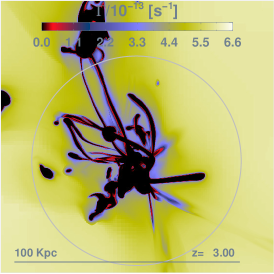
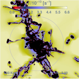
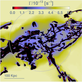
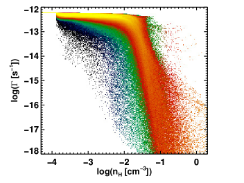
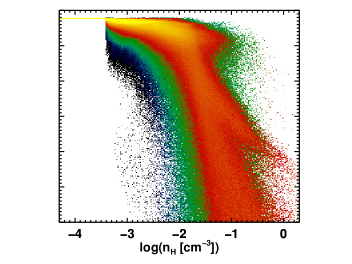
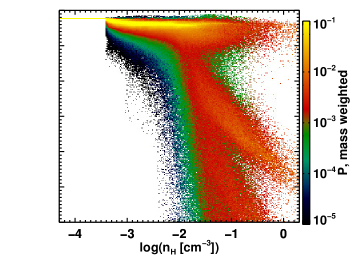
Figure 3: Self-shielding at redshift 3 in the three halos, from left to right, H1, H2 and H3. Top row: Maps of projected minima along the LOS of the hydrogen photoionization rate. The scale is non-logarithmic and in units of $10^{-13}\;\mathrm{s^{-1}}$. Bottom row: Phase diagrams of hydrogen photoionization rate versus density. The color scale represents mass-weighted probability per $\Gamma-n_{\rm{H}}$ bin over the plotted $\Gamma$ range.

Hot diffuse gas has been shock heated above $10^{5}$ Kelvin. As seen in the temperature maps in Fig. 1 (bottom row) this gas exists in abundance within the virial radii of the halos, but there also seems to be weaker heating around the large-scale accretion streams (and actually not so weak in the large streams around the H3 halo). Shock heating gets decidedly stronger with increasing halo mass, with gas reaching $\sim 2\ 10^{7}$ K in H2 and $\sim 6\ 10^{7}$ K in H3. Also, increasingly dense gas exists above $10^{5}$ K in the more massive halos; CGM in H2 and ISM in H3.

Cold diffuse gas is partly gas which is slowly condensing towards the streams and the CGM and partly cosmological gas that has not interacted with the halos at all and is being cooled down by the cosmological expansion.

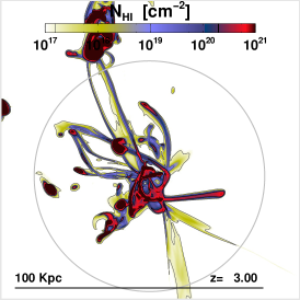
(a)

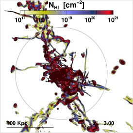
(b)

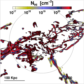
(c)

()

()

()

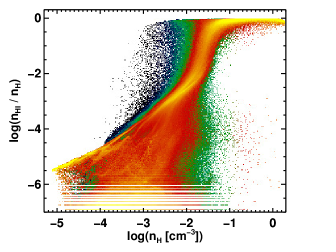
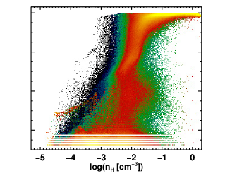
Figure 4: Neutral hydrogen at redshift 3 (H1, H2, H3 halos from left to right). Top row: Maps of projected Hi column density. Contours correspond to the lower limits for DLAs ($N_{\rm{H}}=2\ 10^{20}\;\mathrm{cm^{-2}}$), SLLSs ($10^{19}\;\mathrm{cm^{-2}}$) and LLSs ($1.6\ 10^{17}\;\mathrm{cm^{-2}}$). Bottom row: Phase diagrams of neutral hydrogen fraction, $x_{\rm{H\scriptscriptstyle I}}\equiv n_{\rm{H\scriptscriptstyle I}}/n_{\rm{H}}$, versus density. The color scale represents mass-weighted probability per $x_{\rm{H\scriptscriptstyle I}}-n_{\rm{H}}$ bin over the plotted $x_{\rm{H\scriptscriptstyle I}}$ range. The quantization-like horizontal lines at the bottom of all diagrams are due to numerical precision of the cell variable $x_{\rm{H\scriptscriptstyle II}}$ in RamsesRT, which is roughly seven digits.

The sizes and mass budgets of our three targeted halos are listed in Table  2. Each of the halo masses consists of roughly $80\%$ dark matter and $20\%$ baryons. The stellar/gas ratio decreases with halo mass, going from roughly one-to-one in H1 to about a one-to-three in H3. The gas mass is primarily in the ISM, going from $73\%$ in H1 to $58\%$ in H3. The hot gas fraction clearly increases with halo mass, going from $8\%$ in H1 to $23\%$ in H3 and correspondingly the cold fraction decreases, going from $8\%$ to less than $1\%$. Interestingly the stream fraction peaks in the intermediate mass halo at $16\%$, with half and two-thirds of that in H1 and H3 respectively. The low fraction in H1 can be explained by the smooth accretion that efficiently moves the gas straight into the ISM (hence a high ISM fraction), whereas H3 streams are disrupted to the point of obliteration when they approach the halo center (hence the low ISM fraction and large fraction of hot gas).

3.2 On-the-fly self-shielding

The transfer of UV photons gives us the opportunity to study the extent of self-shielding in gas clumps and streams. We quantify the local UV field intensity in terms of the hydrogen photoionization rate $\Gamma$, which expresses the average number of photoionization events per hydrogen atom per unit time (see Appendix B). In the UV model we use, the unattenuated photoionization rate at redshift 3 is $\Gamma=6.1\ 10^{-13}\;\mathrm{s^{-1}}$ (see Fig. 19), and shielded regions should have $\Gamma\rightarrow 0\;\mathrm{s^{-1}}$.

Fig. 3 shows the UV attenuation in the three targeted halos at redshift 3. The top row contains non-logarithmic maps of projected minima of the photoionization rate along the LOS. The light color on the edges of the maps corresponds to the unattenuated value. Towards the centers of the halos the UV field becomes increasingly attenuated due to photo-absorption of the gas and in the densest streams and clumps we see $\sim 100\%$ attenuation. The diffuse streams, with densities $\la 0.02$ ${\rm{cm}}^{-3}$, are not self-shielded. Gas at the centers of the H1 and H2 halos is efficiently shielded but at the center of the H3 halo gas is thermally ionized and thus optically thin.

The bottom row of Fig. 3 shows logarithmic phase diagrams of the hydrogen photoionization rate $\Gamma$ versus density for the same three halos. The most diffuse gas is UV emitting and has corresponding horizontal lines in the diagrams up to the $n_{H}^{UV}$-threshold. Above this threshold there is an immediate spread in the photoionization rate in all three halos, ranging from unattenuated UV to about half attenuated. Gas in the H1 halo is mostly self-shielded at $n_{H}\ga 2\ 10^{-2}$ ${\rm{cm}}^{-3}$. In more massive halos, the advent of thermal ionization in dense gas makes the situation more complex, and gas at $n_{H}\ga 2\ 10^{-2}$ ${\rm{cm}}^{-3}$ exists in two phases, either self-shielded as in H1 or optically thin. The bifurcation in the diagram around $\Gamma\sim 10^{-17}-10^{-15}\;\mathrm{s^{-1}}$, $n_{H}\sim 0.1-1$ ${\rm{cm}}^{-3}$, which grows more conspicuous with increasing halo mass is an effect of the ionization fronts becoming under-resolved at high densities, where the mean free path becomes comparable or shorter than the cell sizes. This feature does not affect our results.

Fig. 4 shows maps of Hi column densities and phase diagrams of neutral fraction $x_{\rm{H\scriptscriptstyle I}}\equiv n_{\rm{H\scriptscriptstyle I}}/n_{\rm{H}}$ vs. density. We find the CGM and ISM regions correspond mostly to damped Ly$\alpha$ absorbers (DLAs, $N_{\rm{H}}>2\ 10^{20}\;\mathrm{cm^{-2}}$) and the streams to Lyman limit systems (LLSs, $N_{\rm{H}}=1.6\ 10^{17}-10^{19}\;\mathrm{cm^{-2}}$) and even super Lyman limit systems (SLLSs, $N_{\rm{H}}=10^{19}-2\ 10^{20}\;\mathrm{cm^{-2}}$), according to the definitions found in e.g. Fumagalli et al. (2011). The column densities are likely over-estimated where they are highest due to lack of locally enhanced UV from star-formation. We see in the phase diagrams an abrupt transition of cold gas from ionized to neutral states, at about $5\ 10^{-2}$ ${\rm{cm}}^{-3}$ in all halos. This generic result is consistent with early expectations from Schaye (2001) and recent numerical estimates (e.g. Kollmeier et al., 2010; Faucher-Giguère et al., 2010; Aubert & Teyssier, 2010). The dense ($n_{H}\sim 0.1$ ${\rm{cm}}^{-3}$) and ionized ($x_{\rm{H\scriptscriptstyle I}}\la 10^{-4}$) cells which become increasingly abundant with halo mass correspond to hot shock-heated gas, which is thermally ionized and optically thin.

3.3 A self-shielding approximation

Figure 5: Phase diagram of neutral fraction versus density at redshift 3, in a version of the H1 simulation where a self-shielding approximation is used (instead of RHD) of applying full-strength UV background at densities below $10^{-2}$ ${\rm{cm}}^{-3}$ and zero strength above.

FG10 applied a self-shielding approximation in their simulations, where a UV field is applied homogeneously to gas but with a cutoff at an assumed self-shielding density threshold of $10^{-2}$ ${\rm{cm}}^{-3}$. We have run an analogue to our H1 simulation using the same self-shielding approximation instead of radiative transfer. Fig. 5 shows the neutral fraction versus density phase diagram at $z=3$ in this simulation. Apart from a much more discrete jump from ionized to neutral, the diagram is similar to the RHD counterpart (Fig. 4, bottom left), and we find $50\%$ neutral fraction at half the density of the RHD counterpart, or at $0.025$ ${\rm{cm}}^{-3}$. In terms of getting right the ionization state of gas at redshift 3 it thus appears that this non-RT self-shielding approximation holds fairly well. One might perhaps consider moving the self-shielding threshold a factor of two towards higher density, but one should be careful not to move it higher than that to avoid over-predicting Ly$\alpha$ emissivities due to photo-heating and photo-fluorescence. The approximation inaccurately describes UV attenuation in more massive halos, where much of the gas is thermally ionized and thus UV transparent. This doesn’t matter however, since an absence/presence of the UV background in gas which is already so ionized has a negligible effect on its Ly$\alpha$ emissivity (which is dictated by collisional ionization equilibrium (CIE) heating/cooling.

4 Predicted Ly$\alpha$ luminosities

4.1 Computing the gas Ly$\alpha$ emission

In most astrophysical contexts, an electron in the excited level 2P of the hydrogen atom will practically instantly relax to the ground state (1S) via the emission of a Ly$\alpha$ photon. There are two channels to produce such excited atoms, and hence to produce Ly$\alpha$ radiation:

Collisional: A collision with a free electron excites the H-atom, which may release a Ly$\alpha$ photon when it relaxes back to the ground state. The collisional emissivity is approximated with

$$\varepsilon_{coll}=C_{{\rm{Ly}\alpha}}(T)\;n_{\rm{e}}\;n_{\rm{H\scriptscriptstyle I}}\;\epsilon_{{\rm{Ly}\alpha}},$$ (4)

where $n_{\rm{e}}$ and $n_{\rm{H\scriptscriptstyle I}}$ are number densities of electrons and neutral hydrogen, respectively, and $C_{{\rm{Ly}\alpha}}(T)$ is the rate of collisionally induced 1S-to-2P level transitions. An expression for this rate is given by G10, fitting results from Callaway et al. (1987). It is always less than the hydrogen collisional excitation cooling rate, $\Lambda_{coll}^{HI}$, used in the code (from Maselli et al., 2003), since cooling also takes into account excitations to atomic states other than 2P (the most likely of which is the non-Ly$\alpha$ releasing 2S state). The ratio of $C_{{\rm{Ly}\alpha}}/\Lambda_{coll}^{HI}$ goes from $71\%$ at $10^{4}$ K to $57\%$ at $5\ 10^{4}$ K.

Recombinative: A free electron combines with a proton at any level ($\geq 2$), and may cascade down to the 2P level. The recombinative Ly$\alpha$ emissivity of this process is given by

$$\varepsilon_{rec}=0.68\;\alpha^{\rm{B}}_{\rm{H\scriptscriptstyle I}}(T)\;n_{\rm{e}}\;n_{\rm{H\scriptscriptstyle II}}\;\epsilon_{{\rm{Ly}\alpha}},$$ (5)

where the $0.68$-factor is the average number of Ly$\alpha$ photons produced per case B recombination (from Osterbrock & Ferland, 2006) and $\alpha^{\rm{B}}_{\rm{H\scriptscriptstyle I}}(T)$ is the case B recombinations rate, i.e. counting recombinations to all levels except directly to the ground one. We use the expression from Hui & Gnedin (1997).

Unless otherwise specified, the Ly$\alpha$ emissivities calculated in this paper are:

$$\varepsilon=\varepsilon_{coll}+\varepsilon_{rec}.$$ (6)

Figure 6 shows the collisional and recombinative Ly$\alpha$ emissivities of gas at typical stream density, assuming the gas is UV exposed (thick curves) and self-shielded (thin). Also shown in dotted black curves is the neutral fraction of the gas, approximately extracted using a simplified model of hydrogen-only and PIE/CIE equilibrium.

The plot illustrates that it is crucial to be consistent in following the gas state of $(T,x_{\rm{H\scriptscriptstyle I}},\Gamma)$ in the simulation code, since independently changing one of those factors without considering the effect on the others can have a dramatic effect on $\varepsilon$. If, for example, self-shielding is assumed in post-processing and the neutral fraction changed accordingly without considering the change in temperature, the $\varepsilon_{coll}$ estimate can increase by almost an order of magnitude. This is unphysical – what really happens if gas suddenly becomes UV shielded is that the temperature drops somewhat due to lack of photo-heating, the end-result being a slightly lowered value of $\varepsilon$.

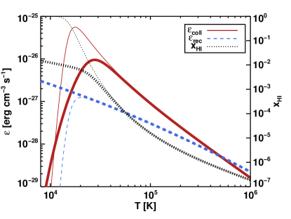
Figure 6: Ly$\alpha$ emissivity of gas at number density $n_{\rm{H}}=3\ 10^{-2}\;{\rm{cm}}^{-3}$, which is close to the lower limit for accretion streams in our simulations. Thick curves show gas exposed to a UV field with $\Gamma=6.1\ 10^{-13}\;\rm{s}^{-1}$, corresponding to redshift 3. Thin curves show UV shielded gas ($\Gamma=0\;s^{-1}$). Blue dashed curves show recombinative Ly$\alpha$ emissivity, red solid curves show collisional Ly$\alpha$ emissivity and black dotted curves show the approximate neutral hydrogen fraction in the gas, assuming equilibrium between photoionization, collisional ionization and recombinations.

The accuracy of the $(T,x_{\rm{H\scriptscriptstyle I}},\Gamma)$-state is secondary to consistency, because if the code handles things properly, $\varepsilon$ should simply reflect the work put into the gas by the UV background and gas advection. In the limit that the UV energy input is negligible compared to gravitational heating, accurate modelling of the UV background isn’t really crucial in the context of Ly$\alpha$ emissivity, and applying e.g. a sensible shielding approximation like the one discussed in Sec. 3.3 should be OK. This breaks down when UV photo-fluorescence becomes non-negligible.

4.2 Intrinsic luminosities

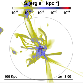
(a)

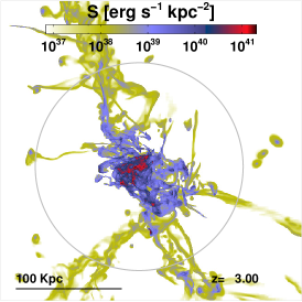
(b)

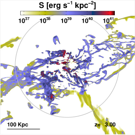
(c)

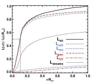
(d)

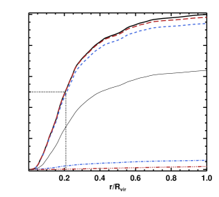
(e)

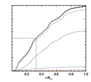
(f)

Figure 7: Top row: Rest-frame Ly$\alpha$ surface brightness maps of the targeted halos (H1, H2 and H3 simulations, from left to right). Bottom row: Radially (3D) cumulative Ly$\alpha$ luminosities of the same halos. The thick black curves show the total luminosity. The dotted lines denote at what radius $50\%$ of the total luminosity is accounted for. The blue curves show how the total luminosity is split between collisional and recombinative channels, given in Eqs. 4 and 5 respectively. The red curves show how the total is split between the contributions of the UV background and gravitational dissipation, discussed in Sec. 5.2. The thin black curves show the contribution of sub-CGM density gas (i.e. mostly streams) to the total luminosities.

Fig. 7, top row, shows maps of the rest-frame Ly$\alpha$ surface brightness $S$ of the three targeted halos, which is calculated by integrating the Ly$\alpha$ emissivity (Eq. 6) along the LOS. We don’t take absorption or scattering into account: These factors would certainly diminish the brightest spots associated with CGM regions, but we don’t expect them to affect the more diffuse streams much (see discussion in Sec. 4.3). The surface brightness is concentrated around CGM regions in all three halos, with $S\approx 10^{40}-10^{41}\;{\rm{erg\,s^{-1}\,kpc^{-2}}}$, and the brightness in streams is typically lower by one or two orders of magnitude.

The bottom row in Fig. 7 shows radially cumulative Ly$\alpha$ luminosities for the halos, i.e. fraction of the total luminosity within a given radius (black solid curves). Streams and the diffuse medium consistently contribute about 60% of the total luminosity, as indicated by the thin black curves.

It is evident from both the maps and plots that there is a trend of more extended emission with increasing halo mass. In the H1 halo, half of the total luminosity comes from the central $16\%$ of the virial radius (dotted lines), while in H2 this radius is $20\%$ and $33\%$ in H3. Partly this is because the more massive halos consist of increasing quantities of orbiting galaxies so the surface brightness is just following the increased spread of CGM regions, as can be seen from red dots of surface emissivity in the maps and from corresponding steps in cumulative surface brightness in the plots. That is not the whole story though: The streams become more efficient Ly$\alpha$ emitters with increasing halo mass.

As seen from the blue curves in the luminosity plots, electron-hydrogen collisions dominate the total luminosity, and recombinations are borderline negligible, as should be expected outside ISM regions. This dominance increases with halo mass, with recombinations contributing $10\%$ to the total in the H1 halo and only about $5\%$ in H2 and H3. The red curves in Fig. 7 will be discussed in Sec. 5.

In Fig. 8 we plot total halo luminosities versus halo mass (which is defined, as in Table  1, as the total mass of all dark matter and baryons within the virial radius). From each of the three simulations we extract all halos from within the zoom-in volume and integrate Eq. 6 over their virial radii, excluding ISM gas. The halos roughly line up into a power law indicated by a red solid line, with exponent $1.25$. There is a systematic tendency for halos in more massive simulations to be more luminous for a given mass, which is presumably an environment effect since the cosmological over-density of the zoom-in regions increases between the H1, H2 and H3 simulations respectively.

Large thick symbols mark the three main halos targeted in our simulations. For those we also plot luminosities excluding consecutive phases of gas. Blue symbols show luminosities when ignoring the ISM and the CGM, and green symbols show what happens if we also ignore the stream densities. The CGM accounts for about 40% of the total luminosity in all three targeted halos (see also Fig. 7) and the streams account for most of the rest, or $50-60\%$, with sub-stream densities accounting for $8\%$, $4\%$ and $2\%$ in the targeted halos of H1, H2 and H3 respectively.

As can be read directly from Eqs. (4) and (5), the Ly$\alpha$ emissivity of gas in principle scales with density squared, though temperature and ionization state have their influence as well. Fig. 9 shows a luminosity weighted phase diagram of Ly$\alpha$ emissivity of gas versus density in the H1 halo (the H2 and H3 diagrams are similar). Over-plotted on the diagram in dashed grey lines are two power laws that the gas emissivity approximately follows, with a knee between $10^{-2}$ and $10^{-1}$ ${\rm{cm}}^{-3}$. The knee roughly corresponds to where the gas becomes self-shielding and the change in slope is caused by the corresponding transition in temperature and ionization state. Below the knee the gas emissivity is split in two ridges with slightly different slopes. The upper one has power index $\approx 2.5$ and is dominated by collisional emission (Eq. 4), whereas the lower one has power index $\approx 2.2$ and is dominated by recombinations (Eq. 5). The emissivity above the knee is completely dominated by collisions. The stronger than $2$ power law below the knee stems from the increasing abundance of neutral atoms with density and a temperature that tends towards peak Ly$\alpha$ emissivity, whereas the less than $2$ power law above it results from the decreasing relative abundance of electrons with density.

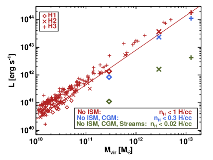
Figure 8: Total halo luminosities versus halo mass for the three simulations. The halos are extracted from the zoom-in volumes, and we exclude sub-halos. The three targeted halos are indicated by large thick symbols. For those halos we also show luminosities excluding different phases of the gas. The red solid line indicates a power-law with exponent $1.25$.

4.3 Observational properties

We now consider mock observations of our simulated halos. To produce those we first convert the rest-frame surface brightness maps in Fig. 7 to observed surface brightness $I$, using

$$I=\frac{S{f_{\alpha}}}{4\pi(1+z)^{4}},$$ (7)

where ${f_{\alpha}}$ is a cosmological transmission factor that accounts for absorption and scattering of Ly$\alpha$ photons on the LOS from the object to the observer. We adopt in this paper a value of ${f_{\alpha}}=0.66$ based on the work of Faucher-Giguère et al. (2008). (${f_{\alpha}}$ is only applied to mock observations and not to the intrinsic emissivity and luminosity, Figures 7 and 8). To the result of Eq. 7, we then apply a Gaussian point spread function (PSF) with a $0.6$ arcsec full width at half maximum (FWHM) to mimic atmospheric and instrumental distortion, and assume a camera pixel size of $0.2$ arcsec (Fig. 10). This corresponds to very good seeing conditions in state-of-the-art instruments. We present maps made with a PSF about twice as broad in Appendix C. These are directly comparable to the observations of M11.

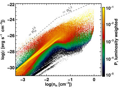
Figure 9: Phase diagram showing Ly$\alpha$ emissivity of gas versus density at z=3 in the H1 halo. Each density bin is Ly$\alpha$ luminosity weighted independently. The grey dashed lines show power laws that approximately fit the data. The color scale represents Ly$\alpha$ luminosity weighted probability per $\varepsilon-n_{\rm{H}}$ bin over the plotted $\varepsilon$ range.

Unlike FG10, we don’t model the scattering of Ly$\alpha$ photons in this work. These authors show that Ly$\alpha$ transfer dominates the spectral shape of extended Ly$\alpha$ emission, but hint that it has little effect on the morphology and extent. Their Fig. 8 shows this to be the case for a halo corresponding in mass to our H1 halo, if only the Ly$\alpha$ emissivity of gas is considered – though their Fig. 9 also illustrates that strong point-like sources can produce extended Ly$\alpha$ structures via scattering. We will assume here that scattering has little overall effect on our predicted morphologies and extents, in the case that these structures are already well extended, though we do expect that it will likely produce subtle changes in observable LAB areas – indeed Fig. 8 in FG10 shows that the inclusion of scattering can make some observable Ly$\alpha$ structures narrow down and others widen out. We will include and investigate the effect of Ly$\alpha$ scattering on spectral shapes, luminosities, and morphologies of our objects in a future paper.

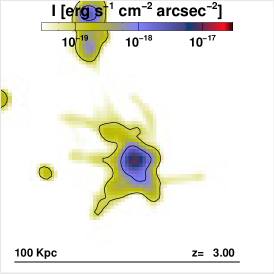
(a)

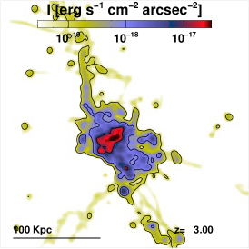
(b)

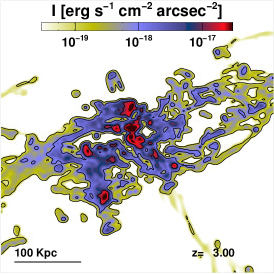
(c)

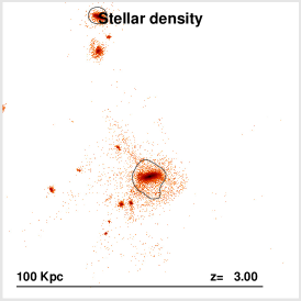
(d)

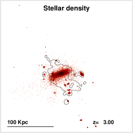
(e)

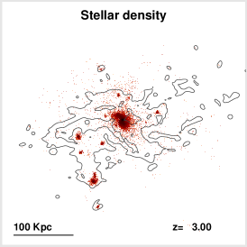
(f)

Figure 10: Top row: Mock images showing predicted observed surface brightness in the targeted halos of H1, H2 and H3, from left to right. The contours mark $10^{-17}$, $10^{-18}$ and $10^{-19}$ $\mathrm{erg\,s^{-1}\,cm^{-2}\,arcsec^{-2}}$. The images where computed using an optimistic PSF of FWHM 0.6 arcsec. Bottom row: Stellar density maps for the same halos, illustrating that the bright spots of Ly$\alpha$ emission are centered on galaxies. Over-plotted are contours marking $10^{-18}\,\mathrm{erg\,s^{-1}\,cm^{-2}\,arcsec^{-2}}$ in observed surface brightness (the middle contours from the upper maps).

4.3.1 Observed blobiness of cold accretion streams

Mock observations of our three targeted halos are shown in the top row of Fig. 10. The middle contour in the maps is set at $I_{-18}=10^{-18}\;{\rm{erg\,s^{-1}\,cm^{-2}\,arcsec^{-2}}}$, roughly corresponding to current observation limits (e.g. M11, Erb et al., 2011, see Appendix C for a more accurate comparison), and the inner and outer contours correspond to ten times brighter and ten times dimmer, i.e. $10^{-17}$ and $10^{-19}\;{\rm{erg\,s^{-1}\,cm^{-2}\,arcsec^{-2}}}$.

Assuming $I_{-18}$ as our instrumental sensitivity limit, the H1 halo (top left) is a Ly$\alpha$ emitter that is centered on a galaxy, circularly symmetric in shape, about $20$ kpc in diameter and doesn’t trace streams. Thus the H1 halo is not a LAB. The total observed luminosity, i.e. $I$ integrated over the area within $I_{-18}$, is $L_{obs}=6\ 10^{41}$ $\mathrm{erg\,s^{-1}}$.

The H2 halo observation (top middle) differs dramatically from that of H1. At $I_{-18}$ we do see a borderline giant LAB, asymmetric and about $100$ kpc in length, and we can see the end of an accretion stream poking out to the north-west. The observed luminosity integrated above $I_{-18}$ is $L_{obs}=2\ 10^{43}$ $\mathrm{erg\,s^{-1}}$. The H3 halo (top right) has observable Ly$\alpha$ emission all over the place, is about $200$ kpc in diameter and very asymmetric. Its observable luminosity is $L_{obs}=10^{44}$ $\mathrm{erg\,s^{-1}}$.

Provided there is nothing special about these halos, we can conclude that in general the cooling emission from halos with masses greater than a few times $10^{12}\,\mathrm{M_{\sun}}$ can produce giant LABs ($\ga 100$ kpc) at redshift 3, assuming current instrument sensitivity limits. Qualitatively this compares well with Yang et al. (2010), who find that at redshift 2.3, LABs should occupy halos $\ga 10^{13}\,\mathrm{M_{\sun}}$. Qualitatively again, the maps presented in Sec. C, which mimic the observational conditions of M11, show that the morphologies of our simulated LABs are very similar to those observed.

Interestingly, we note that the LABs produced by cold accretion streams are naturally extended in the direction of the main large-scale filaments that they are connected to. This is particularly visible for H2 and H3 in Fig. 10 (see also Fig. 14), and lends support to the observational findings of Erb et al. (2011).

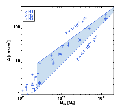
Figure 11: Plot of mock observed areas within contours of $1.4\ 10^{-18}\;{\rm{erg\,s^{-1}\,cm^{-2}\,arcsec^{-2}}}$ versus halo mass for zoomed halos in the three simulations. Each halo is observed from three directions. The targeted halos are marked with thick symbols. The points are enveloped by two power-laws shown in the plot.

Another matter are those mysterious LABs which do not seem to be centered on observed galactic counterparts (e.g. Steidel et al., 2000; Weijmans et al., 2010; Prescott et al., 2011). We are not able to reproduce this phenomenon in our simulations. The bottom row of Fig. 10 shows stellar densities in our targeted halos, with the $I_{-18}$ sensitivity contour over-plotted. Clearly all the peaks of Ly$\alpha$ brightness would have continuum counterparts in observations, unless these counterparts would for some reason be hidden from view. Such LABs are rare among rare events, though, and our three simulations have little statistical chance of reproducing such oddities. A larger sample of simulations would be required to investigate this issue further.

4.3.2 Size distribution of simulated LABs

We shall now statistically compare our results with a catalogue of 202 observed LABs from the surveys described in M11 (courtesy of Yuichi Matsuda and team). The aim here is to derive a cumulative LAB area function from our results and see how it compares with real data.

We follow M11 by assuming $z=3.1$ in Eq. 7, and applying a PSF with FWHM=1.4 arcsec. We calculate the observed LAB area $A$ of each halo within the zoom regions of our simulations by integrating its total area above the surface brightness limit $I=1.4\ 10^{-18}\;{\rm{erg\,s^{-1}\,cm^{-2}\,arcsec^{-2}}}$. We ‘observe’ each halo in three directions ($x$, $y$, and $z$). In Fig. 11, we plot the LAB areas as a function of halo mass. The large thick symbols correspond to our targeted halos H1, H2, and H3. The observed LAB area is a reasonably well-behaved function of halo mass, with more massive halos producing larger LABs, and the points can be bracketed by a couple of power laws of indexes 0.87 and 1.19 (see Fig. 11).

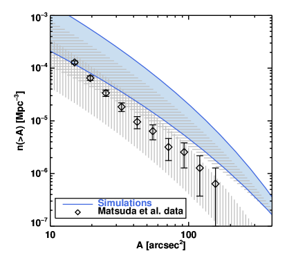
Figure 12: The shaded region represents the boundaries of our predicted LAB area function, derived from the power laws in Fig. 11. The black symbols mark a rough area function derived from a sample of 202 observed LABs from the survey of M11. The horizontally and vertically line-filled regions represent similarly predicted area functions, but with gas densities of $n_{\rm{H}}\geq 0.3$ ${\rm{cm}}^{-3}$ and $n_{\rm{H}}\geq 0.1$ ${\rm{cm}}^{-3}$ excluded, respectively.

We now make the assumption that extended Ly$\alpha$ emission is an inherent property of dark matter halos and that the observed LAB properties are direct functions of halo mass. This assumption is substantiated by our results (Figs. 8 and 11). We thus convolve the power laws of Fig. 11 with the halo mass function at redshift $3.1$ (taken from Sheth & Tormen, 1999) in order to produce the cumulative area function envelope shown in Fig. 12. There, the black diamonds represent actual observations for comparison: they are a rough estimate of the area function at redshift 3.1 based on the 202 LABs of the M11 survey, derived by binning the LABs by area and dividing the count by the total survey volume of $1.57\ 10^{6}$ Mpc³ (the error bars are Poissonian). The comparison between our predicted area function and the observationally derived one is very satisfactory, although we systematically over-predict the function by a factor of 2-3.

There may be several causes to this over-prediction. First, our derivation of the observed LAB area function is too simplified. For example, we do not take into account the shape of the narrow band filter, or any $1/V_{\rm max}$ corrections. This introduces systematic errors that could well be of about a factor two. Second, our mock observations are also simplified, and do not include noise, which could possibly affect the measured area in a systematic way. Third, perhaps we have overshot in our choice of ${f_{\alpha}}=0.66$. As noted by G10, cosmic extinction may be stronger than average for sources that reside in over-dense regions, as LABs tend to do. Fourth, our prediction is based on only a few objects and to a lesser degree the same applies to the observation-derived function. Fifth, the predicted LAB areas are sensitive to the applied PSF smoothing, which may not be entirely consistent in all the 202 observed LABs. And finally, we may lack physics in our simulations that would drive down the LAB areas. For example, Ly$\alpha$ scattering, if applied, could induce a slight spread in the predicted rest-frame Ly$\alpha$ surface brightness, which could in some cases bring down both the observed area and luminosity within sensitivity ordained brightness contours. Also, metal-line cooling may drive down the Ly$\alpha$ emissivity of gas by cooling it below $10^{4}$ K. Furthermore, as shown by van de Voort et al. (2011b), Faucher-Giguère et al. (2011), and van de Voort & Schaye (2011), feedback driven winds can destroy cold accretion streams in the vicinity of galaxies, hence terminating their Ly$\alpha$ emissivities.

Our predicted area function is not very sensitive to the density threshold of gas applied throughout this paper, where we have excluded ISM densities ($n_{\rm{H}}>1$ ${\rm{cm}}^{-3}$) in our analysis. To illustrate this, Fig. 12 also shows, with line filled regions, predicted area function envelopes that have been derived from our simulations via a convolution with the Sheth-Thormen halo mass function, but including only more diffuse gas, $n_{\rm{H}}<0.3$ ${\rm{cm}}^{-3}$ (i.e. sub CGM densities) and $n_{\rm{H}}<0.1$ ${\rm{cm}}^{-3}$, for the horizontal and vertical line-fillings respectively. The prediction using the sub-CGM densities is close to the original prediction, which can be expected since these densities account for $\sim 60\%$ of the total luminosities of all three targeted halos (see Figs. 7 and 8). Even using $n_{\rm{H}}<0.1$ ${\rm{cm}}^{-3}$ gas only (which is comparable to the more conservative prescriptions used in FG10) still produces giant LABs hosted by massive halos and gives an area function that is compatible to the observational data. This confirms that the extent of our simulated LABs is largely driven by low density cold streams.

We have also compared our results to observations via a LAB luminosity function (rather than the area function just discussed). However, since LAB emissivity typically peaks around compact sources, and since we neither model the emission nor absorption coming from the compact ISM regions, such a comparison is less robust than using the area function which should be more or less dictated by the state of more diffuse gas on much larger scales. The luminosity comparison, which is discussed in detail in Appendix D, is actually surprisingly good, but it is problematic to draw any conclusions from it because of the lack of modelling of compact regions.

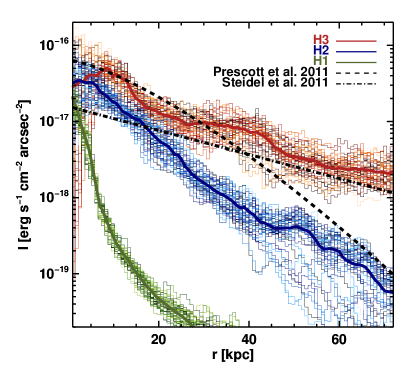
Figure 13: Surface brightness profiles of our three targeted halos (solid) compared to the profile of LABd05 from Prescott et al. (2011) (dashed) and an average surface brightness profile of 11 LABs from Steidel et al. (2011) (dot-dashed). The thin solid lines represent different random orientations (50 for each halo) and the thick solid ones are averages of the thin ones.

4.3.3 Surface brightness profiles

Fig. 13 shows observed surface brightness profiles of our three targeted halos. Profiles are taken for each halo in 50 planes of random orientation, represented by thin coloured lines, and then these are averaged into the thick coloured lines. The profiles are transformed from rest-frame to observed surface brightness via Eq. 7, assuming redshift 3, but no smoothing or cosmic extinction is applied, and as before Ly$\alpha$ scattering is neglected. Over-plotted are surface brightness profiles from observations: The black dashed curve represents a Sersic fit to the observed profile of the giant LABd05 at redshift $2.656$ from Prescott et al. (2011), which we have scaled to z=3. Notably, LABd05 doesn’t have a galactic counterpart at, or even close to the peak of Ly$\alpha$ emission, though it has 17 small galaxies substantially offset from the peak (by $\ga 20$ kpc). The black dot-dashed curve is an exponential disk fit to an average of 11 LAB profiles observed at $z\approx 2-3$, reported in Steidel et al. (2011), with no scaling applied.

The profiles of H2 and H3 are similar in shape and magnitude to the observed profiles. Interestingly, each of those compares favourably to different observations, with the H2 profile being similar to LABd05 and the H3 profile similar to the 11 LABs from Steidel et al. (2011). The comparison indicates that these observations fit well within the model of cold accretion powered LABs, but due to the very limited statistics of our simulations (i.e. one halo per mass bin of three), and different redshifts of the observed LABs, it is problematic to make quantitative deductions, e.g. about masses of the host halos of observed LABs. Rather than representing different halo masses, the different profile shapes (and to some degree their magnitudes) may just as well reflect the different morphologies one may find in galactic groups and clusters.

Prescott et al. (2011) compare the LABd05 surface brightness profile with simulated profiles from G10 and FG10, and find that the simulations appear to fit very badly with reality, with the G10 profile being both too peaky at the center and too shallow at large radius, and the FG10 profile being too weak and steep. Our H1 profile actually agrees with the simulated profile from FG10 (their model 7, see Fig. 9 in Prescott et al. 2011), and it seems to us that FG10 in fact don’t pose any mismatch with the LABd05 observation: The fault lies in Prescott et al. (2011) assuming that the surface brightness profile scales linearly with halo mass, which is not at all the case judging from our simulations (and to be fair, these authors admit that their assumption is probably not accurate).

We admittedly don’t provide large statistics here, but we can conclude that the surface brightness profiles produced by our simulations do not disagree with LAB observations, and at the same time we can argue that neither do the simulations of FG10.

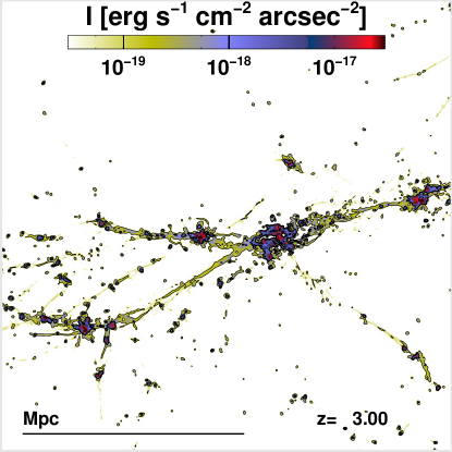
Figure 14: Same as Fig. 10, but showing the large-scale Ly$\alpha$ map of the H3 halo and its environment. Thick inner (thin outer) contours mark $I=10^{-18}\;(10^{-19})\,{\rm{erg\,s^{-1}\,cm^{-2}\,arcsec^{-2}}}$. Large-scale streams connecting massive halos and extending over several Mpc would be visible at $10^{-19}\,{\rm{erg\,s^{-1}\,cm^{-2}\,arcsec^{-2}}}$.

4.3.4 Implications for future observations

Having demonstrated reasonable agreement between our simulations and LAB observations, we now wish to highlight a prediction from our work which is particularly relevant in the context of direct searches for IGM emission at high redshifts. The outermost contours in the upper row of Fig. 10 mark Ly$\alpha$ brightness at $10^{-19}\;{\rm{erg\,s^{-1}\,cm^{-2}\,arcsec^{-2}}}$. At this limit, accretion streams start to show up even in the least massive halo, and in the more massive halos we would detect them unambiguously. The deepest observations to date are not quite there yet, but almost, and this is an exciting perspective. Perhaps even more exciting is the map shown on Fig. 14, where the thin (resp. thick) contours again mark the limit at $10^{-19}$ (resp. $10^{-18}$) ${\rm{erg\,s^{-1}\,cm^{-2}\,arcsec^{-2}}}$. This zoomed out view of our H3 halo shows that deep Ly$\alpha$ observations around massive halos may even reveal the large-scale filamentary structure of the IGM on scales of a few Mpc !

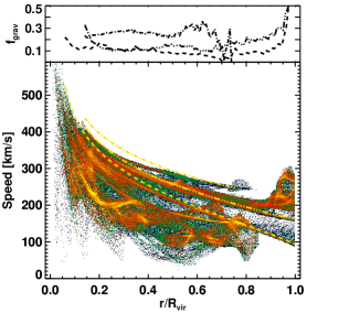
(a)

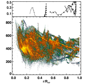
(b)

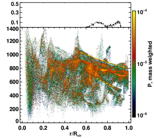
(c)

Figure 15: Phase diagrams showing speed of stream gas as a function of radius within targeted halos H1, H2 and H3 from left to right. The color scale represents mass weighted probability per speed-radius bin. Only stream densities are included here so that the streams stand out in the diagrams and are not drowned in the more diffuse gas. Over-plotted in yellow are free-falling speed profiles. Plots above each phase diagram show gravitational heating efficiency in the clearest streams, compared to the free-fall profiles.

Although such observations are extremely challenging (if not plain impossible) today, upcoming instruments, such as MUSE (Bacon et al., 2006) or K-CWI (Martin et al., 2010), should greatly increase our chances of observing directly this source term of galaxy formation in a very near future.

5 What drives the Ly$\alpha$ emission?

Since Ly$\alpha$ scattering and stellar feedback are not included in our simulations, the only possible power sources of Ly$\alpha$ emission in our results are gravity and the UV background. We now look at how gravitational heating contributes to the Ly$\alpha$ emission along streams and attempt to quantify its efficiency. We consider the contribution of UV fluorescence and show how it is sub-dominant for typical values of the UV background. We conclude this section by discussing to what extent locally enhanced UV fluxes could boost Ly$\alpha$ emission from cold streams.

5.1 Gravitational efficiency

Gravitational heating is generally viewed as a progressive release of gravitational potential energy that heats the gas along the cold streams (Dijkstra & Loeb, 2009). As long as this heating is not too fast it can be balanced by radiative cooling, and as long as the gas remains metal-poor and at temperatures $\sim 10^{4}$ K, Ly$\alpha$ emission is the dominant cooling mechanism, meaning that the thermal energy is efficiently converted into Ly$\alpha$ photons.

Gravitational heating in cold streams can be parametrized by the gravitational efficiency $f_{grav}$, the fraction of the change in gravitational potential that dissipates into thermal energy during in-fall. The rest is converted into bulk kinetic energy, increasing the speed of the gas. A value of $f_{grav}=1$ thus means perfect conversion of potential into heating, implying constant in-fall speed, and $f_{grav}=0$ means that there is no conversion into thermal energy and the stream should be in free-fall. Dijkstra & Loeb (2009) derive an analytic model in which $f_{grav}\ga 20\%$ is required if Ly$\alpha$ blobs are to be driven by gravitational heating in cool flows.

For each stream we can distinguish in our simulated halos in a given output, we can extract the stream speed profile $v_{str}(r)$ by following its core from end to end. Using this and a corresponding free-fall profile $v_{ff}(r)$ for a body starting at a position and speed identical to the outer end of the stream, we can estimate $f_{grav}$ with

$$f_{grav}(r)=\frac{v_{ff}^{2}(r)-v_{str}^{2}(r)}{v_{ff}^{2}(r)-v_{init}^{2}},$$ (8)

where $v_{init}$ is the speed at the outer starting position.

We calculate an approximate free-fall profile for the stream by assuming static state and spherical symmetry, integrating the free-fall speed from the starting position towards the halo center using

$$dv_{ff}(r)=\frac{1}{v_{ff}(r)}\frac{GM(<r)}{r^{2}}\;dr,$$ (9)

where $r$ is radius, $G$ is the gravitational constant and $M(<r)$ is the total halo mass within $r$.

In practice we divide the halo mass into radial bins $r_{i}$, where increasing $i$ corresponds to decreasing radius, and solve Eq. 9 by recursively computing

$$v_{ff}(r_{i+1})=v_{ff}(r_{i})+\frac{1}{v(r_{i})}\frac{GM(<r_{i+1})}{r_{i+1}^{2}}(r_{i+1}-r_{i}),$$ (10)

where $M(<r_{i+1})$ is the mass measured within $r_{i+1}$ in the simulation, and the initial condition is the stream speed at the outer end, $v_{ff}(r_{0})=v_{init}$.

In Fig. 15 we show phase diagrams for the three targeted halos of gas speed versus radius (normalized to $R_{vir}$), where we exclude all but gas at stream densities, so that the streams can stand out more clearly. In the smallest halo (H1) the streams pop out nicely, smooth and undisturbed basically over the whole radius range, though they do dilute a bit at the central 10% of $R_{vir}$. In H2 we can still see streams, but they are much more disrupted, and not distinguishable within the central 20% of $R_{vir}$. In H3 only a few streams can be distinguished in the outer $40\%$ of $R_{vir}$, and in the central $\sim 20\%$ they are completely destroyed.

For those streams we can clearly distinguish in the diagrams, we have plotted in yellow the corresponding free-fall profiles, using Eq. 10, which show approximately the speeds that the streams would follow were they in free-fall. Qualitatively it can be seen that the streams are close to free-fall, though usually they lag a little behind the free-fall profile, and conversely on some occasions we even see streams that seem to accelerate faster than free-fall (due to sub-halos and/or the inaccuracy of assuming static state and spherical symmetry in our free-fall calculation).

We plot our estimates of $f_{grav}$ using Eq. 8 directly above each phase diagram. For two of the three streams we have extracted in the H1 halo we get a fairly consistent estimate of $f_{grav}\sim 0.1$ from the halo outskirts towards the central $\sim 15\%$ of $R_{vir}$, whereas for the third (and more diffuse) stream we get a value which is two to three times higher. In the H2 halo things are much messier, and for those fragments of streams that we can extract we find a large scatter in $f_{grav}$, going from negative values to about $0.3$ (the initial large values are a numerical noise due to resolution in the phase-space). Finally, in the H3 halo, we can only extract two streams at the outer edges of the halo, one of them showing $f_{grav}\sim 0.1$ and the other accelerating faster than our free-fall approximation.

It appears that gravitational heating is inefficient if seen only as a smooth and steady process along unperturbed streams as in H1. However, heating and subsequent release of Ly$\alpha$ photons seems to be more efficient when it involves disrupted and wiggly streams. This also appears reasonable, since the gas at the core of a straight and unperturbed stream can flow virtually unopposed towards the central galaxy whereas if the streams are wiggly and disrupted there should be greater opposition from the surrounding hot and diffuse gas.

It remains to be seen how much photo-fluorescence from the UV background is contributing the Ly$\alpha$ emissivities compared to gravitational processes, both smooth and messy. Before comparing these factors we describe how they’re derived from the simulation output.

5.2 Computing the Ly$\alpha$ contributions

Since we store the photon flux in each cell we can easily keep track of the photo-heating and photoionization rates in the gas. If we assume that every photoionization leads to a recombination and that all the energy provided by photo-heating is released via collisional excitations, we can estimate the UV contribution to the Ly$\alpha$ emissivity in each cell as:

$$\varepsilon_{UV}=0.7\;\mathcal{H}_{\gamma}+0.68\;\Gamma\;n_{\rm{H\scriptscriptstyle I}}\;\epsilon_{{\rm{Ly}\alpha}},$$ (11)

where $\mathcal{H}_{\gamma}$ is the photo-heating rate, the $0.7$-factor is the conversion efficiency of cooling into Ly$\alpha$ photons, and the second term on the right is akin to Eq. 5. We refer to Appendix B for how to calculate the photo-heating rate. The UV contribution tends to be overestimated and can in fact be estimated higher than $\varepsilon$ in hot regions where collisional excitation is not the dominant cooling channel, but since these regions are Ly$\alpha$ dim anyway this isn’t a concern.

The only other driver of Ly$\alpha$ emission in our simulations are hydrodynamical processes which we can coin gravitational heating. Thus the approximate gravitational contribution to Ly$\alpha$ emissivity can be calculated in each gas cell as:

$$\varepsilon_{grav}=\rm{max}\;(0,\;\varepsilon-\varepsilon_{UV}).$$ (12)

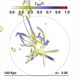
(a)

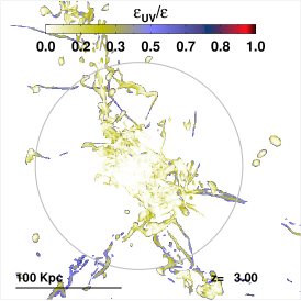
(b)

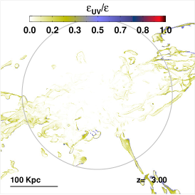
(c)

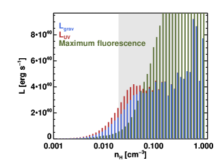
(d)

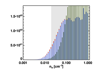
(e)

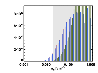
(f)

Figure 16: Top row: Fractional UV background contribution to the gas Ly$\alpha$ emissivity in the three main halos, H1, H2 and H3, from left to right. Shown are mass weighted averages along the LOS, and everything below stream densities ($0.02\mathrm{\;}{\rm{cm}}^{-3}$) is ignored. Bottom row: Density distribution of the total Ly$\alpha$ luminosity of the same halos, split into the UV (red) and the gravitational (blue) contributions. Green columns denote the Ly$\alpha$ luminosity from maximum fluorescence. The shaded area represents stream densities. Note that the histograms have different scales on the y-axes.

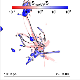
(a)

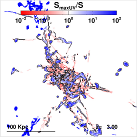
(b)

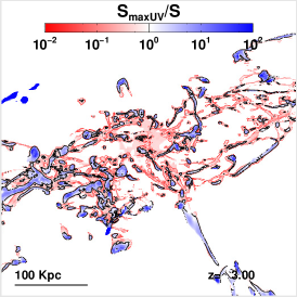
(c)

Figure 17: Ratio of the rest-frame Ly$\alpha$ surface brightness assuming maximum fluorescence (i.e. infinite UV flux, $S_{\rm maxUV}$) to our fiducial model, for halos H1, H2 and H3, from left to right. Fluorescence considerably boosts the densest clumps at the price of dimming the most diffuse streams.

5.3 Gravitational heating vs. UV fluorescence

Applying Eq. 11 we calculate the UV contribution to Ly$\alpha$ luminosity in each gas cell. We find that the relative UV contribution becomes weaker with increasing halo mass, with the ratio to the total halo Ly$\alpha$ luminosity going from $8\%$ in H1 to $2\%$ in H2 and $1\%$ in H3 (see bottom row of Fig. 7). However, the relative UV contribution is generally stronger on the edges of the halos than near their centers.

In the top row of Fig. 16 we map the fractional UV contribution to the Ly$\alpha$ emissivity in streams and CGM gas, and in the bottom row of the same figure we plot the density distribution of the total luminosity, split into the UV (red) and gravitational (blue) contributions. As the maps and histograms show, the UV contribution is negligible everywhere except for the smooth and diffuse streams with $n_{H}\la 0.05\;{\rm{cm}}^{-3}$ in the H1 halo and on the outskirts of the H2 halo. A comparison with the mock observations in Fig. 10 reveals that these diffuse streams where the UV background contribution is non-negligible are nowhere close to being observable and all the observable emission is completely dominated by the gravitational contribution. The UV background contribution to extended Ly$\alpha$ emission can thus safely be ignored, at least until the observational sensitivity increases by two orders of magnitude or so.

Inclusion of local stellar UV radiation in our simulations may boost the UV contribution, and thus both the total luminosity of the halos and the extent of observable emission. Alternatively, the presence of a luminous quasar nearby may also significantly enhance the Ly$\alpha$ luminosity through fluorescence, as demonstrated by Cantalupo et al. (2005) and Kollmeier et al. (2010).

5.4 Maximum fluorescence

Even though we lack in this work the inclusion of local sources of UV radiation, we can still evaluate the upper limit to the fluorescent Ly$\alpha$ luminosity that we can get from our simulated structures. This gives us a idea of the relative luminosity increase a local UV enhancement would provide, both in terms of the global luminosities of our halos and in terms of where the Ly$\alpha$ emissivity is boosted and where it is dimmed, compared to the gravitationally driven emission we have calculated.

To show the maximum fluorescent Ly$\alpha$ luminosities we can obtain, we re-calculate the Ly$\alpha$ emissivity of the simulated gas in the limit that $x_{\rm{H\scriptscriptstyle II}}=1$ everywhere, corresponding to an infinite flux of UV photons. Note that in this limit $\varepsilon_{coll}$ is zero everywhere and the Ly$\alpha$ emissivity is purely recombinative.

The green columns in the histograms in the bottom row of Fig. 16 show the Ly$\alpha$ luminosity of gas in different density bins in this limit. In all three halos at $n_{\rm{H}}\ga 0.1\mathrm{cm^{-3}}$, maximum fluorescence outshines the normal gas due to the increase in HII abundance, while at lower densities it is dimmer than what we predict with gravitational heating, because collisional emission goes to zero.

In Fig. 17, we show the effect of maximum fluorescence on the Ly$\alpha$ emissivity of the gas within our three simulated halos. This is displayed as the ratio of $S_{\rm maxUV}$ – the luminosity computed assuming an infinite amount of ionizing photons everywhere –, to $S$ – the luminosity used in the rest of the paper, which assumes a standard (though inhomogeneous) background value. Clearly, a strongly enhanced UV fluorescence will boost the Ly$\alpha$ emission in a significant fraction of the gas (the blue part), and may contribute significantly to LABs, as demonstrated by Cantalupo et al. (2005) and Kollmeier et al. (2010). However, from the perspective of observing accretion streams, the price to pay is the strong dimming of lower density structures (red).

This maximum fluorescence scenario is obviously optimistic, and only a tiny volume fraction of the Universe will likely come close to it, in the vicinity of rare and bright quasars in over-dense regions. Most of the IGM will more likely be in a regime comparable to our fiducial description, and its Ly$\alpha$ luminosity will be powered by collisional excitation.

6 Summary and conclusions

We have in this work addressed the questions of whether gravitational heating may be the main driver of LABs, and how close we are to making direct and unambiguous detections of cold accretion streams via their Ly$\alpha$ emission.

To this purpose we have run and analyzed cosmological RHD simulations specifically tailored to accurately predict Ly$\alpha$ emission from extended structures. These simulations are idealized in the sense that the effects of stellar feedback and Ly$\alpha$ scattering are ignored such as to isolate the efficiency of gravitational heating in generating Ly$\alpha$ photons. Our analysis is focused on redshift 3, which corresponds to most LAB observations.

Our approach improves upon previous works in the following ways: (a) Using RamsesRT, our newly developed RHD version of the Ramses code, we include on-the-fly propagation of UV photons, which allows us to consistently and accurately model the self-shielding state in accretion streams and their resulting temperatures and ionization fractions, which are all very important to accurately predict their Ly$\alpha$ emissivity. (b) We apply a novel refinement strategy that allows us to optimally resolve accretion streams to an unprecedented degree and on much larger scales than previously. This allows us to spatially resolve the competition between gravitational heating and radiative cooling in those streams. (c) We post-process our simulation outputs with very small timesteps to ensure we also resolve said competition temporally. Failing to do this leads to a dramatic underestimate of Ly$\alpha$ emissivity of gas due to the commonly utilized numerical method of operator splitting, and previous works may have been marked by this problem. (d) We simulate more massive halos than hitherto done, based on the growing consensus that LABs are hosted by the most massive halos in the Universe.

There are nontheless issues regarding uncertainties that potentially affect our results. One is the likely presence of artificial overcooling in shocks. As pointed out by Creasey et al. (2011), shocks – or the mean-free paths of particles inside them – are almost exclusively under-resolved in cosmological simulations. The artificially broadened shocks can prevent the creation of hot and diffuse gas phase and instead allow it to efficiently cool and remain at temperatures where Ly$\alpha$ emission is the most effective cooling channel. We may thus over-predict the Ly$\alpha$ emissivities of shock regions in our simulations. However, this effect should be most severe in regions where gas is shocking on to galactic disks, and should thus be mainly constrained to CGM regions, and to the densest gas under consideration, i.e. $n_{H}\sim 1\ {\rm{cm}}^{-3}{}$. Weaker shocks may also exist at the boundaries of the disrupted streams in and around our more massive halos, but it seems unlikely that numerical overcooling is a big issue here, due to the high resolution, large volumes, low densities, and the fact that the Ly$\alpha$ emissivity is not particularly concentrated at the stream boundaries.

It is an unavoidable fact that the denser the gas in our simulations, or in any simulations for that matter, the larger the uncertainty in its Ly$\alpha$ emissivity. In particular, at densities $\ga 0.1\ {\rm{cm}}^{-3}$, gas may cool down to $<<10^{4}$ K via molecular or metal-line cooling, neither of which is included in our simulations. The densest gas is also in general the most Ly$\alpha$ luminous in our simulations: What we term CGM gas ($n_{H}>0.3\ {\rm{cm}}^{-3}$) consistently accounts for $40\%$ of the total Ly$\alpha$ luminosities of our halos, so we can estimate the total Ly$\alpha$ luminosities to be uncertain by (very) roughly $50\%$, and even more if we exclude still more diffuse gas than the CGM. We have however shown that our results and conclusions regarding LAB areas are not sensitive to the density threshold applied (i.e. above which densities we ignore Ly$\alpha$ emissivity).

Our main results are the following:

• Cold accretion streams in halos more massive than $\sim 10^{12}$ M_⊙ produces extended and luminous Ly$\alpha$ nebulae which are by large compatible with LABs observed at $z\sim 3$, in terms of morphology, luminosity and extent. Gravity alone provides most of the energy, and we find that extra sources such as UV fluorescence, Ly$\alpha$ scattering or superwinds are not necessary. This clearly doesn’t rule out these other processes though, as they are likely all significant in the case of LABs, and further work is needed to study their complex interplay.

• In our simulations, LAB area and luminosity are reasonably well-behaved functions of halo mass. We use these relations to compute the cumulative luminosity and area distributions, and find that they are in reasonable agreement with observations given the relatively large uncertainties. This comparison however suggests that the combined effects of SN feedback, Ly$\alpha$ scattering and an enhanced local UV field may possibly have a negative impact on the luminosity and extent of simulated LABs, when conjoined with cold accretion.

• The model of gravitational heating as a driver of extended Ly$\alpha$ emission works according to our results, but we need to alter our notion of how it works: It is inefficient in the classic sense where gas accretion is smooth. Rather the accretion is messy and disrupted in massive halos and probably involves some mass loss to the surrounding hot diffuse medium.

• Our examination of maximum photofluorescence hints that in extreme cases local UV enhancement, e.g. near quasars, can boost the Ly$\alpha$ luminosity of LABs and to a lesser degree their extent. As demonstrated by Cantalupo et al. (2005) and Kollmeier et al. (2010), this means that large accretion flows may be more easily observed in the proximity of quasars than elsewhere.

• We find that cold accretion streams should be unambiguously observable via direct Ly$\alpha$ emission for the first time in the near future, on upcoming instruments such as MUSE and K-CWI which will allow to probe emission at surface brightnesses as low as $\sim 10^{-19}{\rm{erg\,s^{-1}\,cm^{-2}\,arcsec^{-2}}}$.

Although we have significantly improved on previous work, a large number of theoretical issues remain to be addressed. In forthcoming papers, we plan to investigate the effects of Ly$\alpha$ scattering SNe-driven winds and local UV enhancement from star formation.

Appendix A The quasi-homogeneous UV background

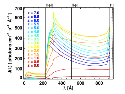
Figure 18: Evolution with redshift of the Lyman-continuum part of the UV spectrum of Faucher-Giguère et al. (2009) which we use in our simulations. The plot shows photon flux versus wavelength ($\lambda$) for selected redshifts. The vertical lines indicate how we split the spectrum into three (Hi-, Hei-, Heii-ionizing) photon packages.

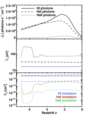
(a)

(b)

Figure 19: Left.Redshift-dependent properties of the three photon packages, integrated from the spectra in Fig. 18. Right: The redshift evolution of the photoionization rates against each species (upper plot) and per-species photo-heating rates (lower).

We use the UV background model of Faucher-Giguère et al. (2009), which is available on the web, and consists of the redshift-evolving spectrum shown in Fig. 18. As indicated by vertical lines in the plot, we discretize the spectrum into three photon packages; Hi ionizing with frequencies in the range ($\nu_{\rm{H\scriptscriptstyle I}},\nu_{\rm{He\scriptscriptstyle I}}$); Hei ionizing in the range ($\nu_{\rm{He\scriptscriptstyle I}},\nu_{\rm{He\scriptscriptstyle II}}$); and Heii ionizing in the range ($\nu_{\rm{He\scriptscriptstyle II}},\infty$). All photons belonging to a package $i$ share the common properties of flux $J_{i}$, average cross sections $\bar{\sigma}_{ij}$, where $j$ stands for the three ionizable primordial species Hi, Hei and Heii, and average energies $\bar{\epsilon}_{ij}$ per photoionization (again versus the three species). These properties are integrated from the redshift-dependent UV spectrum and updated every coarse timestep in the simulation. They are derived in the following way:

For each package $i$ that is defined for the frequency interval (${\nu_{i\scriptscriptstyle 0}},{\nu_{i\scriptscriptstyle 1}}$) and given the UV spectrum $J(\nu)\;\rm{[photons\;cm^{-2}\;s^{-1}}\;Hz^{-1}]$ (Fig. 18), we assign an average photoionization cross section against each species $j$ (Hi, Hei, Heii) as

$$\bar{\sigma}_{ij}=\frac{\int_{\nu_{i0}}^{\nu_{i1}}\sigma_{j}(\nu)J(\nu)\;d\nu}{\int_{\nu_{i0}}^{\nu_{i1}}J(\nu)\;d\nu},$$ (13)

where we use the expressions for $\sigma_{j}(\nu)$ from Hui & Gnedin (1997). Similarly, we assign to each photon package average photon energies per photoionization event against each species:

$$\bar{\epsilon}_{ij}=\frac{\int_{{\nu_{i\scriptscriptstyle 0}}}^{{\nu_{i\scriptscriptstyle 1}}}h\nu\,\sigma_{j}(\nu)J(\nu)\;d\nu}{\int_{{\nu_{i\scriptscriptstyle 0}}}^{{\nu_{i\scriptscriptstyle 1}}}\sigma_{j}(\nu)J(\nu)\;d\nu},$$ (14)

where $h$ is Planck’s constant. The flux injected isotropically into each diffuse gas cell is derived for each package as

$$J_{i}=\int_{{\nu_{i\scriptscriptstyle 0}}}^{{\nu_{i\scriptscriptstyle 1}}}J(\nu)\;d\nu.$$ (15)

When injected this way, the photons flow into adjacent cells which are above the UV density threshold and thus evolve into local photon fluxes $F^{\gamma}_{i}$ representing the quasi-homogeneous UV field. Fig. 19 shows how the package properties evolve with redshift.

Appendix B Calculating the photoionization and photo-heating rates

The hydrogen photoionization rate $\Gamma$ for the Lyman-continuum, in units of ionization events per hydrogen atom per unit time, is given by

$$\Gamma=\int_{0}^{\infty}\sigma_{\rm{H\scriptscriptstyle I}}(\nu)J(\nu)\;d\nu,$$ (16)

where $\sigma_{\rm{H\scriptscriptstyle I}}$ is the hydrogen ionization cross section and $J$ is the local photon flux, integrated over all directions. Since the UV spectrum in our RHD simulations is discretized into three photon packages, the photoionization rate is extracted from each gas cell in the simulation output as

$$\Gamma=\sum_{i=1}^{3}\bar{\sigma}_{i\rm{H\scriptscriptstyle I}}F^{\gamma}_{i},$$ (17)

where $\bar{\sigma}_{i\rm{H\scriptscriptstyle I}}$ is the average hydrogen ionization cross section for package $i$ and $F^{\gamma}_{i}$ is the local flux of package $i$ photons (see Appendix A).

 

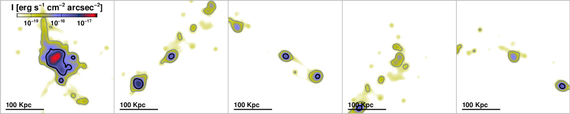
() H2

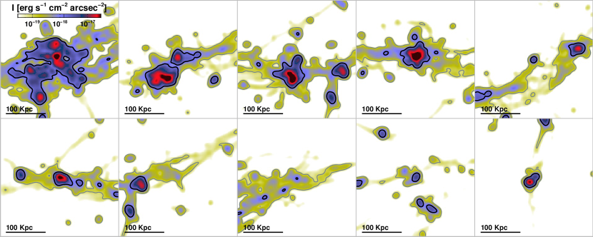
() H3

 

Figure 20: Mock observations showing $I$ for the largest objects in the H2 and H3 simulations at redshift 3, smoothed with a Gaussian PSF of FWHM=1.4 arcsec to match recent observations. The physical widths of these thumbnail squares are all identical at $300$ kpc ($\approx 40$ arcsec). The thick inner contours correspond to $I=1.4\ 10^{-18}\;{\rm{erg\,s^{-1}\,cm^{-2}\,arcsec^{-2}}}$ and the thin outer ones to $10^{-19}\;{\rm{erg\,s^{-1}\,cm^{-2}\,arcsec^{-2}}}$.

The photo-heating rate $\mathcal{H}_{\gamma}$ for the Lyman-continuum, in units of energy per time per volume, is given by

$$\mathcal{H}_{\gamma}=\sum_{j}^{\rm{{\rm{H\textsc{i}}}{},\rm{He\textsc{i}}{},\rm{He\textsc{ii}}{}}}n_{j}\int_{0}^{\infty}\sigma_{j}(\nu)F^{\gamma}(\nu)\left[h\nu-\epsilon_{j}\right]d\nu,$$ (18)

where we sum the photo-heating rates over the primordial ion species Hi, Hei and Heii. Here $n_{j}$ and is the number density of ion species $j$, $\sigma_{j}(\nu)$ is the species’ cross-section, $F^{\gamma}(\nu)$ is local photon flux, $h$ is Planck’s constant and $\epsilon_{j}$ the photoionization-threshold energies for species $j$.

With the discretization of the UV spectrum into three photon packages (see Appendix A) the integral in eq. (18) becomes a sum:

$$\mathcal{H}_{\gamma}=\sum_{j}^{\rm{{\rm{H\textsc{i}}},\rm{He\textsc{i}},\rm{He\textsc{ii}}}}n_{j}\sum_{i=1}^{3}\bar{\sigma}_{ij}F^{\gamma}_{i}\left(\bar{\epsilon}_{ij}-\epsilon_{j}\right),$$ (19)

where $F^{\gamma}_{i}$ is the local flux of photons in package $i$, and $\bar{\sigma}_{ji}$ and $\bar{\epsilon}_{ij}$ are the photon package properties defined in appendix A. We plot the redshift evolution of the per-species ionization- and heating rates in Fig. 19 (right).

Appendix C Mock LAB maps

Fig. 20 shows mock observation thumbnails of the most luminous halos in the H2 and H3 simulations, produced in the same way as the ones in Fig. 10, but applying observational parameters to match the surveys of M11 for direct comparison (these images can also be compared with thumbnails in e.g. Yang et al. 2010 and Erb et al. 2011). In practice, this means that we assume our objects are at redshift 3.1, smooth the images with a PSF with FWHM=1.4 arcsec, and put the thick inner surface brightness contours at $I=1.4\ 10^{-18}\;{\rm{erg\,s^{-1}\,cm^{-2}\,arcsec^{-2}}}$ (the thin outer ones are at $I=10^{-19}\;{\rm{erg\,s^{-1}\,cm^{-2}\,arcsec^{-2}}}$). Morphologically our mocks resemble real LABs, asymmetric with a slight tendency to be filamentary and often having short sub-filaments that poke out of the main structure. In other words, our simulated LABs look like real ones.

Appendix D Comparing the LAB luminosity function with observations

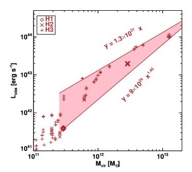
(a)

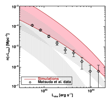
(b)

Figure 21: Left: Mock observed Ly$\alpha$ luminosities within contours of $1.4\ 10^{-18}\;{\rm{erg\,s^{-1}\,cm^{-2}\,arcsec^{-2}}}$ versus halo mass for all zoomed halos in the three simulations. Each halo is observed along three simulation box axes and thus is represented by three points in the plot. The targeted halos are marked with thick symbols. The points are enveloped by two power laws shown in the plot. Right: Predicted luminosity function of LABs (shaded region), according to the power-law envelope from the left plot. The black symbols mark a rough luminosity function derived from a sample of 202 observed LABs from the survey of M11. The horizontally and vertically line-filled regions represent predicted luminosity functions with gas densities of $n_{\rm{H}}\geq 0.3$ ${\rm{cm}}^{-3}$ and $n_{\rm{H}}\geq 0.1$ ${\rm{cm}}^{-3}$ excluded, respectively.

In Sec. 4.3.2, we derive a cumulative area function from our mock LAB observations and compare to observations. We have done the same comparison for a cumulative luminosity function, though our prediction should be less robust than the area function due to our lack of ISM modelling. Following M11, we assume $z=3.1$ and apply a PSF with FWHM=1.4. We calculate the observed Ly$\alpha$ luminosities $L_{obs}$ of all halos within the zoom regions of our simulations by integrating the surface brightness within $I=1.4\ 10^{-18}\;{\rm{erg\,s^{-1}\,cm^{-2}\,arcsec^{-2}}}$ contours. These luminosities are plotted against halo mass in Fig. 21 (left). Note the difference between $L_{obs}$ in this plot and $L$ in Fig. 8: There we plot intrinsic luminosities of halos whereas here we plot observable luminosities, assuming instrument sensitivity and cosmological extinction ($f_{\alpha}=0.66$). The plot points are enveloped by a shaded region bordered by two power laws, with indexes $1$ and $1.45$ as indicated in the plot. These power laws are convolved with a Sheth-Tormen halo mass function (Sheth & Tormen, 1999) at redshift $3.1$ in order to produce the cumulative luminosity function envelope in Fig. 21 (right).

The black diamonds in Fig. 21 (right) represent the observations from M11, derived by binning the LABs by luminosity and dividing the count by the total survey volume, with Poissonian error bars. The comparison of our results to the observations is good, somewhat surprisingly so considering the lack of modelling of the emission and absorption in the compact peaks of Ly$\alpha$ emission, which contribute substantially to the total luminosity. As with the area function, we over-predict LAB abundances, though the prediction here is slightly closer to observations than in the case of areas.

The plot also shows, with line filled regions, predicted luminosity function envelopes, where gas of densities $n_{\rm{H}}\geq 0.3$ ${\rm{cm}}^{-3}$ and $n_{\rm{H}}\geq 0.1$ ${\rm{cm}}^{-3}$ is excluded from the analysis, for the horizontal and vertical line-fillings respectively. Much as with the area function (Fig. 12), excluding CGM densities and above ($n_{\rm{H}}\geq 0.3$ ${\rm{cm}}^{-3}$) has relatively small impact on the luminosity function. However using the lower density threshold of excluding gas with $n_{\rm{H}}\geq 0.1$ ${\rm{cm}}^{-3}$ gives a very abrupt change in the function, illustrating that the simulated LAB luminosities are more sensitive to the applied density cut than their areas.

Appendix E Comparison to previous theoretical work

Our work is similar in nature to the work of FG10 and G10 (see Sec. 1), and for comparison to those we have chosen the mass of the H1 halo to be similar to the halos on which they focus their analysis.

Fig. 12 in G10 shows a plot of halo luminosities versus virial masses at redshift $3.1$, much like our Fig. 8. Their mass-luminosity power-law exponent is $\sim 0.8$, which is considerably shallower than our value of $\sim 1.25$. Their less massive halos are more luminous than ours, with our ones catching up around $10^{12}\mathrm{M_{\sun}}$. Their targeted halos of masses $\approx 4\ 10^{11}\,\mathrm{M_{\sun}}$ are typically a few times more luminous than ours, and much more extended in Ly$\alpha$ emission. Their Fig. 10 shows mock observations of two of their targeted halos. Also using $I_{-18}$ as a sensitivity limit, they have observable Ly$\alpha$ emission which is very asymmetric, clearly traces accretion streams and extends to about $100$ kpc in length.

Their prediction is probably a bit over the top, since a giant LAB in a halo of this size implies that LABs should be very common, and this contradicts the generally accepted view that they are uncommon and associated with unusually over-dense regions in the Universe (e.g. Steidel et al., 2000; Prescott et al., 2008; Yang et al., 2010). The cause of their over-prediction can probably be traced to an overestimate in gas temperatures due to their self-shielding approximation being applied in post-processing, as pointed out by FG10 (see also our Sec. 4.1).

Fig. 2 in FG10 shows a plot of halo luminosities versus halo masses at redshift $3$ for the various numerical approaches. Their estimate which is most comparable to ours (their prescription 7, that sums all gas) has a power law with exponent $\sim 1.1$, steeper than that of G10, but still a bit shallower than our exponent, and their halos are slightly Ly$\alpha$ dimmer than ours, typically around half the luminosity for a given mass, though this varies quite a lot due to scatter. The luminosity difference may be partly explained by the overdensity of our simulated regions, which tends to increase the brighness of halos of similar mass, going from the least massive to the most massive simulation. Their more conservative prescription excludes star-forming gas from their analysis, which in their simulations is gas with $n_{\rm{H}}>0.13\ {\rm{cm}}^{-3}$, likely a more realistic threshold than our $n_{\rm{H}}>1\ {\rm{cm}}^{-3}$. On this exclusion, the luminosity drops by 1-2 orders of magnitude. This is a bit more dimming than we find in our results: If the left plot of Fig. 21 is considered, where the region filled with vertical grey lines corresponds to our luminosities where gas with $n_{\rm{H}}>0.1\ {\rm{cm}}^{-3}$ is excluded from our analysis, it can be seen that the luminosity drops by $\la 1$ order of magnitude compared to our normal prescription of including all gas with $n_{\rm{H}}>1\ {\rm{cm}}^{-3}$.

They also show mock observations of a $2.5\ 10^{11}\,\mathrm{M_{\sun}}$ halo at redshift 3, that includes Ly$\alpha$ scattering. Their Fig. 7, middle left, can be compared to ours (again, their prescription 7, that sums all gas). A contour at $I_{-18}$ marks a very circular source centered on a galaxy, about $15$ kpc in diameter, which is similar to our H1 halo observation. The Ly$\alpha$ luminosity of their halo is $8\ 10^{41}$ $\mathrm{erg\,s^{-1}}$, close to the ‘observed’ luminosity of our H1 halo of $6\ 10^{41}$ $\mathrm{erg\,s^{-1}}$.

In terms of the emission coming from $\sim 10^{11}\,\mathrm{M_{\sun}}$ halos we thus seem to be in fair agreement with FG10, though the LABs produced by our simulations appear to be somewhat more luminous, even when matching their more conservative prescriptions. In terms of LAB extent it is harder to tell, since they don’t consider mock observations of halos more massive than $3\ 10^{11}\mathrm{M_{\sun}}$, and it is thus hard to tell whether or not their massive halos produce LAB-like objects.

Appendix F Table of symbols

Table 3: Table of symbols

$A$	Area
$\alpha^{\rm{B}}_{\rm{H\scriptscriptstyle I}}(T)$	Case-B recombination rate for hydrogen
$C_{{\rm{Ly}\alpha}}(T)$	Rate of collisional excitations
$\varepsilon$	Ly$\alpha$ emissivity
$\epsilon_{{\rm{Ly}\alpha}}$	Energy of a Ly$\alpha$ photon ($10.2\;\mathrm{eV}$)
${f_{\alpha}}$	Cosmological transmission factor for mock observations (we use ${f_{\alpha}}=0.66$).
$f_{c}$	Light-speed fraction
$f_{grav}$	Gravitational efficiency
$G$	Gravitational constant
$\Gamma$	Hydrogen photoionization rate
$\mathcal{H}_{\gamma}$	Photo-heating rate
$I$	Observed Ly$\alpha$ surface brightness
$I_{-18}$	Fiducial observational sensitivity limit, set to $10^{-18}$ $\mathrm{erg\,s^{-1}\,cm^{-2}\,arcsec^{-2}}$
$L$	Ly$\alpha$ luminosity
$M_{vir}$	Virial mass
$n_{\rm{H}}^{UV}$	Density threshold for UV background emitting gas
$n_{i}$	Number density of species $i$
$N_{i}$	Column density of species $i$
$r$	Radius from halo center
$R_{vir}$	Virial radius
$S$	Rest-frame Ly$\alpha$ surface brightness
$T$	Temperature
$v$	Speed
$x_{i}$	Ionization fraction of ion species $i$
$z$	Cosmological redshift

References

- Aubert et al. (2004) Aubert D., Pichon C., Colombi S., 2004, MNRAS, 352, 376
- Aubert & Teyssier (2008) Aubert D., Teyssier R., 2008, MNRAS, 387, 295
- Aubert & Teyssier (2010) Aubert D., Teyssier R., 2010, ApJ, 724, 244
- Bacon et al. (2006) Bacon R. et al., 2006, The Messenger, 124, 5
- Birnboim & Dekel (2003) Birnboim Y., Dekel A., 2003, MNRAS, 345, 349
- Birnboim et al. (2007) Birnboim Y., Dekel A., Neistein E., 2007, MNRAS, 380, 339
- Brooks et al. (2009) Brooks A. M., Governato F., Quinn T., Brook C. B., Wadsley J., 2009, ApJ, 694, 396
- Callaway et al. (1987) Callaway J., Unnikrishnan K., Oza D. H., 1987, Phys. Rev. A, 36, 2576
- Cantalupo et al. (2005) Cantalupo S., Porciani C., Lilly S. J., Miniati F., 2005, ApJ, 628, 61
- Cen (1992) Cen R., 1992, ApJS, 78, 341
- Cen (2011) Cen R., 2011, AJ, 742, L33
- Creasey et al. (2011) Creasey P., Theuns T., Bower R. G., Lacey C. G., 2011, MNRAS, 415, 3706
- Dekel & Birnboim (2006) Dekel A., Birnboim Y., 2006, MNRAS, 368, 2
- Dekel et al. (2009) Dekel A. et al., 2009, Nature, 457, 451
- Dijkstra et al. (2006) Dijkstra M., Haiman Z., Spaans M., 2006, ApJ, 649, 37
- Dijkstra & Loeb (2009) Dijkstra M., Loeb A., 2009, MNRAS, 400, 1109
- Dubois & Teyssier (2008) Dubois Y., Teyssier R., 2008, A&A, 477, 79
- Erb et al. (2011) Erb D. K., Bogosavljević M., Steidel C. C., 2011, AJ, 740, L31
- Fardal et al. (2001) Fardal M. A., Katz N., Gardner J. P., Hernquist L., Weinberg D. H., Davé R., 2001, ApJ, 562, 605