On the Complexity of the Generalized MinRank Problem

Abstract

We study the complexity of solving the generalized MinRank problem, i.e. computing the set of points where the evaluation of a polynomial matrix has rank at most $r$. A natural algebraic representation of this problem gives rise to a determinantal ideal: the ideal generated by all minors of size $r+1$ of the matrix. We give new complexity bounds for solving this problem using Gröbner bases algorithms under genericity assumptions on the input matrix. In particular, these complexity bounds allow us to identify families of generalized MinRank problems for which the arithmetic complexity of the solving process is polynomial in the number of solutions. We also provide an algorithm to compute a rational parametrization of the variety of a $0$-dimensional and radical system of bi-degree $(D,1)$. We show that its complexity can be bounded by using the complexity bounds for the generalized MinRank problem.

Keywords: MinRank, Gröbner basis, determinantal, bi-homogeneous, structured algebraic systems.

1 Introduction

We focus in this paper on the following problem:

Generalized MinRank Problem: given a field $\mathbb{K}$, a $n\times m$ matrix $\mathcal{M}$ whose entries are polynomials of degree $D$ in $\mathbb{K}[x_{1},\ldots,x_{k}]$, and $r<\min(n,m)$ an integer, compute the set of points at which the evaluation of $\mathcal{M}$ has rank at most $r$.

This problem arises in many applications and this is what motivates our study. In cryptology, the security of several multivariate cryptosystems relies on the difficulty of solving the classical MinRank problem (i.e. when the entries of the matrix are linear [28, 16, 5]). In coding theory, rank-metric codes can be decoded by computing the set of points where a polynomial matrix has rank less than a given value [33, 16]. In non-linear computational geometry, many incidence problems from enumerative geometry can be expressed by constraints on the rank of a matrix whose entries are polynomials of degree frequently larger than $1$ (see e.g. [31, 36, 35]). Also, in real geometry, optimization and quantifier elimination [34, 1, 24, 27] the critical points of a map are defined by the rank defect of its Jacobian matrix (whose entries have degrees larger than $1$ most of the time in applications). Moreover, this problem is also underlying other problems from symbolic computation (for instance solving multi-homogeneous systems, see e.g. [19]).

The ubiquity of this problem makes the development of algorithms solving it and complexity estimates of first importance. When $\mathbb{K}$ is finite, the generalized MinRank problem is known to be NP-complete [8]; thus one can consider this problem as a hard problem.

To study the Generalized MinRank problem, we consider the algebraic system of all the $(r+1)$-minors of the input matrix. Indeed, these minors simultaneously vanish on the locus of rank defect and hence give rise to a section of a determinantal ideal.

Several solving tools can be used to solve this algebraic system by taking profit of the underlying structure. For instance, the geometric resolution in [22] can use the fact that these systems can be evaluated efficiently. Also, recent works on homotopy methods [38] show that numerical algorithms can solve determinantal problems.

In this paper, we focus on Gröbner bases algorithms. A representation of the locus of rank defect is obtained by computing a lexicographical Gröbner basis by using the algorithms $F_{5}$ [14] and FGLM [15]. Indeed, experiments suggest that these algorithms take profit of the determinantal structure. The aim of this work is to give an explanation of this behavior from the viewpoint of asymptotic complexity analysis.

Related works

An important related theoretical issue is to understand the algebraic structure of the ideal $\operatorname{\mathcal{J}}_{r}\subset\mathbb{K}[U]$ (where $U$ is the set of variables $\{u_{1,1},\ldots,u_{n,m}\}$) generated by the $(r+1)$-minors of the matrix:

$$\mathcal{U}=\begin{pmatrix}u_{1,1}&\dots&u_{1,m}\\ \vdots&\ddots&\vdots\\ u_{n,1}&\dots&u_{n,m}\\ \end{pmatrix}.$$

The ideal $\operatorname{\mathcal{J}}_{r}$ has been extensively studied during last decades. In particular, explicit formulas for its degree and for its Hilbert series are known (see e.g. [21, Example 14.4.14] and [9]), as well as structural properties such as Cohen-Macaulayness and primality [25, 26].

In cryptology, [28] have proposed a multi-homogeneous algebraic modeling which can be seen as a generalization of the Lagrange multipliers and is designed as follows: a polynomial $n\times m$ matrix $\mathcal{M}\in\mathbb{K}[X]^{n\times m}$ (where $X$ denotes the set of variables $\{x_{1},\ldots,x_{k}\}$) has rank at most $r$ if and only if the dimension of its right kernel is greater than $m-r-1$. Consequently, by introducing $r(m-r)$ fresh variables $y_{1,1},\ldots,y_{r,m-r}$, we can consider the system of bi-degree $(D,1)$ in $\mathbb{K}[x_{1},\ldots,x_{k},y_{1,1},\ldots,y_{r,m-r}]$ defined by

$$\mathcal{M}\cdot\begin{pmatrix}1&0&\dots&0\\ 0&1&\dots&0\\ \vdots&\ddots&\ddots&\vdots\\ 0&0&\dots&1\\ y_{1,1}&y_{1,2}&\dots&y_{1,m-r}\\ \vdots&\vdots&\ddots&\vdots\\ y_{r,1}&y_{r,2}&\dots&y_{r,m-r}\end{pmatrix}=0.$$

If $(x_{1},\ldots,x_{k},y_{1,1},\ldots,y_{r,m-r})$ is a solution of that system, then the evaluation of the matrix $\mathcal{M}$ at the point $(x_{1},\ldots,x_{k})$ has rank at most $r$.

In [18], the case of square linear matrices is studied by performing a complexity analysis of the Gröbner bases computations. In particular, this investigation showed that the overall complexity is polynomial in the size of the matrix when the rank defect $n-r$ is constant. This theoretical analysis is supported by experimental results. The proofs were complete when the system has positive dimension, but depended on a variant of a conjecture by Fröberg in the $0$-dimensional case.

Main results

We generalize in several ways the results from [18] where only the case of square linear matrices was investigated: our contributions are the following.

• We deal with non-square matrices whose entries are polynomials of degree $D$ with generic coefficients; this is achieved by using more general tools than those considered in [18] (weighted Hilbert series). This generalization is important for applications in geometry and optimization for instance.

• When $n=(p-r)(q-r)$, the solution set of the generalized MinRank problem has dimension $0$. In that case, our proofs in this paper do not rely on Fröberg’s conjecture; this has been achieved by modifying our proof techniques and using more sophisticated and structural properties of determinantal ideals. This is important for applications in cryptology (see e.g. the sets of parameters A, B and C in the MinRank authentication scheme [10]).

Our results are complexity bounds for Gröbner bases algorithms when the input system is the set of $(r+1)$-minors of a $n\times m$ matrix $\mathcal{M}$, whose entries are polynomials of degree $D$ with generic coefficients.

By generic, we mean that there exists a non-identically null multivariate polynomial $h$ such that the complexity results hold when this polynomial does not vanish on the coefficients of the polynomials in the matrix. Therefore, from a practical viewpoint, the complexity bounds can be used for applications where the base field $\mathbb{K}$ is large enough: in that case, the probability that the coefficients of $\mathcal{M}$ do not belong to the zero set of $h$ is close to $1$.

We start by studying the homogeneous generalized MinRank problem (i.e. when the entries of $\mathcal{M}$ are homogeneous polynomials) and by proving an explicit formula for the Hilbert series of the ideal $\mathcal{I}_{r}$ generated by the $(r+1)$-minors of the matrix $\mathcal{M}$. The general framework of the proofs is the following: we consider the ideal $\operatorname{\mathcal{J}}_{r}\subset\mathbb{K}[U]$ generated by the $(r+1)$-minors of a matrix $\mathcal{U}=(u_{i,j})$ whose entries are variables. Then we consider the ideal $\widetilde{\operatorname{\mathcal{J}}_{r}}=\operatorname{\mathcal{J}}_{r}+\langle g_{1},\ldots,g_{nm}\rangle\subset\mathbb{K}[U,X]$, where the polynomials $g_{i}$ are quasi-homogeneous forms that are the sum of a linear form in $\mathbb{K}[U]$ and of a homogeneous polynomial of degree $D$ in $\mathbb{K}[X]$. If some conditions on the $g_{i}$ are verified, by performing a linear combination of the generators there exists $f_{1,1},\ldots,f_{n,m}\in\mathbb{K}[X]$ such that

$$\widetilde{\operatorname{\mathcal{J}}_{r}}=\operatorname{\mathcal{J}}_{r}+\langle u_{1,1}-f_{1,1},\ldots,u_{n,m}-f_{n,m}\rangle.$$

Then we use the fact that $\left(\operatorname{\mathcal{J}}_{r}+\langle u_{1,1}-f_{1,1},\ldots,u_{n,m}-f_{n,m}\rangle\right)\cap\mathbb{K}[X]=\mathcal{I}_{r}$ to prove that properties of generic quasi-homogeneous sections of $\operatorname{\mathcal{J}}_{r}$ transfer to $\mathcal{I}_{r}$ when the entries of the matrix $\mathcal{M}$ are generic. This allows us to use results known about the ideal $\operatorname{\mathcal{J}}_{r}$ to study the algebraic structure of $\mathcal{I}_{r}$.

We study separately three different cases:

• $k>(n-r)(m-r)$. Under genericity assumptions on the input, the solutions of the generalized MinRank problem are an algebraic variety of positive dimension. Recall that the complexity results were only proven for $D=1$ and $n=m$ in [18]. We generalize here for any $D\in\mathbb{N}$.

• $k=(n-r)(m-r)$. This is the $0-dimensional$ case, where the problem has finitely-many solutions under genericity assumptions. Recall that the results in [18] were only stated for $D=1$ and $n=m$, and they depended on a variant of Fröberg’s conjecture. In this paper, we give complete proofs for $D\in\mathbb{N}$ which do not rely on any conjecture.

• $k<(n-r)(m-r)$. In the over-determined case, we still need to assume a variant of Fröberg’s conjecture to generalize the results in [18].

In particular, we prove that, for $k\geq(n-r)(m-r)$, the Hilbert series of $\mathcal{I}_{r}$ is the power series expansion of the rational function

$$\operatorname{\sf HS}_{\mathcal{I}_{r}}(t)=\frac{\det A_{r}(t^{D})(1-t^{D})^{(n-r)(m-r)}}{t^{D\binom{r}{2}}(1-t)^{k}},$$

where $A_{r}(t)$ is the $r\times r$ matrix whose $(i,j)$-entry is $\sum_{k}\binom{m-i}{k}\binom{n-j}{k}t^{k}$. Assuming w.l.o.g. that $m\leq n$, we also prove that the degree of $\mathcal{I}_{r}$ is equal to

$$\operatorname{\sf DEG}(\mathcal{I}_{r})=D^{(n-r)(m-r)}\prod_{i=0}^{m-r-1}\frac{i!(n+i)!}{(m-1-i)!(n-r+i)!}.$$

These explicit formulas permit to derive complexity bounds on the complexity of the problem. Indeed, one way to get a representation of the solutions of the problem in the $0$-dimensional case is to compute a lexicographical Gröbner basis of the ideal generated by the polynomials. This can be achieved by using first the $F_{5}$ algorithm [14] to compute a Gröbner basis for the so-called grevlex ordering and then use the FGLM algorithm [15] to convert it into a lexicographical Gröbner basis. The complexities of these algorithms are governed by the degree of regularity and by the degree of the ideal.

Therefore the theoretical results on the structure of $\mathcal{I}_{r}$ yield bounds on the complexity of solving the generalized MinRank problem with Gröbner bases algorithms. More specifically, when $k=(n-r)(m-r)$ and under genericity assumptions on the input polynomial matrix, we prove that the arithmetic complexity for computing a lexicographical Gröbner basis of $\mathcal{I}_{r}$ is upper bounded by

$$O\left(\binom{n}{r+1}\binom{m}{r+1}\binom{\operatorname{\mathbb{D}_{reg}}+k}{k}^{\omega}+k\left(\operatorname{\sf DEG}\left(\mathcal{I}_{r}\right)\right)^{3}\right),$$

where $2\leq\omega\leq 3$ is a feasible exponent for the matrix multiplication, and

$$\operatorname{\mathbb{D}_{reg}}=Dr(m-r)+(D-1)k+1.$$

This complexity bound permits to identify families of Generalized MinRank problems for which the number of arithmetic operations during the Gröbner basis computations is polynomial in the number of solutions.

In the over-determined case (i.e. $k<(n-r)(m-r)$), we obtain similar complexity results, by assuming a variant of Fröberg’s conjecture which is supported by experiments.

Finally, we show that complexity bounds for solving systems of bi-degree $(D,1)$ can be obtained from these results on the generalized MinRank problem. We give an algorithm whose arithmetic complexity is upper bounded by

$$O\left(\binom{n_{x}+n_{y}}{n_{y}+1}\binom{D(n_{x}+n_{y})+1}{n_{x}}^{\omega}+n_{x}\left(D^{n_{x}}\binom{n_{x}+n_{y}}{n_{x}}\right)^{3}\right),$$

for solving systems of $n_{x}+n_{y}$ equations of bi-degree $(D,1)$ in $\mathbb{K}[x_{1},\ldots,x_{n_{x}},y_{1},\ldots,y_{n_{y}}]$ which are radical and $0$-dimensional.

Organization of the paper

Section 2 provides notations used throughout this paper and preliminary results. In Section 3, we show how properties of the ideal $\operatorname{\mathcal{J}}_{r}$ generated by the $(r+1)$-minors of $\mathcal{U}$ transfer to the ideal $\mathcal{I}_{r}$. Then, the case when the homogeneous Generalized MinRank Problem has non-trivial solutions (under genericity assumptions) is studied in Section 4. Section 5 is devoted to the study of the over-determined MinRank Problem (i.e. when $k<(n-r)(m-r)$). Then, the complexity analysis is performed in Section 6. Some consequences of this complexity analysis are drawn in Section 7. Experimental results are given in Section 7.4 and applications to the complexity of solving bi-homogeneous systems of bi-degree $(D,1)$ are investigated in Section 8.

2 Notations and preliminaries

Let $\mathbb{K}$ be a field and $\overline{\mathbb{K}}$ be its algebraic closure. In the sequel, $n$, $m$, $r$ and $k$ and $D$ are positive integers with $r<m\leq n$. For $d\in\mathbb{N}$, $\operatorname{Mon}(d,k)$ denotes the set of monomials of degree $d$ in the polynomial ring $\mathbb{K}[x_{1},\ldots,x_{k}]$. Its cardinality is $\#\operatorname{Mon}(d,k)=\binom{d-1+k}{d}.$

We denote by $\mathfrak{a}$ the set of parameters $\{\mathfrak{a}_{t}^{(i,j)}:1\leq i\leq n,1\leq j\leq m,t\in\operatorname{Mon}(D,k)\}$. The set of variables $\{u_{i,j}:1\leq i\leq n,1\leq j\leq m\}$ (resp. $\{x_{1},\ldots,x_{k}\}$) is denoted by $U$ (resp. $X$).

For $1\leq i\leq n,1\leq j\leq m$, we denote by $f_{i,j}\in\mathbb{K}(\mathfrak{a})[X]$ a generic form of degree $D$

$$f_{i,j}=\sum_{t\in\operatorname{Mon}(D,k)}\mathfrak{a}_{t}^{(i,j)}t.$$

Let $\mathcal{I}_{r}\subset\mathbb{K}(\mathfrak{a})[X]$ be the ideal generated by the $(r+1)$-minors of the $n\times m$ matrix

$$\mathcal{M}=\begin{pmatrix}f_{1,1}&\dots&f_{1,m}\\ \vdots&\ddots&\vdots\\ f_{n,1}&\dots&f_{n,m}\end{pmatrix},$$

and $\operatorname{\mathcal{J}}_{r}\subset\mathbb{K}(\mathfrak{a})[U,X]$ be the determinantal ideal generated by the $(r+1)$-minors of the matrix

$$\mathcal{U}=\begin{pmatrix}u_{1,1}&\dots&u_{1,m}\\ \vdots&\ddots&\vdots\\ u_{n,1}&\dots&u_{n,m}\\ \end{pmatrix}.$$

We define $\widetilde{\mathcal{I}_{r}}$ as the ideal $\operatorname{\mathcal{J}}_{r}+\langle u_{i,j}-f_{i,j}\rangle_{1\leq i\leq n,1\leq j\leq m}\subset\mathbb{K}(\mathfrak{a})[U,X]$. Notice that $\widetilde{\mathcal{I}_{r}}=\mathcal{I}_{r}+\langle u_{i,j}-f_{i,j}\rangle_{1\leq i\leq n,1\leq j\leq m}\subset\mathbb{K}(\mathfrak{a})[U,X]$. Therefore, $\mathcal{I}_{r}=\widetilde{\mathcal{I}_{r}}\cap\mathbb{K}(\mathfrak{a})[X]$.

By slight abuse of notation, if $I$ is a proper homogeneous ideal of a polynomial ring $\mathbb{K}[X]$, we call Hilbert series of $I$ and we note $\operatorname{\sf HS}_{I}\in\mathbb{Z}[[t]]$ the Hilbert series of its quotient algebra $\mathbb{K}[X]/I$ with the grading defined by $\deg(x_{i})=1$ for all $i$:

$$\operatorname{\sf HS}_{I}(t)=\sum_{d\geq 0}\dim_{\mathbb{K}}\left(\mathbb{K}[X]_{d}/I_{d}\right)t^{d},$$

where $\mathbb{K}[X]_{d}$ denotes the vector space of homogeneous polynomials of degree $d$ and $I_{d}=I\cap\mathbb{K}[X]_{d}$.

We call dimension of $I$ the Krull dimension of the quotient ring $\mathbb{K}[X]/I$.

Quasi-homogeneous polynomials.

We need to balance the degrees of the entries of the matrix $\mathcal{U}$ with the degrees of the entries of $\mathcal{M}$. This can be achieved by putting a weight on the variables $u_{i,j}$, giving rise to quasi-homogeneous polynomials. A polynomial $f\in\mathbb{K}[U,X]$ is called quasi-homogeneous (of type $(D,1)$) if the following condition holds (see e.g. [23, Definition 2.11, page 120]):

$$f(\lambda^{D}u_{1,1},\ldots,\lambda^{D}u_{n,m},\lambda x_{1},\ldots,\lambda x_{k})=\lambda^{d}f(u_{1,1},\ldots,u_{n,m},x_{1},\ldots,x_{k}).$$

The integer $d$ is called the weight degree of $f$ and denoted by $\operatorname{wdeg}(f)$.

An ideal $I\subset\mathbb{K}[U,X]$ is called quasi-homogeneous (of type $(D,1)$) if there exists a set of quasi-homogeneous generators. In this case, we denote by $\mathbb{K}[U,X]_{d}$ the $\mathbb{K}$-vector space of quasi-homogeneous polynomials of weight degree $d$, and $I_{d}$ denote the set $\mathbb{K}[U,X]_{d}\cap I$.

Proposition 1.

Let $I\subset\mathbb{K}[U,X]$ be an ideal. Then the following statements are equivalent:

1. there exists a set of quasi-homogeneous generators of $I$;

2. the sets $I_{d}$ are subspaces of $\mathbb{K}[U,X]_{d}$, and $I=\bigoplus_{d\in\mathbb{N}}I_{d}$.

Proof.

See e.g. [32, Chapter 8]. ∎

If $I$ is a quasi-homogeneous ideal, then its weighted Hilbert series $\operatorname{\sf wHS}_{I}(t)\in\mathbb{Z}[[t]]$ is defined as follows:

$$\operatorname{\sf wHS}_{I}(t)=\sum_{d\in\mathbb{N}}\dim(\mathbb{K}[U,X]_{d}/I_{d})t^{d}.$$

3 Transferring properties from $\operatorname{\mathcal{J}}_{r}$ to $\mathcal{I}_{r}$

In this section, we prove that generic structural properties (such as the dimension, the structure of the leading monomial ideal,…) of the ideal $\widetilde{\mathcal{I}_{r}}$ are the same as properties of the ideal $\operatorname{\mathcal{J}}_{r}$ where several generic forms have been added. Hence several classical properties of the determinantal ideal $\operatorname{\mathcal{J}}_{r}$ transfer to the ideal $\widetilde{\mathcal{I}_{r}}$. For instance, this technique permits to obtain explicit forms of the Hilbert series of the ideal $\widetilde{\mathcal{I}_{r}}$.

In the following, we denote by $\mathfrak{b}$ and $\mathfrak{c}$ the following sets of parameters:

$$\begin{array}[]{rcl}\mathfrak{b}&=&\{\mathfrak{b}^{(\ell)}_{t}\mid t\in\operatorname{Mon}(D,k),1\leq\ell\leq nm\};\\ \mathfrak{c}&=&\{\mathfrak{c}^{(\ell)}_{i,j}\mid 1\leq i\leq n,1\leq j\leq m,1\leq\ell\leq nm\}.\end{array}$$

Also, $g_{1},\ldots,g_{nm}\in\mathbb{K}(\mathfrak{b},\mathfrak{c})[U,X]$ are generic quasi-homogeneous forms of type $(D,1)$ and of weight degree $D$:

$$g_{\ell}=\sum_{t\in\operatorname{Mon}(D,k)}\mathfrak{b}_{t}^{(\ell)}t+\sum_{\begin{subarray}{c}1\leq i\leq n\\ 1\leq j\leq m\end{subarray}}\mathfrak{c}_{i,j}^{(\ell)}u_{i,j}.$$

We let $\widetilde{\operatorname{\mathcal{J}}_{r}}$ denote the ideal $\operatorname{\mathcal{J}}_{r}+\langle g_{1},\ldots,g_{nm}\rangle\subset\mathbb{K}(\mathfrak{b},\mathfrak{c})[U,X]$. Here and subsequently, for $\mathbf{a}=(a_{i,j})\in\overline{\mathbb{K}}^{nm\binom{D-1+k}{D}}$, we denote by $\varphi_{\mathbf{a}}$ the following evaluation morphism:

$$\begin{array}[]{cccc}\varphi_{\bf a}:&\mathbb{K}[\mathfrak{a}]&\longrightarrow&\overline{\mathbb{K}}\\ &f(\mathfrak{a}_{1,1},\ldots,\mathfrak{a}_{n,m})&\longmapsto&f(a_{1,1},\ldots,a_{n,m})\end{array}$$

Also, for $(\mathbf{b},\mathbf{c})\in\overline{\mathbb{K}}^{nm\left(\binom{D-1+k}{D}+nm\right)}$, we denote by $\psi_{\mathbf{b},\mathbf{c}}$ the evaluation morphism:

$$\begin{array}[]{cccc}\psi_{\mathbf{b},\mathbf{c}}:&\mathbb{K}[\mathfrak{b},\mathfrak{c}]&\longrightarrow&\overline{\mathbb{K}}\\ &f(\mathfrak{b},\mathfrak{c})&\longmapsto&f(\mathbf{b},\mathbf{c})\end{array}$$

By abuse of notation, we let $\varphi_{\mathbf{a}}(\widetilde{\mathcal{I}_{r}})$ (resp. $\psi_{\mathbf{b},\mathbf{c}}(\widetilde{\operatorname{\mathcal{J}}_{r}})$) denote the ideal $\operatorname{\mathcal{J}}_{r}+\langle u_{i,j}-\varphi_{\bf a}(f_{i,j})\rangle\subset\overline{\mathbb{K}}[U,X]$ (resp. $\operatorname{\mathcal{J}}_{r}+\left\langle\psi_{\mathbf{b},\mathbf{c}}(g_{1}),\ldots,\psi_{\mathbf{b},\mathbf{c}}(g_{nm})\right\rangle\subset\overline{\mathbb{K}}[U,X]$).

We call property a map from the set of ideals of $\overline{\mathbb{K}}[U,X]$ to $\{{\tt true},{\tt false}\}$:

$$\begin{array}[]{rrcl}\mathcal{P}:&\mathsf{Ideals}(\overline{\mathbb{K}}[U,X])&\rightarrow&\{{\tt true},{\tt false}\}\end{array}.$$

Definition 1.

Let $\mathcal{P}$ be a property. We say that $\mathcal{P}$ is

• $\widetilde{\mathcal{I}_{r}}$-generic if there exists a non-empty Zariski open subset $O\subset\overline{\mathbb{K}}^{nm\binom{D-1+k}{D}}$ such that

  $$\mathbf{a}\in O\Rightarrow\mathcal{P}\left(\varphi_{\mathbf{a}}\left(\widetilde{\mathcal{I}_{r}}\right)\right)={\tt true};$$

• $\widetilde{\operatorname{\mathcal{J}}_{r}}$-generic if there exists a non-empty Zariski open subset $O\subset\overline{\mathbb{K}}^{nm\left(\binom{D-1+k}{D}+nm\right)}$ such that

  $$(\mathbf{b},\mathbf{c})\in O\Rightarrow\mathcal{P}\left(\psi_{\mathbf{b},\mathbf{c}}\left(\widetilde{\operatorname{\mathcal{J}}_{r}}\right)\right)={\tt true}.$$

The following lemma is the main result of this section:

Lemma 1.

A property $\mathcal{P}$ is $\widetilde{\mathcal{I}_{r}}$-generic if and only if it is $\widetilde{\operatorname{\mathcal{J}}_{r}}$-generic.

Proof.

To obtain a representation of $\varphi_{\bf a}\left(\widetilde{\operatorname{\mathcal{J}}_{r}}\right)$ for a generic $\mathbf{a}$ as a specialization of $\widetilde{\mathcal{I}_{r}}$ (and conversely), it is sufficient to perform a linear combination of the generators. The point of this proof is to show that genericity is preserved during this linear transform.

In the sequel we denote by $\mathfrak{A},\mathfrak{B}$ and $\mathfrak{C}$ the following matrices (of respective sizes $nm\times\binom{D-1+k}{D}$, $nm\times\binom{D-1+k}{D}$ and $nm\times nm$):

$$\begin{array}[]{rcl}\mathfrak{A}&=&\begin{pmatrix}\mathfrak{a}^{(1)}_{x_{1}^{D}}&\mathfrak{a}^{(1)}_{x_{1}^{D-1}x_{2}}&\dots&\mathfrak{a}^{(1)}_{x_{k}^{D}}\\ \vdots&\vdots&\vdots&\vdots\\ \mathfrak{a}^{(nm)}_{x_{1}^{D}}&\mathfrak{a}^{(nm)}_{x_{1}^{D-1}x_{2}}&\dots&\mathfrak{a}^{(nm)}_{x_{k}^{D}}\end{pmatrix}\\ \mathfrak{B}&=&\begin{pmatrix}\mathfrak{b}^{(1)}_{x_{1}^{D}}&\mathfrak{b}^{(1)}_{x_{1}^{D-1}x_{2}}&\dots&\mathfrak{b}^{(1)}_{x_{k}^{D}}\\ \vdots&\vdots&\vdots&\vdots\\ \mathfrak{b}^{(nm)}_{x_{1}^{D}}&\mathfrak{b}^{(nm)}_{x_{1}^{D-1}x_{2}}&\dots&\mathfrak{b}^{(nm)}_{x_{k}^{D}}\end{pmatrix}\\ \mathfrak{C}&=&\begin{pmatrix}\mathfrak{c}^{(1)}_{1,1}&\dots&\mathfrak{c}^{(1)}_{n,m}\\ \vdots&\vdots&\vdots\\ \mathfrak{c}^{(nm)}_{1,1}&\dots&\mathfrak{c}^{(nm)}_{n,m}\end{pmatrix}.\end{array}$$

Therefore, we have

$$\begin{array}[]{rcl}\begin{pmatrix}u_{1,1}-f_{1,1}\\ \vdots\\ u_{n,m}-f_{n,m}\end{pmatrix}&=&\mathsf{Id}_{nm}\cdot\begin{pmatrix}u_{1,1}\\ \vdots\\ u_{n,m}\end{pmatrix}-\mathfrak{A}\cdot\begin{pmatrix}x_{1}^{D}\\ x_{1}^{D-1}x_{2}\\ \vdots\\ x_{k}^{D}\end{pmatrix}\\ \begin{pmatrix}g_{1}\\ \vdots\\ g_{nm}\end{pmatrix}&=&\mathfrak{C}\cdot\begin{pmatrix}u_{1,1}\\ \vdots\\ u_{n,m}\end{pmatrix}+\mathfrak{B}\cdot\begin{pmatrix}x_{1}^{D}\\ x_{1}^{D-1}x_{2}\\ \vdots\\ x_{k}^{D}\end{pmatrix}\end{array}$$

In this proof, for $\mathbf{a}\in\mathbb{K}^{nm\binom{D-1+k}{D}}$ (resp. $\mathbf{b}\in\mathbb{K}^{nm\binom{D-1+k}{D}},\mathbf{c}\in\mathbb{K}^{n^{2}m^{2}}$), the notation $\mathbf{A}$ (resp. $\mathbf{B},\mathbf{C}$) stands for the evaluation of the matrix $\mathfrak{A}$ (resp. $\mathfrak{B},\mathfrak{C}$) at $\mathbf{a}$ (resp. $\mathbf{b},\mathbf{c}$). Also, we implicitly identify $\mathbf{A}$ with $\mathbf{a}$ (resp. $\mathbf{B}$ with $b$, $\mathbf{C}$ with $\mathbf{c}$, $\mathfrak{A}$ with $\mathfrak{a}$, $\mathfrak{B}$ with $\mathfrak{b}$, $\mathfrak{C}$ with $\mathfrak{c}$).

• Let $\mathcal{P}$ be a $\widetilde{\mathcal{I}_{r}}$-generic property. Thus there exists a non-zero polynomial $h_{1}(\mathfrak{A})\in\overline{\mathbb{K}}[\mathfrak{a}]$ such that if $h_{1}(\mathbf{A})\neq 0$ then $\mathcal{P}\left(\varphi_{\mathbf{a}}(\widetilde{\mathcal{I}_{r}})\right)={\tt true}$.

  Let $\mathsf{adj}(\mathfrak{C})$ denote the adjugate of $\mathfrak{C}$ (i.e. $\mathsf{adj}(\mathfrak{C})=\det(\mathfrak{C})\cdot\mathfrak{C}^{-1}$ in $\mathbb{K}(\mathfrak{c})$). Consider the polynomial $\widetilde{h_{1}}$ defined by $\widetilde{h_{1}}(\mathfrak{B},\mathfrak{C})=h_{1}(-\mathsf{adj}(\mathfrak{C})\cdot\mathfrak{B})\in\overline{\mathbb{K}}[\mathfrak{b},\mathfrak{c}]$. The polynomial inequality $\det(\mathfrak{C})\widetilde{h_{1}}(\mathfrak{B},\mathfrak{C})\neq 0$ defines a non-empty Zariski open subset $O\subset\overline{\mathbb{K}}^{nm\left(\binom{D-1+k}{D}+nm\right)}.$ Let $(\mathbf{B},\mathbf{C})\in O$ be an element in this set, then $\mathbf{C}$ is invertible since $\det(\mathbf{C})\neq 0$. Let $\widetilde{\mathbf{A}}$ be the matrix $\widetilde{\mathbf{A}}=-\mathsf{adj}(\mathbf{C})\cdot\mathbf{B}$. Therefore the generators of the ideal $\varphi_{\widetilde{\mathbf{a}}}\left(\widetilde{\mathcal{I}_{r}}\right)$ are an invertible linear combination of the generators of $\psi_{\mathbf{b},\mathbf{c}}\left(\widetilde{\operatorname{\mathcal{J}}_{r}}\right)$. Consequently, $\varphi_{\widetilde{\mathbf{a}}}\left(\widetilde{\mathcal{I}_{r}}\right)=\psi_{\mathbf{b},\mathbf{c}}\left(\widetilde{\operatorname{\mathcal{J}}_{r}}\right)$. Moreover, $h_{1}(\widetilde{\bf A})=\widetilde{h_{1}}(\mathbf{B},\mathbf{C})\neq 0$ implies that the polynomial $\widetilde{h_{1}}$ is not identically $0$. Therefore,

  $$\forall(\mathbf{b},\mathbf{c})\in O,\mathcal{P}\left(\psi_{\mathbf{b},\mathbf{c}}\left(\widetilde{\operatorname{\mathcal{J}}_{r}}\right)\right)=\mathcal{P}\left(\varphi_{\widetilde{\mathbf{a}}}\left(\widetilde{\mathcal{I}_{r}}\right)\right)={\tt true},$$

  and hence $\mathcal{P}$ is a $\widetilde{\operatorname{\mathcal{J}}_{r}}$-generic property.

• Conversely, consider a $\widetilde{\operatorname{\mathcal{J}}_{r}}$-generic property $\mathcal{P}$. Thus, there exists a non-zero polynomial $h_{2}(\mathfrak{B},\mathfrak{C})\in\overline{\mathbb{K}}[\mathfrak{b},\mathfrak{c}]$ such that if $h_{2}(\mathbf{b},\mathbf{c})\neq 0$ then $\mathcal{P}\left(\psi_{\mathbf{b},\mathbf{c}}(\widetilde{\operatorname{\mathcal{J}}_{r}})\right)={\tt true}$. Since $\mathcal{P}$ is $\widetilde{\operatorname{\mathcal{J}}_{r}}$-generic, there exists $(\mathbf{b},\mathbf{c})$ such that $h_{2}(\mathbf{b},\mathbf{c})\det(\mathbf{c})\neq 0$. Let $\widetilde{h_{2}}$ be the polynomial $\widetilde{h_{2}}(\mathfrak{b})=h_{2}(-\mathbf{C}\cdot\mathfrak{B},\mathbf{C})$.

  Since $\det(\mathbf{C})\neq 0$, the matrix $\mathbf{C}$ is invertible and $\widetilde{h_{2}}(-\mathbf{C}^{-1}\cdot\mathbf{B})=h_{2}(\mathbf{B},\mathbf{C})\neq 0$ and hence the polynomial $\widetilde{h_{2}}$ is not identically $0$. Moreover, if $\mathbf{a}\in\mathbb{K}^{nm\binom{D-1+k}{D}}$ is such that $\widetilde{h_{2}}(\mathbf{A})\neq 0$, then $h_{2}(-\mathbf{C}\cdot\mathbf{A},\mathbf{C})\neq 0$ and thus $\mathcal{P}\left(\psi_{-\mathbf{C}\cdot\mathbf{A},\mathbf{C}}(\widetilde{\operatorname{\mathcal{J}}_{r}})\right)={\tt true}$. Finally, $\psi_{-\mathbf{C}\cdot\mathbf{A},\mathbf{C}}(\widetilde{\operatorname{\mathcal{J}}_{r}})=\varphi_{\mathbf{A}}(\widetilde{\mathcal{I}_{r}})$ since the generators of $\psi_{-\mathbf{C}\cdot\mathbf{A},\mathbf{C}}(\widetilde{\operatorname{\mathcal{J}}_{r}})$ are an invertible linear combination of that of $\varphi_{\mathbf{a}}(\widetilde{\mathcal{I}_{r}})$ (the linear transformation being given by the invertible matrix $\mathbf{C}$) and hence they generate the same ideal. Therefore, the property $\mathcal{P}$ is $\widetilde{\mathcal{I}_{r}}$-generic.

∎

In the sequel, $\prec$ is an admissible monomial ordering (see e.g [11, Chapter 2, §2, Definition 1]) on $\mathbb{K}[U,X]$, and for any polynomial $f\in\mathbb{K}[U,X]$, $\operatorname{\sf LM}(f)$ denotes its leading monomial with respect to $\prec$. If $I$ is an ideal of $\mathbb{K}[U,X]$, $\mathbb{K}(\mathfrak{a})[U,X]$, or $\mathbb{K}(\mathfrak{b},\mathfrak{c})[U,X]$, we let $\operatorname{\sf LM}(I)$ denote the ideal generated by the leading monomials of the polynomials.

By slight abuse of notation, if $I_{1}$ and $I_{2}$ are ideals of $\mathbb{K}[U,X]$, $\mathbb{K}(\mathfrak{a})[U,X]$, or $\mathbb{K}(\mathfrak{b},\mathfrak{c})[U,X]$ ($I_{1}$ and $I_{2}$ are not necessarily ideals of the same ring), we write $\operatorname{\sf LM}(I_{1})=\operatorname{\sf LM}(I_{2})$ if the sets $\{\operatorname{\sf LM}(f)\mid f\in I_{1}\}$ and $\{\operatorname{\sf LM}(f)\mid f\in I_{2}\}$ are equal.

Lemma 2.

Let $\mathcal{P}_{\widetilde{\mathcal{I}_{r}}}$ and $\mathcal{P}_{\widetilde{\operatorname{\mathcal{J}}_{r}}}$ be the properties defined by

$$\begin{array}[]{c}\mathcal{P}_{\widetilde{\mathcal{I}_{r}}}(I)=\begin{cases}{\tt true}\text{ if }\operatorname{\sf LM}(I)=\operatorname{\sf LM}\left(\widetilde{\mathcal{I}_{r}}\right);\\ {\tt false}\text{ otherwise.}\end{cases}\\ \mathcal{P}_{\widetilde{\operatorname{\mathcal{J}}_{r}}}(I)=\begin{cases}{\tt true}\text{ if }\operatorname{\sf LM}(I)=\operatorname{\sf LM}\left(\widetilde{\operatorname{\mathcal{J}}_{r}}\right);\\ {\tt false}\text{ otherwise.}\end{cases}\end{array}$$

Then $\mathcal{P}_{\widetilde{\mathcal{I}_{r}}}$ (resp. $\mathcal{P}_{\widetilde{\operatorname{\mathcal{J}}_{r}}}$) is a $\widetilde{\mathcal{I}_{r}}$-generic (resp. $\widetilde{\operatorname{\mathcal{J}}_{r}}$-generic) property.

Proof.

We prove here that $\mathcal{P}_{\widetilde{\mathcal{I}_{r}}}$ is $\widetilde{\mathcal{I}_{r}}$-generic (the proof for $\mathcal{P}_{\widetilde{\operatorname{\mathcal{J}}_{r}}}$ is similar).

The outline of this proof is the following: during the computation of a Gröbner basis $G$ of $\widetilde{\mathcal{I}_{r}}$ in $\mathbb{K}(\mathfrak{a})[U,X]$ (for instance with Buchberger’s algorithm), a finite number of polynomials are constructed. Let $\varphi_{\mathbf{a}}$ be a specialization. If the images by $\varphi_{\mathbf{a}}$ of the leading coefficients of all non-zero polynomials arising during the computation do not vanish, then $\varphi_{\mathbf{a}}(G)\subset\varphi_{\mathbf{a}}(\widetilde{\mathcal{I}_{r}})$ is a Gröbner basis of the ideal it generates. It remains to prove that $\varphi_{\mathbf{a}}(G)$ is a Gröbner basis of $\varphi_{\mathbf{a}}(\widetilde{\mathcal{I}_{r}})$. This is achieved by showing that generically, the normal form (with respect to $\varphi_{\mathbf{a}}(G)$) of the generators of $\varphi_{\mathbf{a}}(\widetilde{\mathcal{I}_{r}})$ is equal to zero.

For polynomials $f_{1},f_{2}$, we let $\operatorname{\sf LC}(f_{1})$ (resp. $\operatorname{\sf LC}(f_{2})$) denote the leading coefficient of $f_{1}$ (resp. $f_{2}$) and $\operatorname{\sf Spol}(f_{1},f_{2})=\frac{\mathsf{LCM}(\operatorname{\sf LM}(f_{1}),\operatorname{\sf LM}(f_{2}))}{\operatorname{\sf LC}(f_{1})\operatorname{\sf LM}(f_{1})}f_{1}-\frac{\mathsf{LCM}(\operatorname{\sf LM}(f_{1}),\operatorname{\sf LM}(f_{2}))}{\operatorname{\sf LC}(f_{2})\operatorname{\sf LM}(f_{2})}f_{2}$ denote the S-polynomial of $f_{1}$ and $f_{2}$.

We need to prove that there exists a non-empty Zariski open subset $O_{1}\subset\overline{\mathbb{K}}^{nm\binom{D-1+k}{D}}$ such that

$$\mathbf{a}\in O_{1}\Rightarrow\operatorname{\sf LM}(\varphi_{\bf a}(\widetilde{\mathcal{I}_{r}}))=\operatorname{\sf LM}(\widetilde{\mathcal{I}_{r}}).$$

To do so, consider a Gröbner basis $G\subset\mathbb{K}(\mathfrak{a})[U,X]$ of $\widetilde{\mathcal{I}_{r}}$ such that each polynomial $g$ can be written as a combination $g=\sum h_{\ell}f_{\ell}$, where the $f_{\ell}$’s range over the set of minors of size $r+1$ of $\mathcal{U}$ and the polynomials $u_{i,j}-f_{i,j}$, and $h_{\ell}\in\mathbb{K}[\mathfrak{a}][U,X]$. Buchberger’s criterion states that S-polynomials of polynomials in a Gröbner basis reduce to zero [11, Chapter 2, §6, Theorem 6]. Thus each S-polynomial of $g_{i},g_{j}\in G$ can be rewritten as an algebraic combination

$$\operatorname{\sf Spol}(g_{i},g_{j})=\sum_{\ell}h_{\ell}^{\prime}g_{\ell},$$

where the polynomials $h_{\ell}^{\prime}$ belongs to $\mathbb{K}(\mathfrak{a})[U,X]$ and such that $\{g_{1},\ldots,g_{t_{i,j}}\}\subset G$ and for each $1\leq s\leq t_{i,j}$, $\operatorname{\sf LM}(g_{s})$ divides $\operatorname{\sf LM}(\operatorname{\sf Spol}(g,g^{\prime})-\sum_{\ell=1}^{s-1}h_{\ell}^{\prime}g_{\ell})$. Next, consider:

• the product $Q_{1}(\mathfrak{a})=\prod_{g\in G}\operatorname{\sf LC}(g)$ of the leading coefficients of the polynomials in the Gröbner basis;

• for all $(g_{i},g_{j})\in G^{2}$ such that $\operatorname{\sf Spol}(g_{i},g_{j})\neq 0$, the product $Q_{2}(\mathfrak{a})$ of the numerators and denominators of the leading coefficients arising during the reduction of $\operatorname{\sf Spol}(g_{i},g_{j})$.

These coefficients belongs to $\mathbb{K}[\mathfrak{a}]$. Denote by $Q(\mathfrak{a})=Q_{1}(\mathfrak{a})Q_{2}(\mathfrak{a})\in\mathbb{K}[\mathfrak{a}]$ their product. The inequality $Q(\mathfrak{a})\neq 0$ defines a non-empty Zariski open subset $O_{1}\subset\overline{\mathbb{K}}^{nm\binom{D-1+k}{D}}$. If $\mathbf{a}\in O_{1}$, then

$$\varphi_{\bf a}(\operatorname{\sf Spol}(g,g^{\prime}))=\sum_{\ell=1}^{t}\varphi_{\bf a}(h_{\ell}^{\prime})\varphi_{\bf a}(g_{\ell}),$$

and for each $1\leq i\leq t$, $\operatorname{\sf LM}(\varphi_{\bf a}(g_{i}))$ divides $\operatorname{\sf LM}(\varphi_{\bf a}(\operatorname{\sf Spol}(g,g^{\prime}))-\sum_{\ell=1}^{i-1}\varphi_{\bf a}(h_{\ell}^{\prime})\varphi_{\bf a}(g_{\ell}))$. Thus $\varphi_{\bf a}(G)$ is a Gröbner basis of the ideal it spans. Moreover, $\langle\varphi_{\bf a}(G)\rangle\subset\varphi_{\bf a}(\widetilde{\mathcal{I}_{r}})$.

We prove now that there exists a non-empty Zariski open set where the other inclusion $\varphi_{\bf a}(\widetilde{\mathcal{I}_{r}})\subset\langle\varphi_{\bf a}(G)\rangle$ holds. Let $\operatorname{\sf NF}_{G}(\cdot)$ be the normal form associated to this Gröbner basis (as defined as the remainder of the division by $G$ in [11, Chapter 2, §6, Proposition 1]). For each generator $f$ of $\widetilde{\mathcal{I}_{r}}$ (i.e. either a maximal minor of the matrix $\mathcal{U}$, or a polynomial $u_{i,j}-f_{i,j}$), we have that $\operatorname{\sf NF}_{G}(f)=0$. During the computation of $\operatorname{\sf NF}_{G}(f)$ by using the division Algorithm in [11, Chapter 2, §3], a finite set of polynomials (in $\mathbb{K}(\mathfrak{a})[U,X]$) is constructed. Let $Q_{3}\in\mathbb{K}[\mathfrak{a}]$ denote the product of the numerators and denominators of all their nonzero coefficients. Consequently, if $Q_{3}^{(f)}(\mathbf{a})\neq 0$, then $\operatorname{\sf NF}_{\varphi_{\bf a}(G)}(\varphi_{\bf a}(f))=0$ and hence $\varphi_{\bf a}(f)\in\langle\varphi_{\bf a}(G)\rangle$. Repeating this operation for all the generators of $\widetilde{\mathcal{I}_{r}}$ yields a finite set of non-identically null polynomials $Q_{3}^{(f)}\in\mathbb{K}[\mathfrak{a}]$. Let $Q_{4}\in\mathbb{K}[\mathfrak{a}]$ denote their product. Therefore, if $Q_{4}(\mathbf{a})\neq 0$, then $\varphi_{\bf a}(\widetilde{\mathcal{I}_{r}})\subset\langle\varphi_{\bf a}(G)\rangle$.

Finally, consider the non-empty Zariski open subset $O\subset\mathbb{K}^{nm\binom{D+k-1}{D}}$ defined by the inequality $Q_{1}\cdot Q_{2}\cdot Q_{4}\neq 0$. For all $\mathbf{a}\in O$, we have $\varphi_{\bf a}(\widetilde{\mathcal{I}_{r}})=\langle\varphi_{\bf a}(G)\rangle$.

∎

Corollary 1.

The leading monomials of $\widetilde{\mathcal{I}_{r}}$ are the same as that of $\widetilde{\operatorname{\mathcal{J}}_{r}}$:

$$\operatorname{\sf LM}\left(\widetilde{\mathcal{I}_{r}}\right)=\operatorname{\sf LM}\left(\widetilde{\operatorname{\mathcal{J}}_{r}}\right).$$

Proof.

By Lemmas 1 and 2, the property $\mathcal{P}_{\widetilde{\mathcal{I}_{r}}}$ (resp. $\mathcal{P}_{\widetilde{\operatorname{\mathcal{J}}_{r}}}$) is $\widetilde{\mathcal{I}_{r}}$-generic and $\widetilde{\operatorname{\mathcal{J}}_{r}}$-generic. Since $\mathcal{P}_{\widetilde{\operatorname{\mathcal{J}}_{r}}}$ (resp. $\mathcal{P}_{\widetilde{\mathcal{I}_{r}}}$) is $\widetilde{\operatorname{\mathcal{J}}_{r}}$-generic, there exists a non-empty Zariski open subset $O_{1}\subset\overline{\mathbb{K}}^{nm\left(\binom{D-1+k}{D}+nm\right)}$ (resp. $O_{2}\subset\overline{\mathbb{K}}^{nm\left(\binom{D-1+k}{D}+nm\right)}$) such that, for $(\mathbf{b},\mathbf{c})\in O_{1}$ (resp. $O_{2}$), $\operatorname{\sf LM}\left(\psi_{(\mathbf{b},\mathbf{c})}(\widetilde{\operatorname{\mathcal{J}}_{r}})\right)=\operatorname{\sf LM}\left(\widetilde{\operatorname{\mathcal{J}}_{r}}\right)$ (resp. $\operatorname{\sf LM}\left(\psi_{(\mathbf{b},\mathbf{c})}(\widetilde{\operatorname{\mathcal{J}}_{r}})\right)=\operatorname{\sf LM}\left(\widetilde{\mathcal{I}_{r}}\right)$).

Notice that $O_{1}\cap O_{2}$ is not empty, since for the Zariski topology, the intersection of finitely-many non-empty open subsets is non-empty. Let $(\mathbf{b},\mathbf{c})$ be an element of $O_{1}\cap O_{2}$. Then

$$\operatorname{\sf LM}\left(\widetilde{\mathcal{I}_{r}}\right)=\operatorname{\sf LM}\left(\psi_{(\mathbf{b},\mathbf{c})}(\widetilde{\operatorname{\mathcal{J}}_{r}})\right)=\operatorname{\sf LM}\left(\widetilde{\operatorname{\mathcal{J}}_{r}}\right).$$

∎

Corollary 2.

The weighted Hilbert series of $\widetilde{\mathcal{I}_{r}}$ is the same as that of $\widetilde{\operatorname{\mathcal{J}}_{r}}$.

Proof.

It is well-known that, for any positively graded ideal $I$ and for any monomial ordering, $\operatorname{\sf wHS}_{I}(t)=\operatorname{\sf wHS}_{\operatorname{\sf LM}(I)}(t)$ (see e.g. the proof of [11, Chapter 9, §3, Proposition 9] which is also valid for quasi-homogeneous ideals). By Corollary 1, $\operatorname{\sf LM}\left(\widetilde{\mathcal{I}_{r}}\right)=\operatorname{\sf LM}\left(\widetilde{\operatorname{\mathcal{J}}_{r}}\right)$, which implies that

$$\operatorname{\sf wHS}_{\operatorname{\sf LM}\left(\widetilde{\mathcal{I}_{r}}\right)}(t)=\operatorname{\sf wHS}_{\operatorname{\sf LM}\left(\widetilde{\operatorname{\mathcal{J}}_{r}}\right)}(t),$$

and hence $\operatorname{\sf wHS}_{\widetilde{\mathcal{I}_{r}}}(t)=\operatorname{\sf wHS}_{\widetilde{\operatorname{\mathcal{J}}_{r}}}(t)$. ∎

4 The case $k\geq(n-r)(m-r)$

As we will see in the sequel, the Krull dimension of the ring $\mathbb{K}(\mathfrak{a})[X]/\mathcal{I}_{r}$ is equal to $\max(k-(n-r)(m-r),0)$. This section is devoted to the study of the case $k\geq(n-r)(m-r)$.

We show here that the algebraic structure of the ideal $\mathcal{I}_{r}$ is closely related to that of a generic section of a determinantal variety.

We recall that the polynomials $g_{\ell}$ are defined by

$$g_{\ell}=\sum_{t\in\operatorname{Mon}(D,k)}\mathfrak{b}_{t}^{(\ell)}t+\sum_{\begin{subarray}{c}1\leq i\leq n\\ 1\leq j\leq m\end{subarray}}\mathfrak{c}_{i,j}^{(\ell)}u_{i,j}.$$

Lemma 3.

Let $1\leq\ell\leq nm$ be an integer. If $g_{\ell}$ divides zero in $\mathbb{K}(\mathfrak{b},\mathfrak{c})[U,X]/\left(\operatorname{\mathcal{J}}_{r}+\langle g_{1},\ldots,g_{\ell-1}\rangle\right)$, then there exists a prime ideal $P$ associated to $\operatorname{\mathcal{J}}_{r}+\langle g_{1},\ldots,g_{\ell-1}\rangle$ such that $\dim(P)=0$.

Proof.

If $g_{\ell}$ divides zero in $\mathbb{K}(\mathfrak{b},\mathfrak{c})[U,X]/\left(\operatorname{\mathcal{J}}_{r}+\langle g_{1},\ldots,g_{\ell-1}\rangle\right)$, then there exists a prime ideal $P$ associated to $\operatorname{\mathcal{J}}_{r}+\langle g_{1},\ldots,g_{\ell-1}\rangle$ such that $g_{\ell}\in P$. For $\ell\leq nm$, let $\mathfrak{b}^{(\leq\ell)}$ and $\mathfrak{c}^{(\leq\ell)}$ denote the sets of parameters

$$\begin{array}[]{rcl}\mathfrak{b}^{(\leq\ell)}&=&\{\mathfrak{b}^{(s)}_{t}\mid t\in\operatorname{Mon}(D,k),1\leq s\leq\ell\}\\ \mathfrak{c}^{(\leq\ell)}&=&\{\mathfrak{c}^{(s)}_{i,j}\mid 1\leq i\leq n,1\leq j\leq m,1\leq s\leq\ell\}.\end{array}$$

Since $\left(\operatorname{\mathcal{J}}_{r}+\langle g_{1},\ldots,g_{\ell-1}\rangle\right)$ is an ideal of $\mathbb{K}(\mathfrak{b}^{(\leq\ell-1)},\mathfrak{c}^{(\leq\ell-1)})[U,X]$, and $P$ is an associated prime, there exists a Gröbner basis $G_{P}$ of $P$ (for any monomial ordering $\prec$) which is a finite subset of $\mathbb{K}(\mathfrak{b}^{(\leq\ell-1)},\mathfrak{c}^{(\leq\ell-1)})[U,X]$.

Let $\operatorname{\sf NF}_{P}(\cdot)$ denote the normal form associated to this Gröbner basis (as defined as the remainder of the division by $G_{P}$ in [11, Chapter 2, §6, Proposition 1]).

Since $g_{\ell}\in P$, we have $\operatorname{\sf NF}_{P}(g_{\ell})=0$. By linearity of $\operatorname{\sf NF}_{P}(\cdot)$, we obtain

$$\sum_{t\in\operatorname{Mon}(D,k)}\mathfrak{b}_{t}^{(\ell)}\operatorname{\sf NF}_{P}(t)+\sum_{\begin{subarray}{c}1\leq i\leq n\\ 1\leq j\leq m\end{subarray}}\mathfrak{c}_{i,j}^{(\ell)}\operatorname{\sf NF}_{P}(u_{i,j})=0.$$

Since $G_{p}\subset\mathbb{K}(\mathfrak{b}^{(\leq\ell-1)},\mathfrak{c}^{(\leq\ell-1)})[U,X]$, we can deduce that for any monomial $t$, $\operatorname{\sf NF}_{P}(t)\in\mathbb{K}(\mathfrak{b}^{(\leq\ell-1)},\mathfrak{c}^{(\leq\ell-1)})[U,X]$. Therefore, by algebraic independence of the parameters, the following properties hold: for all $t\in\operatorname{Mon}(D,k)$, $\operatorname{\sf NF}_{P}(t)=0$, and for all $i,j$, $\operatorname{\sf NF}_{P}(u_{i,j})=0$. Consequently, all monomials of weight degree $D$ in $\mathbb{K}(\mathfrak{b},\mathfrak{c})[U,X]$ are in $P$, and hence $P$ has dimension $0$. ∎

Lemma 4.

For all $\ell\in\{2,\ldots,nm\}$, the polynomial $g_{\ell}$ does not divide zero in $\mathbb{K}(\mathfrak{b},\mathfrak{c})[U,X]/(\operatorname{\mathcal{J}}_{r}+\langle g_{1},\ldots,g_{\ell-1}\rangle)$ and $\dim(\operatorname{\mathcal{J}}_{r}+\langle g_{1},\ldots,g_{\ell}\rangle)=k+(n+m-r)r-\ell$.

Proof.

We prove the Lemma by induction on $\ell$. According to [25, Corollary 2 of Theorem 1], the ring $\mathbb{K}(\mathfrak{b},\mathfrak{c})[U,X]/\operatorname{\mathcal{J}}_{r}$ is Cohen-Macaulay and purely equidimensional. First, notice that the dimension is equal to $k+(n+m-r)r$ for $\ell=0$ since the dimension of the ideal $\operatorname{\mathcal{J}}_{r}\subset\mathbb{K}[U]$ is $(n+m-r)r$ (see e.g. [9] and references therein). Now, suppose that the dimension of the ideal $\operatorname{\mathcal{J}}_{r}+\langle g_{1},\ldots,g_{\ell-1}\rangle\subset\mathbb{K}(\mathfrak{b},\mathfrak{c})[U,X]$ is $k+(n+m-r)r-\ell+1$. Since the ring $\mathbb{K}(\mathfrak{b},\mathfrak{c})[U,X]/\operatorname{\mathcal{J}}_{r}$ is Cohen-Macaulay and $\langle g_{1},\ldots,g_{\ell-1}\rangle$ has co-dimension $\ell-1$ in $\mathbb{K}(\mathfrak{b},\mathfrak{c})[U,X]$, the Macaulay unmixedness Theorem [12, Corollary 18.14] implies that $\langle g_{1},\ldots,g_{\ell-1}\rangle$ has no embedded component and is equidimensional in $\mathbb{K}(\mathfrak{b},\mathfrak{c})[U,X]/\operatorname{\mathcal{J}}_{r}$. Hence $\operatorname{\mathcal{J}}_{r}+\langle g_{1},\ldots,g_{\ell-1}\rangle$ as an ideal in $\mathbb{K}(\mathfrak{b},\mathfrak{c})[U,X]$ has no embedded component and is equidimensional. By contradiction, suppose that $g_{\ell}$ divides zero in $\mathbb{K}(\mathfrak{b},\mathfrak{c})[U,X]/(\operatorname{\mathcal{J}}_{r}+\langle g_{1},\ldots,g_{\ell-1}\rangle)$. By Lemma 3, there exists a prime $P$ associated to $\operatorname{\mathcal{J}}_{r}+\langle g_{1},\ldots,g_{\ell-1}\rangle$ such that $\dim(P)=0$, which contradicts the fact that $\operatorname{\mathcal{J}}_{r}+\langle g_{1},\ldots,g_{\ell-1}\rangle$ is purely equidimensional of dimension $k+(n+m-r)r-\ell+1>0$. ∎

Lemma 5.

The Hilbert series of the $\mathcal{I}_{r}\subset\mathbb{K}(\mathfrak{a})[X]$ equals the weighted Hilbert series of $\widetilde{\mathcal{I}_{r}}\subset\mathbb{K}(\mathfrak{a})[X,U]$.

Proof.

Let $\prec_{lex}$ denote a lexicographical ordering on $\mathbb{K}(\mathfrak{a})[X,U]$ such that $x_{k}\prec_{lex}u_{i,j}$ for all $k,i,j$. By [11, Section 9.3, Proposition 9], $\operatorname{\sf HS}_{\mathcal{I}_{r}}(t)=\operatorname{\sf HS}_{\operatorname{\sf LM}_{\prec_{lex}}(\mathcal{I}_{r})}(t)$ and $\operatorname{\sf wHS}_{\widetilde{\mathcal{I}_{r}}}(t)=\operatorname{\sf wHS}_{\operatorname{\sf LM}_{\prec_{lex}}(\widetilde{\mathcal{I}_{r}})}(t)$. Since $\operatorname{\sf LM}_{\prec_{lex}}(u_{i,j}-f_{i,j})=u_{i,j}$, we deduce that all monomials which are multiples of a variable $u_{i,j}$ are in $\operatorname{\sf LM}_{\prec_{lex}}(\widetilde{\mathcal{I}_{r}})$. Therefore, the remaining monomials in $\operatorname{\sf LM}_{\prec_{lex}}(\widetilde{\mathcal{I}_{r}})$ are in $\mathbb{K}(\mathfrak{a})[X]$:

$$\begin{array}[]{rcl}\operatorname{\sf LM}_{\prec_{lex}}(\widetilde{\mathcal{I}_{r}})&=&\left\langle\{u_{i,j}\}\cup\operatorname{\sf LM}_{\prec_{lex}}(\widetilde{\mathcal{I}_{r}}\cap\mathbb{K}(\mathfrak{a})[X])\right\rangle\\ &=&\left\langle\{u_{i,j}\}\cup\operatorname{\sf LM}_{\prec_{lex}}(\mathcal{I}_{r})\right\rangle.\end{array}$$

Therefore, $\frac{\mathbb{K}(\mathfrak{a})[U,X]}{\operatorname{\sf LM}_{\prec_{lex}}(\widetilde{\mathcal{I}_{r}})}$ is isomorphic (as a graded $\mathbb{K}(\mathfrak{a})$-algebra) to $\frac{\mathbb{K}(\mathfrak{a})[X]}{\operatorname{\sf LM}_{\prec_{lex}}(\mathcal{I}_{r})}$. Thus

$$\operatorname{\sf HS}_{\operatorname{\sf LM}_{\prec_{lex}}(\mathcal{I}_{r})}(t)=\operatorname{\sf wHS}_{\operatorname{\sf LM}_{\prec_{lex}}(\widetilde{\mathcal{I}_{r}})}(t),$$

and hence

$$\operatorname{\sf HS}_{\mathcal{I}_{r}}(t)=\operatorname{\sf wHS}_{\widetilde{\mathcal{I}_{r}}}(t).$$

∎

In the sequel, $A_{r}(t)$ denotes the $r\times r$ matrix whose $(i,j)$-entry is $\sum_{k}\binom{m-i}{k}\binom{n-j}{k}t^{k}$. The following theorem is the main result of this section:

Theorem 1.

The dimension of the ideal $\mathcal{I}_{r}$ is $k-(n-r)(m-r)$ and its Hilbert series is

$$\operatorname{\sf HS}_{\mathcal{I}_{r}}(t)=\frac{\det\left(A_{r}(t^{D})\right)(1-t^{D})^{(n-r)(m-r)}}{t^{D\binom{r}{2}}(1-t)^{k}}.$$

Proof.

According to [9, Corollary 1] (and references therein), the ideal $\operatorname{\mathcal{J}}_{r}$ seen as an ideal of $\mathbb{K}[U]$ has dimension $(m+n-r)r$ and its Hilbert series (for the standard gradation: $\deg(u_{i,j})=1$) is the power series expansion of

$$\operatorname{\sf HS}_{\operatorname{\mathcal{J}}_{r}\subset\mathbb{K}[U]}(t)=\frac{\det A_{r}(t)}{t^{\binom{r}{2}}(1-t)^{(n+m-r)r}}.$$

By putting a weight $D$ on each variable $u_{i,j}$ (i.e. $\deg(u_{i,j})=D$), the weighted Hilbert series of $\operatorname{\mathcal{J}}_{r}\subset\mathbb{K}[U]$ is

$$\operatorname{\sf wHS}_{\operatorname{\mathcal{J}}_{r}\subset\mathbb{K}[U]}(t)=\frac{\det A_{r}(t^{D})}{t^{D\binom{r}{2}}(1-t^{D})^{(n+m-r)r}}.$$

By considering $\operatorname{\mathcal{J}}_{r}$ as an ideal of $\mathbb{K}(\mathfrak{b},\mathfrak{c})[U,X]$, the dimension becomes $k+(m+n-r)r$ and its weighted Hilbert series is

$$\operatorname{\sf wHS}_{\operatorname{\mathcal{J}}_{r}\subset\mathbb{K}(\mathfrak{b},\mathfrak{c})[U,X]}(t)=\frac{\det A_{r}(t^{D})}{t^{D\binom{r}{2}}(1-t)^{k}(1-t^{D})^{(n+m-r)r}}.$$

According to Lemma 4, for each $\ell\leq nm$, the polynomial $g_{\ell}$ does not divide zero in the ring

$$\mathbb{K}(\mathfrak{b},\mathfrak{c})[U,X]/(\operatorname{\mathcal{J}}_{r}+\langle g_{1},\ldots,g_{\ell-1}\rangle).$$

This implies the following relations:

$$\begin{array}[]{rcl}\dim\left(\operatorname{\mathcal{J}}_{r}+\langle g_{1},\ldots,g_{\ell}\rangle\right)&=&\dim\left(\operatorname{\mathcal{J}}_{r}+\langle g_{1},\ldots,g_{\ell-1}\rangle\right)-1\\ \operatorname{\sf wHS}_{\operatorname{\mathcal{J}}_{r}+\langle g_{1},\ldots,g_{\ell}\rangle}(t)&=&(1-t^{D})\operatorname{\sf wHS}_{\operatorname{\mathcal{J}}_{r}+\langle g_{1},\ldots,g_{\ell-1}\rangle}(t).\end{array}$$

Therefore the dimension of $\widetilde{\operatorname{\mathcal{J}}_{r}}$ is $k-nm+(n+m-r)r$ and its quasi-homogeneous Hilbert series is

$$\operatorname{\sf wHS}_{\widetilde{\operatorname{\mathcal{J}}_{r}}}(t)=\frac{\det\left(A_{r}(t^{D})\right)}{t^{D\binom{r}{2}}(1-t)^{k}(1-t^{D})^{(n+m-r)r-nm}}=\frac{\det\left(A_{r}(t^{D})\right)(1-t^{D})^{(n-r)(m-r)}}{t^{D\binom{r}{2}}(1-t)^{k}}.$$

By Corollary 2, the ideal $\widetilde{\mathcal{I}_{r}}$ has the same weighted Hilbert series. Finally, by Lemma 5, the Hilbert series of $\mathcal{I}_{r}$ $=\widetilde{\mathcal{I}_{r}}\cap\mathbb{K}(\mathfrak{a})[X]$ is the same as that of $\widetilde{\mathcal{I}_{r}}$. ∎

Corollary 3.

The degree of the ideal $\mathcal{I}_{r}$ is:

$$\begin{array}[]{rcl}\operatorname{\sf DEG}(\mathcal{I}_{r})&=&\displaystyle D^{(n-r)(m-r)}\prod_{i=0}^{m-r-1}\frac{i!(n+i)!}{(m-1-i)!(n-r+i)!}\\ &=&\displaystyle D^{(n-r)(m-r)}\prod_{i=0}^{m-r-1}\frac{\binom{n+m-r-1}{r+i}}{\binom{n+m-r-1}{i}}.\end{array}$$

Proof.

From [21, Example 14.4.14], the degree of the ideal $\operatorname{\mathcal{J}}_{r}$ is

$$\prod_{i=0}^{m-r-1}\frac{i!(n+i)!}{(m-1-i)!(n-r+i)!}.$$

Since the degree is equal to the numerator of the Hilbert series of $\operatorname{\mathcal{J}}_{r}$ evaluated at $t=1$,

$$\det A_{r}(1)=\prod_{i=0}^{m-r-1}\frac{i!(n+i)!}{(m-1-i)!(n-r+i)!}.$$

By Theorem 1, the Hilbert series of $\mathcal{I}_{r}$ is

$$\begin{array}[]{rcl}\operatorname{\sf HS}_{\mathcal{I}_{r}}(t)&=&\displaystyle\frac{\det\left(A_{r}(t^{D})\right)(1-t^{D})^{(n-r)(m-r)}}{t^{D\binom{r}{2}}(1-t)^{k}}\\ &=&\displaystyle\frac{\det\left(A_{r}(t^{D})\right)(1+t+\dots+t^{D-1})^{(n-r)(m-r)}}{t^{D\binom{r}{2}}(1-t)^{k-(n-r)(m-r)}}.\end{array}$$

Thus, the evaluation of the numerator in $t=1$ yields

$$\operatorname{\sf DEG}(\mathcal{I}_{r})=D^{(n-r)(m-r)}\prod_{i=0}^{m-r-1}\frac{i!(n+i)!}{(m-1-i)!(n-r+i)!}.$$

To prove the second equality, notice that

$$\prod_{i=0}^{m-r-1}\frac{\binom{n+m-r-1}{r+i}}{\binom{n+m-r-1}{i}}=\prod_{i=0}^{m-r-1}\frac{i!(n+m-r-i-1)!}{(r+i)!(n+m-2r-i-1)!}.$$

By substituting $i$ by $m-r-1-i$, we obtain that

$$\begin{array}[]{rcl}\displaystyle\prod_{i=0}^{m-r-1}(n+m-r-i-1)!&=&\displaystyle\prod_{i=0}^{m-r-1}(n+i)!\\ \displaystyle\prod_{i=0}^{m-r-1}(r+i)!&=&\displaystyle\prod_{i=0}^{m-r-1}(m-i-1)!\\ \displaystyle\prod_{i=0}^{m-r-1}(n+m-2r-i-1)!&=&\displaystyle\prod_{i=0}^{m-r-1}(n-r+i)!.\end{array}$$

Consequently,

$$\prod_{i=0}^{m-r-1}\frac{i!(n+i)!}{(m-1-i)!(n-r+i)!}=\prod_{i=0}^{m-r-1}\frac{\binom{n+m-r-1}{r+i}}{\binom{n+m-r-1}{i}}.$$

∎

5 The over-determined case

To study the over-determined case ($k<(n-r)(m-r)$), we need to assume a variant of Fröberg’s conjecture [20]:

Conjecture 1.

Let $\operatorname{\mathcal{J}}_{\ell,i}$ denote the vector space of quasi-homogeneous polynomials of weight degree $i$ in $\operatorname{\mathcal{J}}_{r}+\langle g_{1},\ldots,g_{\ell}\rangle$. Then the linear map

$$\begin{array}[]{ccc}\mathbb{K}(\mathfrak{b},\mathfrak{c})[U,X]_{i}/\operatorname{\mathcal{J}}_{\ell,i}&\longrightarrow&\mathbb{K}(\mathfrak{b},\mathfrak{c})[U,X]_{i+D}/\operatorname{\mathcal{J}}_{\ell,i+D}\\ f&\longmapsto&fg_{\ell+1}\end{array}$$

has maximal rank, i.e. it is either injective or onto.

Remark 1.

If $k+(n+m-r)r-\ell>0$, then Conjecture is proved by Lemma 4: $g_{\ell+1}$ does not divide zero in $\mathbb{K}(\mathfrak{b},\mathfrak{c})[U,X]/\left(\operatorname{\mathcal{J}}_{r}+\langle g_{1},\ldots,g_{\ell}\rangle\right)$ and hence the linear map is injective for all $i\in\mathbb{N}$.

Notation. Given a power series $S(t)\in\mathbb{Z}[[t]]$, we let $[S(t)]_{+}$ denote the power series obtained by truncated $S(t)$ at its first non positive coefficient.

Lemma 6.

If Conjecture 1 is true, then the Hilbert series of $\operatorname{\mathcal{J}}_{r}+\langle g_{1},\ldots,g_{\ell+1}\rangle$ is

$$\operatorname{\sf wHS}_{\operatorname{\mathcal{J}}_{r}+\langle g_{1},\ldots,g_{\ell+1}\rangle}(t)=\left[(1-t^{D})\operatorname{\sf wHS}_{\operatorname{\mathcal{J}}_{r}+\langle g_{1},\ldots,g_{\ell}\rangle}(t)\right]_{+}.$$

Proof.

In this proof, for simplicity of notation, we let $R$ denote the ring $\mathbb{K}(\mathfrak{b},\mathfrak{c})[U,X]$. If $S(t)=\sum_{i\in\mathbb{N}}s_{i}t^{i}\in\mathbb{Z}[[t]]$ is a power series, $\left[S(t)\right]_{\geq 0}$ denotes the series

$$\left[S(t)\right]_{\geq 0}=\sum_{i\in\mathbb{N}}\max(s_{i},0)t^{i}.$$

Let $\mathsf{ann}(g_{\ell+1})$ be the ideal $\{f\in R:fg_{\ell+1}\in\operatorname{\mathcal{J}}_{r}+\langle g_{1},\ldots,g_{\ell}\rangle\}$. For $i\in\mathbb{N}$, consider the following exact sequence:

$$\begin{array}[]{r}0\rightarrow\mathsf{ann}(g_{\ell+1})_{i}\rightarrow R_{i}/\operatorname{\mathcal{J}}_{\ell,i}\xrightarrow{\times g_{\ell+1}}R_{i+D}/\operatorname{\mathcal{J}}_{\ell,i+D}\rightarrow\\ \rightarrow R_{i+D}/\operatorname{\mathcal{J}}_{\ell+1,i+D}\rightarrow 0.\end{array}$$

By Conjecture 1, we obtain

$$\dim(\mathsf{ann}(g_{\ell+1})_{i})=\max(0,\dim(R_{i}/\operatorname{\mathcal{J}}_{\ell,i})-\dim(R_{i+D}/\operatorname{\mathcal{J}}_{\ell,i+D})).$$

The alternate sum of the dimensions of the vector spaces occurring in an exact sequence is zero; it follows that

$$\begin{array}[]{rcl}\dim(R_{i+D}/\operatorname{\mathcal{J}}_{\ell+1,i+D})&=&\dim(R_{i+D}/\operatorname{\mathcal{J}}_{\ell,i+D})-\dim(R_{i}/\operatorname{\mathcal{J}}_{\ell,i})+\\ &&\max(0,\dim(R_{i}/\operatorname{\mathcal{J}}_{\ell,i})-\dim(R_{i+D}/\operatorname{\mathcal{J}}_{\ell,i+D}))\\ &=&\max(0,\dim(R_{i+D}/\operatorname{\mathcal{J}}_{\ell,i+D})-\dim(R_{i}/\operatorname{\mathcal{J}}_{\ell,i})).\end{array}$$

Multiplying this identity by $t^{i+D}$ yields

$$\begin{array}[]{rcl}\left[t^{i+D}\right]\operatorname{\sf wHS}_{\operatorname{\mathcal{J}}_{r}+\langle g_{1},\ldots,g_{\ell+1}\rangle}(t)&=&\dim\left(R_{i+D}/\operatorname{\mathcal{J}}_{\ell+1,i+D)}\right)\\ &=&\max\left(0,\dim(R_{i+D}/\operatorname{\mathcal{J}}_{\ell,i+D})-\dim(R_{i}/\operatorname{\mathcal{J}}_{\ell,i})\right)\\ &=&\max\left(0,[t^{i+D}](1-t^{D})\operatorname{\sf wHS}_{\operatorname{\mathcal{J}}_{r}+\langle g_{1},\ldots,g_{\ell}\rangle}(t)\right)\\ &=&[t^{i+D}]\left[(1-t^{D})\operatorname{\sf wHS}_{\operatorname{\mathcal{J}}_{r}+\langle g_{1},\ldots,g_{\ell}\rangle}(t)\right]_{\geq 0}.\end{array}$$

Since any monomial in $\mathbb{K}(\mathfrak{a})[X,U]$ of weight degree greater that $D$ is a multiple of a monomial of weight degree $D$, we deduce that if there exists $i_{0}\geq D$ such that

$$\left[t^{i_{0}}\right]\operatorname{\sf wHS}_{\operatorname{\mathcal{J}}_{r}+\langle g_{1},\ldots,g_{\ell+1}\rangle}(t)=0,$$

then for all $i>i_{0}$, $\left[t^{i}\right]\operatorname{\sf wHS}_{\operatorname{\mathcal{J}}_{r}+\langle g_{1},\ldots,g_{\ell+1}\rangle}(t)=0$. Therefore

$$\left[t^{i+D}\right]\operatorname{\sf wHS}_{\operatorname{\mathcal{J}}_{r}+\langle g_{1},\ldots,g_{\ell+1}\rangle}(t)=[t^{i+D}]\left[(1-t^{D})\operatorname{\sf wHS}_{\operatorname{\mathcal{J}}_{r}+\langle g_{1},\ldots,g_{\ell}\rangle}(t)\right]_{+},$$

Finally, by summing over $i$, we get

$$\operatorname{\sf wHS}_{\operatorname{\mathcal{J}}_{r}+\langle g_{1},\ldots,g_{\ell+1}\rangle}(t)=\left[(1-t^{D})\mathsf{HS}_{\operatorname{\mathcal{J}}_{r}+\langle g_{1},\ldots,g_{\ell}\rangle}(t)\right]_{+}.$$

∎

Theorem 2.

If Conjecture 1 is true, then the Hilbert series of $\mathcal{I}_{r}$ is

$$\mathsf{HS}_{\mathcal{I}_{r}}(t)=\left[(1-t^{D})^{(n-r)(m-r)}\frac{\det\left(A_{r}(t^{D})\right)}{t^{D\binom{r}{2}}(1-t)^{k}}\right]_{+},$$

where $A_{r}(t)$ is the $r\times r$ matrix whose $(i,j)$-entry is $\displaystyle\sum_{k=0}^{\min(m-i,n-j)}\binom{m-i}{k}\binom{n-j}{k}t^{k}$.

Proof.

By applying $nm$ times Lemma 6, we obtain that

$$\mathsf{wHS}_{\widetilde{\operatorname{\mathcal{J}}_{r}}}(t)=\left[(1-t^{D})\left[(1-t^{D})\ldots\left[(1-t^{D})\frac{\det A_{r}(t^{D})}{t^{D\binom{r}{2}}(1-t)^{k}(1-t^{D})^{(n+m-r)r}}\right]_{+}\ldots\right]_{+}\right]_{+}.$$

Let $S=\sum_{0\leq i}a_{i}t^{i}\in\mathbb{Z}[[t]]$ be a power series such that $a_{0}>0$, and let $i_{0}\in\mathbb{N}\cup\{\infty\}$ be defined as

$$i_{0}=\begin{cases}\infty\text{ if for all }i\geq 0,a_{i}>0;\\ \min(\{i\mid a_{i}\leq 0\})\text{ otherwise.}\end{cases}$$

Therefore, $\left[S(t)\right]_{+}=\sum_{0\leq i<i_{0}}a_{i}t^{i}$. By convention, for $i<0$, we put $a_{i}=0$. Then

$$\begin{array}[]{rcl}(1-t^{D})S(t)&=&\sum_{0\leq i}(a_{i}-a_{i-D})t^{i}\\ (1-t^{D})\left[S(t)\right]_{+}&=&\sum_{0\leq i<i_{0}}(a_{i}-a_{i-D})t^{i}\end{array}.$$

Consequently, the coefficients of $(1-t^{D})S(t)$ and of $(1-t^{D})\left[S(t)\right]_{+}$ are equal up to the index $i_{0}$.

• If $i_{0}=\infty$, then $(1-t^{D})S(t)=(1-t^{D})\left[S(t)\right]_{+}$ and hence

  $$\left[(1-t^{D})S(t)\right]_{+}=\left[(1-t^{D})\left[S(t)\right]_{+}\right]_{+};$$

• if $i_{0}<\infty$, then $a_{i_{0}-D}$ is positive and thus $a_{i_{0}}-a_{i_{0}-D}$ is negative. Let $i_{1}$ be the index of the first non-positive coefficient of $(1-t^{D})S(t)$. Then $i_{1}<i_{0}$, and hence $\left[(1-t^{D})S(t)\right]_{+}=\left[(1-t^{D})\left[S(t)\right]_{+}\right]_{+}$.

Therefore, for all power series $S\in\mathbb{Z}[[t]]$ such that $S(0)>0$, we have

$$\left[(1-t^{D})\left[S\right]_{+}\right]_{+}=\left[(1-t^{D})S\right]_{+}.$$

Consequently, an induction shows that

$$\mathsf{wHS}_{\widetilde{\operatorname{\mathcal{J}}_{r}}}(t)=\left[(1-t^{D})^{(n-r)(m-r)}\frac{\det A(t^{D})}{t^{D\binom{r}{2}}(1-t)^{k}}\right]_{+}.$$

Then, by Corollary 2, $\mathsf{wHS}_{\widetilde{\operatorname{\mathcal{J}}_{r}}}(t)=\mathsf{wHS}_{\widetilde{\mathcal{I}_{r}}}(t)$. Finally, by Lemma 5, we conclude that $\operatorname{\sf HS}_{\mathcal{I}_{r}}(t)=\operatorname{\sf wHS}_{\widetilde{\mathcal{I}_{r}}}(t).$ ∎

6 Complexity analysis

Using the previous results on the Hilbert series of $\mathcal{I}_{r}$, we analyze now the arithmetic complexity of solving the generalized MinRank problem with Gröbner bases algorithms. In the first part of this section (until Section 6.2), we consider the homogeneous MinRank problem (i.e. the polynomials $f_{i,j}$ are homogeneous).

Computing a Gröbner basis of the ideal $\varphi_{\bf a}(\mathcal{I}_{r})$ for the lexicographical ordering yields an explicit description of the set of points $V$ such that the matrix

$$\varphi_{\bf a}(\mathcal{M})=\begin{pmatrix}\varphi_{\bf a}(f_{1,1})&\dots&\varphi_{\bf a}(f_{1,m})\\ \vdots&\ddots&\vdots\\ \varphi_{\bf a}(f_{n,1})&\dots&\varphi_{\bf a}(f_{n,m})\end{pmatrix}$$

has rank less than $r+1$. In this section, we study the complexity of this computation when $\mathbf{a}\in\mathbb{K}^{nm\binom{k+D-1}{D}}$ is generic (i.e. $\mathbf{a}$ belongs to a given non-empty Zariski open subset of $\overline{\mathbb{K}}^{nm\binom{k+D-1}{D}}$) by using the theoretical results from Sections 4 and 5. We focus on the $0$-dimensional cases $k=(n-r)(m-r)$ and $k<(n-r)(m-r)$ (over-determined case). Therefore, the set of points where the evaluation of the matrix $\varphi_{\bf a}(\mathcal{M})$ has rank less than $r+1$ is finite.

In order to compute this set of points, we use the following strategy:

• compute a Gröbner basis of $\varphi_{\bf a}(\mathcal{I}_{r})$ for the grevlex (graded reverse lexicographical) ordering with the $F_{5}$ algorithm [14];

• convert it into a lexicographical Gröbner basis of $\varphi_{\bf a}(\mathcal{I}_{r}$) by using the FGLM algorithm [15, 17].

First, we recall some results about the complexity of the algorithms $F_{5}$ and FGLM. The two quantities which allow us to estimate their complexity are respectively the degree of regularity and the degree of the ideal. The degree of regularity of a $0$-dimensional homogeneous ideal $I$ is the smallest integer $d$ such that all monomials of degree $d$ are in $I$; it is independent on the monomial ordering and it bounds the degrees of the polynomials in a minimal Gröbner basis of $I$. Moreover, in the $0$-dimensional case, the Hilbert series is a polynomial from which the degree of regularity can be read off: $\operatorname{\mathbb{D}_{reg}}(I)=\deg(\operatorname{\sf HS}_{I}(t))+1$.

In the sequel, $\omega$ denotes a feasible exponent for the matrix multiplication (i.e. a number such that there exists an deterministic algorithm which computes the product of two $n\times n$ matrices in $O\left(n^{\omega}\right)$ arithmetic operations in $\mathbb{K}$). The best known bound on this exponent is $\omega<2.3727$ [39].

The following proposition and its proof are a variant of a result known in the context of semi-regular sequences (see e.g. [30] and [13] for the relation between Gröbner basis computation and linear algebra, [3, Proposition 10] and [2, Section 3.4] for the complexity analysis).

Proposition 2 ([3, 2]).

Let $h_{1},\ldots,h_{\ell}\in\mathbb{K}[x_{1},\ldots,x_{k}]$ be homogeneous polynomials of degrees $d_{1},\ldots,d_{\ell}$, and $I=\langle h_{1},\ldots,h_{\ell}\rangle$. The complexity of computing a Gröbner basis of $I$ for a monomial ordering $\prec$ is upper bounded by

$$O\left(\left(\binom{k+\operatorname{\mathbb{D}_{reg}}(I)}{\operatorname{\mathbb{D}_{reg}}(I)}-\operatorname{\sf DEG}(I)\right)^{\omega-2}\binom{k+\operatorname{\mathbb{D}_{reg}}(I)}{\operatorname{\mathbb{D}_{reg}}(I)}\sum_{i=1}^{\ell}\binom{k+\operatorname{\mathbb{D}_{reg}}(I)-d_{i}}{\operatorname{\mathbb{D}_{reg}}(I)-d_{i}}\right).$$

Proof.

Since $I$ is homogeneous, a Gröbner basis can be obtained by computing the row echelon form of the so-called Macaulay matrix of the system up to degree $\operatorname{\mathbb{D}_{reg}}(I)$. This matrix is constructed as follows:

• the rows are indexed by the products $th_{i}$, where $1\leq i\leq\ell$ and $t\in\mathbb{K}[x_{1},\ldots,x_{k}]$ is a monomial of degree at most $\operatorname{\mathbb{D}_{reg}}(I)-d_{i}$;

• the columns are indexed by the monomials $m\in\mathbb{K}[x_{1},\ldots,x_{k}]$ of degree at most $\operatorname{\mathbb{D}_{reg}}(I)$ and are sorted in descending order with respect to $\prec$;

• the coefficient at the intersection of the row $th_{i}$ and the column $m$ is the coefficient of $m$ in the polynomial $th_{i}$.

The number of columns of this matrix is the number of monomials in $\mathbb{K}[x_{1},\ldots,x_{k}]$ of degree at most $\operatorname{\mathbb{D}_{reg}}(I)$, namely $\binom{k+\operatorname{\mathbb{D}_{reg}}(I)}{\operatorname{\mathbb{D}_{reg}}(I)}$. The number of rows is $\sum_{i=1}^{\ell}\binom{k+\operatorname{\mathbb{D}_{reg}}(I)-d_{i}}{\operatorname{\mathbb{D}_{reg}}(I)-d_{i}}$ and its rank is equal to $\left(\binom{k+\operatorname{\mathbb{D}_{reg}}(I)}{\operatorname{\mathbb{D}_{reg}}(I)}-\operatorname{\sf DEG}(I)\right)$.

According to [37, Theorem 2.10], the complexity of computing the row echelon form of a $p\times q$ matrix of rank $r$ is upper bounded by $O(r^{\omega-2}pq)$.

Consequently, the complexity of computing a Gröbner basis of $I$ is upper bounded by

$$O\left(\left(\binom{k+\operatorname{\mathbb{D}_{reg}}(I)}{\operatorname{\mathbb{D}_{reg}}(I)}-\operatorname{\sf DEG}(I)\right)^{\omega-2}\binom{k+\operatorname{\mathbb{D}_{reg}}(I)}{\operatorname{\mathbb{D}_{reg}}(I)}\sum_{i=1}^{\ell}\binom{k+\operatorname{\mathbb{D}_{reg}}(I)-d_{i}}{\operatorname{\mathbb{D}_{reg}}(I)-d_{i}}\right).$$

∎

Remark 2.

Notice that

$$\begin{array}[]{rcl}\displaystyle\binom{k+\operatorname{\mathbb{D}_{reg}}(I)}{\operatorname{\mathbb{D}_{reg}}(I)}-\operatorname{\sf DEG}(I)&\leq&\displaystyle\binom{k+\operatorname{\mathbb{D}_{reg}}(I)}{\operatorname{\mathbb{D}_{reg}}(I)}\\ \displaystyle\sum_{i=1}^{\ell}\binom{k+\operatorname{\mathbb{D}_{reg}}(I)-d_{i}}{\operatorname{\mathbb{D}_{reg}}(I)-d_{i}}&\leq&\displaystyle\ell\binom{k+\operatorname{\mathbb{D}_{reg}}(I)}{\operatorname{\mathbb{D}_{reg}}(I)}.\end{array}$$

Therefore, the complexity of computing a Gröbner basis of $I$ can also be upper bounded by the simpler expression $O\left(\ell\binom{k+\operatorname{\mathbb{D}_{reg}}(I)}{\operatorname{\mathbb{D}_{reg}}(I)}^{\omega}\right)$.

Lemma 7.

If $k=(n-r)(m-r)$, then the degree of regularity of $\mathcal{I}_{r}$ is

$$\operatorname{\mathbb{D}_{reg}}\left(\mathcal{I}_{r}\right)=Dr(m-r)+(D-1)k+1.$$

Proof.

According to Theorem 1, the Hilbert series of $\mathcal{I}_{r}$ is

$$\operatorname{\sf HS}_{\mathcal{I}_{r}}(t)=\frac{\det A_{r}(t^{D})(1-t^{D})^{(n-r)(m-r)}}{t^{D\binom{r}{2}}(1-t)^{k}}.$$

By definition of the matrix $A_{r}(t)$, the highest degree on each row is reached on the diagonal. Thus, the degree of $\det(A_{r}(t))$ is the degree of the product of its diagonal elements:

$$\deg(\det(A_{r}(t)))=\sum_{i=1}^{r}(\min(n,m)-i)=rm-\binom{r+1}{2}.$$

Therefore, we can compute the degree of the Hilbert series which is a polynomial since the ideal is $0$-dimensional:

$$\begin{array}[]{rcl}\operatorname{\mathbb{D}_{reg}}\left(\mathcal{I}_{r}\right)&=&\deg(\operatorname{\sf HS}_{\mathcal{I}_{r}}(t))+1\\ &=&\deg(\det(A_{r}(t^{D})))+D\left(n-r\right)\left(m-r\right)-D\binom{r}{2}-k+1\\ &=&D(rm-\binom{r+1}{2}+nm-(n+m-r)r-\binom{r}{2})-k+1\\ &=&Dr(m-r)+(D-1)k+1.\end{array}$$

∎

Corollary 4.

If $k=(n-r)(m-r)$, then there exists a non-empty Zariski open subset $O\subset\overline{\mathbb{K}}^{nm\binom{D-1+k}{D}}$ such that for all $\mathbf{a}\in O$, the degree of regularity of $\varphi_{\bf a}(\mathcal{I}_{r})$ is

$$\operatorname{\mathbb{D}_{reg}}\left(\varphi_{\bf a}(\mathcal{I}_{r})\right)=Dr(m-r)+(D-1)k+1.$$

Proof.

According to Lemma 2, there exists a Zariski open subset $O$ such that for all $\mathbf{a}\in O$, $\operatorname{\sf LM}\left(\mathcal{I}_{r}\right)=\operatorname{\sf LM}\left(\varphi_{\mathbf{a}}(\mathcal{I}_{r})\right)$. Consequently, the polynomials in minimal Gröbner bases of $\mathcal{I}_{r}$ and $\varphi_{\bf a}(\mathcal{I}_{r})$ have the same leading monomials. Since the degree of regularity is the highest degree of the polynomials in a minimal Gröbner basis, we have $\operatorname{\mathbb{D}_{reg}}\left(\varphi_{\bf a}(\mathcal{I}_{r})\right)=\operatorname{\mathbb{D}_{reg}}\left(\mathcal{I}_{r}\right)$. Lemma 7 concludes the proof. ∎

The degree of regularity governs the complexity of the Gröbner basis computation with respect to the grevlex ordering. The complexity of the algorithm FGLM is upper bounded by $O(k\cdot\operatorname{\sf DEG}(I)^{3})$ which is polynomial in the degree of the ideal [15, 17].

We can now state the main complexity result:

Theorem 3.

There exists a non-empty Zariski open subset $O\subset\overline{\mathbb{K}}^{nm\binom{D-1+k}{D}}$ such that for any $\mathbf{a}\in O$, the arithmetic complexity of computing a lexicographical Gröbner basis of the ideal generated by the $(r+1)\times(r+1)$-minors of the matrix $\varphi_{\mathbf{a}}(\mathcal{M})$ is upper bounded by

$$O\left(\binom{n}{r+1}\binom{m}{r+1}\binom{\operatorname{\mathbb{D}_{reg}}(\varphi_{\mathbf{a}}(\mathcal{I}_{r})+k}{k}^{\omega}+k\left(\operatorname{\sf DEG}\left(\varphi_{\mathbf{a}}(\mathcal{I}_{r})\right)\right)^{3}\right),$$

where $2\leq\omega\leq 3$ is a feasible exponent for the matrix multiplication, and

• if $k=(n-r)(m-r)$, then

  $$\operatorname{\mathbb{D}_{reg}}(\varphi_{\mathbf{a}}(\mathcal{I}_{r})=\deg(\operatorname{\sf HS}_{\varphi_{\mathbf{a}}(\mathcal{I}_{r})}(t))+1=Dr(m-r)+(D-1)k+1$$

  and $\operatorname{\sf DEG}(\varphi_{\mathbf{a}}(\mathcal{I}_{r}))=\operatorname{\sf HS}_{\varphi_{\mathbf{a}}(\mathcal{I}_{r})}(1)=D^{nm-(n+m-r)r}\prod_{i=0}^{m-r-1}\frac{i!(n+i)!}{(m-1-i)!(n-r+i)!}$.

• if $k<(n-r)(m-r)$, then assuming that Conjecture 1 is true,

  $$\operatorname{\mathbb{D}_{reg}}(\varphi_{\mathbf{a}}(\mathcal{I}_{r})=\deg(\operatorname{\sf HS}_{\varphi_{\mathbf{a}}(\mathcal{I}_{r})}(t))+1$$

  and $\operatorname{\sf DEG}(\varphi_{\mathbf{a}}(\mathcal{I}_{r}))=\operatorname{\sf HS}_{\varphi_{\mathbf{a}}(\mathcal{I}_{r})}(1)$ where

  $$\mathsf{HS}_{\varphi_{\mathbf{a}}(\mathcal{I}_{r})}(t)=\left[(1-t^{D})^{nm-(n+m-r)r}\frac{\det A(t^{D})}{t^{D\binom{r}{2}}(1-t)^{k}}\right]_{+}.$$

Proof.

The number of $(r+1)$-minors of the matrix $\varphi_{a}(\mathcal{M})$ is $\binom{n}{r+1}\binom{m}{r+1}$. Consequently, the theorem is a straightforward consequence of the bounds on the complexity of the $F_{5}$ algorithm (Proposition 2) and of the FGLM algorithm [15, 17], together with the formulas for the degree of regularity (Corollary 4) and for the degree (Corollary 3). ∎

Remark 3.

There exists a polynomial $h(\mathfrak{a})$ in $\mathbb{Z}[\mathfrak{a}]$ when the characteristic of $\mathbb{K}$ is $0$, such that

$$h(\mathbf{a})\neq 0\Rightarrow\mathbf{a}\in O.$$

Also note that this polynomial does not depend on the field $\mathbb{K}$: if $\mathbb{K}=\mathbb{F}_{q}$ is a finite field ($q=p^{e}$), then the polynomial $\bar{h}(\mathfrak{a})$ (where all coefficients are taken modulo $p$) verifies the requested property. Schwartz-Zippel’s Lemma states that, if $\bf a$ is chosen uniformly at random in $\mathbb{F}_{q}^{nm\binom{D-1+k}{D}}$, the probability that $h(\mathbf{a})=0$ is upper bounded by $\deg(h)/q$ and therefore tends towards $0$ when the cardinality $q$ of the field tends to infinity. This explains why these complexity results can be used for practical applications when $\mathsf{char}(\mathbb{K})=0$ or $\mathbb{K}$ is a sufficiently large finite field.

6.1 Positive dimension

When $k>(n-r)(m-r)$, the ideal $\mathcal{I}_{r}$ has positive dimension. To achieve complexity bounds in that case, we need upper bounds on the maximal degree in a minimal Gröbner basis of $\mathcal{I}_{r}$.

Lemma 8.

If $k>(n-r)(m-r)$, then the maximal degree in a minimal Gröbner basis of $\mathcal{I}_{r}$ is bounded by

$$Dr(m-r)+(D-1)(n-r)(m-r)+1.$$

Proof.

Consider the ideal $J$ obtained by specializing the last $k-(n-r)(m-r)$ variables to zero in $\mathcal{I}_{r}$. We prove now that $\operatorname{\sf LM}(\mathcal{I}_{r})=\operatorname{\sf LM}(J)$. First, notice that for the grevlex ordering, $\operatorname{\sf LM}(J)\subset\operatorname{\sf LM}(\mathcal{I}_{r})$. According to Theorem 1, the Hilbert series of the ideal $J\cap\mathbb{K}(\mathfrak{a})[x_{1},\ldots,x_{(n-r)(m-r)}]$ is equal to

$$\frac{\det A_{r}(t^{D})(1-t^{D})^{(n-r)(m-r)}}{t^{D\binom{r}{2}}(1-t)^{(n-r)(m-r)}}.$$

By construction, $J\subset\mathbb{K}(\mathfrak{a})[x_{1},\ldots,x_{(n-r)(m-r)}]$, thus the Hilbert series of $J$ as an ideal of the ring $\mathbb{K}(\mathfrak{a})[x_{1},\ldots,x_{k}]$ is equal to

$$\frac{\det A_{r}(t^{D})(1-t^{D})^{(n-r)(m-r)}}{t^{D\binom{r}{2}}(1-t)^{k}},$$

which is equal to the Hilbert series of $\mathcal{I}_{r}$.

Since $\operatorname{\sf HS}_{J}(t)=\operatorname{\sf HS}_{\mathcal{I}_{r}}(t)$ and $\operatorname{\sf LM}(J)\subset\operatorname{\sf LM}(\mathcal{I}_{r})$, we can deduce that $\operatorname{\sf LM}(J)=\operatorname{\sf LM}(\mathcal{I}_{r})$.

Consequently, the leading monomials in minimal Gröbner bases of $J$ and $\mathcal{I}_{r}$ are the same. Hence, the polynomials in both Gröbner bases have the same degrees since they are homogeneous.

Finally, notice that the Gröbner basis of the ideal $J$ is the same as that of the ideal $J\cap\mathbb{K}(\mathfrak{a})[x_{1},\ldots,x_{(n-r)(m-r)}]$ which, by Lemma 7, is a zero-dimensional ideal whose degree of regularity is $Dr(m-r)+(D-1)(n-r)(m-r)+1$. Therefore the maximal degree of the polynomials in the minimal reduced Gröbner basis of $\mathcal{I}_{r}$ is bounded by $Dr(m-r)+(D-1)(n-r)(m-r)+1$. ∎

Using exactly the same argumentation as in the proof of Corollary 4, we deduce that

Corollary 5.

If $k>(n-r)(m-r)$, then there exists a non-empty Zariski open subset $O\subset\overline{\mathbb{K}}^{nm\binom{D-1+k}{D}}$ such that, for $\mathbf{a}\in O$, the maximal degree of the polynomials in a minimal grevlex Gröbner basis of $\varphi_{\mathbf{a}}(\mathcal{I}_{r})$ is

$$Dr(m-r)+(D-1)(n-r)(m-r)+1.$$

Theorem 4.

If $k>(n-r)(m-r)$, then there exists a non-empty Zariski open subset $O\subset\overline{\mathbb{K}}^{nm\binom{D-1+k}{D}}$ such that for any $\mathbf{a}\in O$, the arithmetic complexity of computing a grevlex Gröbner basis of $\varphi_{\mathbf{a}}(\mathcal{I}_{r})$ is upper bounded by

$$O\left(\binom{n}{r+1}\binom{m}{r+1}\binom{Dr(m-r)+(D-1)(n-r)(m-r)+1+k}{k}^{\omega}\right).$$

Proof.

This is a consequence of Proposition 2 and Corollary 5. ∎

6.2 The $0$-dimensional affine case

For practical applications, the affine case (i.e. when the entries of the input matrix $\mathcal{M}$ are affine polynomials of degree $D$) is more often encountered than the homogeneous one. In this case, the matrix $\mathcal{M}$ is defined as follows

$$\mathcal{M}=\begin{pmatrix}f_{1,1}&\dots&f_{1,m}\\ \vdots&\ddots&\vdots\\ f_{n,1}&\dots&f_{n,m}\end{pmatrix}\hskip 56.9055ptf_{i,j}=\sum_{\ell=0}^{D}\sum_{t\in\operatorname{Mon}(\ell,k)}\mathfrak{a}_{t}^{(i,j)}t.$$

We show in this section that the complexity results (Theorems 3 and 4) still hold in the affine case. This is achieved by considering the homogenized system:

Definition 2.

[11, Chapter 8, §2, Proposition 7] Let $(q_{1},\ldots,q_{\ell})\in\mathbb{K}[x_{1},\ldots,x_{k}]^{\ell}$ be an affine polynomial system. We let $(\widetilde{q_{1}},\ldots,\widetilde{q_{\ell}})\in\mathbb{K}[x_{1},\ldots,x_{k},x_{k+1}]^{\ell}$ denote its homogenized system defined by

$$\forall i,\text{ s.t. }1\leq i\leq\ell,\widetilde{q_{i}}(x_{1},\ldots,x_{k},x_{k+1})=x_{k+1}^{\deg(q_{i})}q_{i}\left(\frac{x_{1}}{x_{k+1}},\ldots,\frac{x_{k}}{x_{k+1}}\right).$$

Notice that if an affine polynomial system has solutions, then the dimension of the ideal generated by its homogenized system is positive.

The study of the homogenized system is motivated by the fact that, for the grevlex ordering, the dehomogenization of a Gröbner basis of $\langle\widetilde{q_{1}},\ldots,\widetilde{q_{\ell}}\rangle$ is a Gröbner basis of $\langle q_{1},\ldots,q_{\ell}\rangle$. Therefore, in order to compute a Gröbner basis of the affine system, it is sufficient to compute a Gröbner basis of the homogenized system (for which we have complexity estimates by Theorems 3 and 4).

To estimate the complexity of the change of ordering, we need bounds on the degree of the ideal in the affine case:

Lemma 9.

The degree of the ideal $\langle q_{1},\ldots,q_{\ell}\rangle$ is upper bounded by that of $\langle\widetilde{q_{1}},\ldots,\widetilde{q_{\ell}}\rangle$.

Proof.

The rings $\mathbb{K}[x_{1},\ldots,x_{k}]/\langle q_{1},\ldots,q_{\ell}\rangle$ and $\mathbb{K}[x_{1},\ldots,x_{k},x_{k+1}]/\langle\widetilde{q_{1}},\ldots,\widetilde{q_{\ell}},x_{k+1}-1\rangle$ are isomorphic. Therefore the degrees of the ideals $\langle q_{1},\ldots,q_{\ell}\rangle$ and $\langle\widetilde{q_{1}},\ldots,\widetilde{q_{\ell}},x_{k+1}-1\rangle$ are equal. Since $\deg(x_{k+1}-1)=1$, we obtain:

$$\begin{array}[]{rcl}\operatorname{\sf DEG}\left(\langle q_{1},\ldots,q_{\ell}\rangle\right)&=&\operatorname{\sf DEG}\left(\langle\widetilde{q_{1}},\ldots,\widetilde{q_{\ell}},x_{k+1}-1\rangle\right)\\ &\leq&\operatorname{\sf DEG}\left(\langle\widetilde{q_{1}},\ldots,\widetilde{q_{\ell}}\rangle\right).\end{array}$$

∎

Lemma 10.

The degree of regularity with respect to the grevlex ordering of the ideal $\langle q_{1},\ldots,q_{\ell}\rangle$ is upper bounded by that of $\langle\widetilde{q_{1}},\ldots,\widetilde{q_{\ell}}\rangle$.

Proof.

Let $\chi$ denote the dehomogenization morphism:

$$\begin{array}[]{rrcl}\chi:&\mathbb{K}[x_{1},\ldots,x_{k+1}]&\longrightarrow&\mathbb{K}[x_{1},\ldots,x_{k}]\\ &f(x_{1},\ldots,x_{k},x_{k+1})&\longmapsto&f(x_{1},\ldots,x_{k},1)\end{array}$$

If $G$ is a grevlex Gröbner basis of $\langle\widetilde{q_{1}},\ldots,\widetilde{q_{\ell}}\rangle$, then $\chi(G)$ is a grevlex Gröbner basis of $\langle q_{1},\ldots,q_{\ell}\rangle$ (this is a consequence of the following property of the grevlex ordering: $\forall f\in\mathbb{K}[x_{1},\ldots,x_{k+1}]$ homogeneous, $\operatorname{\sf LM}(\chi(f))=\chi(\operatorname{\sf LM}(f))$). Also, notice that for each $g\in G$, any relation $g=\sum_{i=1}^{\ell}q_{i}h_{i}$ gives a relation $\chi(g)=\sum_{i=1}^{\ell}\chi(q_{i})\chi(h_{i})$ of lower degree since

$$\deg(\chi(q_{i})\chi(h_{i}))\leq\deg(q_{i}h_{i}).$$

Consequently, a Gröbner basis of $\langle q_{1},\ldots,q_{\ell}\rangle$ can be obtained by computing the row echelon form of the Macaulay matrix of $(q_{1},\ldots,q_{\ell})$ in degree $\operatorname{\mathbb{D}_{reg}}(\langle\widetilde{q_{1}},\ldots,\widetilde{q_{\ell}}\rangle)$. Therefore, the degree of regularity with respect to the grevlex ordering of the ideal $\langle q_{1},\ldots,q_{\ell}\rangle$ is upper bounded by that of $\langle\widetilde{q_{1}},\ldots,\widetilde{q_{\ell}}\rangle$. ∎

We can now state the main complexity result for the affine generalized MinRank problem:

Theorem 5.

Suppose that the matrix $\mathcal{M}$ contains generic affine polynomials of degree $D$:

$$\mathcal{M}=\begin{pmatrix}f_{1,1}&\dots&f_{1,m}\\ \vdots&\ddots&\vdots\\ f_{n,1}&\dots&f_{n,m}\end{pmatrix}\hskip 56.9055ptf_{i,j}=\sum_{\ell=0}^{D}\sum_{t\in\operatorname{Mon}(\ell,k)}\mathfrak{a}_{t}^{(i,j)}t.$$

There exists a non identically null polynomial $h\in\mathbb{K}[\mathfrak{a}]$ such that for any $\mathbf{a}\in\overline{\mathbb{K}}^{nm\binom{D+k}{D}}$ such that $h(\mathbf{a})\neq 0$, the overall arithmetic complexity of computing the set of points such that the matrix $\varphi_{\bf a}(\mathcal{M})$ has rank less than $r+1$ with Gröbner basis algorithms is upper bounded by

$$O\left(\binom{n}{r+1}\binom{m}{r+1}\binom{\operatorname{\mathbb{D}_{reg}}(\varphi_{\mathbf{a}}(\mathcal{I}_{r}))+k}{k}^{\omega}+k\left(\operatorname{\sf DEG}(\varphi_{\mathbf{a}}(\mathcal{I}_{r})\right)^{3}\right),$$

where $2\leq\omega\leq 3$ is a feasible exponent for the matrix multiplication and

• if $k=(n-r)(m-r)$, then

  $$\operatorname{\mathbb{D}_{reg}}(\varphi_{\mathbf{a}}(\mathcal{I}_{r}))\leq Dr(m-r)+(D-1)k+1,$$

  $$\operatorname{\sf DEG}(\varphi_{\mathbf{a}}(\mathcal{I}_{r}))\leq D^{(n-r)(m-r)}\prod_{i=0}^{m-r-1}\frac{i!(n+i)!}{(m-1-i)!(n-r+i)!}.$$

• if $k<(n-r)(m-r)$, then assuming that Conjecture 1 is true,

  $$\operatorname{\mathbb{D}_{reg}}(\varphi_{\mathbf{a}}(\mathcal{I}_{r}))\leq\deg(P(t))+1,$$

  and $\operatorname{\sf DEG}(\varphi_{\mathbf{a}}(\mathcal{I}_{r}))\leq P(1)$ where

  $$P(t)=\left[(1-t^{D})^{(n-r)(m-r)}\frac{\det A(t^{D})}{t^{D\binom{r}{2}}(1-t)^{k}}\right]_{+}.$$

Proof.

This is a direct consequence of Proposition 2, Lemma 9, Lemma 10 and the complexity of the FGLM algorithm [15, 17] ($O(k\operatorname{\sf DEG}(\varphi_{\mathbf{a}}(\mathcal{I}_{r})^{3})$). ∎

7 Case studies

The aim of this section is to compare the complexity of the grevlex Gröbner basis computation with the degree of the ideal in the $0$-dimensional case (i.e. the number of solutions of the MinRank problem counted with multiplicities). Since the “arithmetic” size (i.e. the number of coefficients) of the lexicographical Gröbner basis is close to the degree of the ideal in the $0$-dimensional case, it is interesting to identify families of parameters for which the arithmetic complexity of the computation is polynomial in this degree under genericity assumptions.

Throughout this section, we focus on the $0$-dimensional case: $k=(n-r)(m-r)$. Under genericity assumptions, we recall that, by Corollary 3 and Lemma 7,

$$\begin{array}[]{rcl}\operatorname{\mathbb{D}_{reg}}&=&Dr(m-r)+(D-1)k+1\\ \operatorname{\sf DEG}&=&\displaystyle D^{(n-r)(m-r)}\prod_{i=0}^{m-r-1}\frac{i!(n+i)!}{(m-1-i)!(n-r+i)!}.\end{array}$$

According to Theorem 5, the complexity of the computation of the grevlex Gröbner basis is then upper bounded by

$$O\left(\binom{n}{r+1}\binom{m}{r+1}\binom{Dr(m-r)+(D-1)k+1}{k}^{\omega}+k\left(\operatorname{\sf DEG}\left(\varphi_{\mathbf{a}}\left(\mathcal{I}_{r}\right)\right)\right)^{3}\right).$$

In this section, $\Omega$ and $O$ are the Landau notations: for any positive functions $f$ and $g$, we write $f=\Omega(g)$ (resp. $f=O(g)$) if there exists a positive constant $C$ such that $f\geq C\cdot g$ (resp. $f\leq C\cdot g$).

7.1 $D$ grows, $n$, $m$, $r$ are fixed

We first study the case where $n$, $m$ and $r$ are fixed (and thus $k=(n-r)(m-r)$ is constant too), and $D$ grows. In that case, the arithmetic complexity of the grevlex Gröbner basis computation is $O(D^{k\omega})$, and the degree is $\Omega(D^{k})$. Therefore the arithmetic complexity has a polynomial dependence in the degree for these parameters.

7.2 $n$ grows, $m,r,D$ are fixed

This paragraph is devoted to the study of the subfamilies of Generalized MinRank problems when the parameters $m$, $r$ and $D$ are constant values and $n$ grows. Let $\ell$ denote the constant value $\ell=m-r$. First, we assume that $D=1$. When $n$ grows, by Corollary 3 we have

$$\begin{array}[]{rcl}\log(\operatorname{\sf DEG})&=&\displaystyle\log\left(\prod_{i=0}^{\ell-1}\frac{\binom{n+\ell-1}{r+i}}{\binom{n+\ell-1}{i}}\right)\\ &\underset{n\rightarrow\infty}{\sim}&r\ell\log(n)\end{array}$$

On the other hand,

$$\begin{array}[]{rcl}\log(\operatorname{\sf Compl})&=&\displaystyle\omega\log\binom{(n-r)\ell+r\ell+1}{(n-r)\ell}+\log\binom{n}{r+1}+\log\binom{m}{r+1}\\ &=&\displaystyle\omega\log\binom{n\ell+1}{r\ell+1}+\log\binom{n}{r+1}+\log\binom{m}{r+1}\\ &\underset{n\rightarrow\infty}{\sim}&\left(\omega(r\ell+1)+r+1\right)\log(n).\end{array}$$

Therefore, $\displaystyle\log(\operatorname{\sf Compl})/\log(\operatorname{\sf DEG})\underset{n\rightarrow\infty}{\sim}\frac{\omega(r\ell+1)+r+1}{r\ell}$ and hence the number of arithmetic operations is polynomial in the degree of the ideal.

Also, if $D\geq 2$ is constant, a similar analysis yields

$$\begin{array}[]{rcl}\log(\operatorname{\sf DEG})&=&\displaystyle(n-r)\ell\log(D)+\log\left(\prod_{i=0}^{\ell-1}\frac{\binom{n+\ell-1}{r+i}}{\binom{n+\ell-1}{i}}\right)\\ &\underset{n\rightarrow\infty}{\sim}&\log(D)\ell n.\\ \log(\operatorname{\sf Compl})&=&\displaystyle\omega\log\binom{k+Dr\ell+(D-1)k+1}{k}+\log\binom{n}{r+1}+\log\binom{m}{r+1}\\ &=&\displaystyle\omega\log\binom{Dn\ell+1}{(n-r)\ell}+\log\binom{n}{r+1}+\log\binom{m}{r+1}\\ &\underset{n\rightarrow\infty}{\sim}&\displaystyle\omega\log\binom{Dn\ell}{n\ell}.\end{array}$$

Then, using the fact that $\displaystyle\binom{\alpha n}{\beta n}\underset{n\rightarrow\infty}{\sim}n\left(\alpha\log(\alpha)-\beta\log(\beta)-(\alpha-\beta)\log(\alpha-\beta)\right)$, we obtain that

$$\log(\operatorname{\sf Compl})\underset{n\rightarrow\infty}{\sim}n\omega\ell(D\log(D)-(D-1)\log(D-1)).$$

Therefore, $\log(\operatorname{\sf Compl})/\log(\operatorname{\sf DEG})$ is upper bounded by a constant value and hence the arithmetic complexity of the Gröbner basis computation is also polynomial in the degree of the ideal for this subclass of Generalized MinRank problems under genericity assumptions.

7.3 The case $r=m-1$

The case $r=m-1$ is a special case of the setting studied in Section 7.2 which arises in several applications, since it is the problem of finding at which points the evaluation of a polynomial matrix is rank defective. In this setting, the formulas in Theorem 5 are much simpler:

• the $0$-dimensional condition yields $k=n-m+1$;

• $\operatorname{\mathbb{D}_{reg}}\leq Dn-(n-m)$;

• $\operatorname{\sf DEG}\leq\displaystyle D^{n-m+1}\binom{n}{m-1}$.

Therefore, the arithmetic complexity of the Gröbner basis computation is

$$\operatorname{\sf Compl}=O(\binom{n}{m}\binom{Dn+1}{n-m+1}^{\omega}).$$

If $D>1$ and $m$ are fixed, $\log\left(\binom{n}{m}\binom{Dn+1}{n-m+1}^{\omega}\right)\underset{n\rightarrow\infty}{\sim}m\log(n)+\omega\log\binom{Dn}{n}$ and a direct application of Stirling’s formula shows that

$$\omega\log\binom{Dn}{n}\underset{n\rightarrow\infty}{\sim}\omega(D\log D-(D-1)\log(D-1))n.$$

On the other hand, $\log(\operatorname{\sf DEG})\underset{n\rightarrow\infty}{\sim}n\log D$. Therefore, $\log(\operatorname{\sf Compl})/\log(\operatorname{\sf DEG})$ has a finite limit when $n$ grows and $m$ is fixed, showing that, in this setting, the arithmetic complexity is polynomial in the degree of the ideal.

7.4 Experimental results

In this section, we present some experimental results obtained by using the Gröbner bases package FGb (using the $F_{5}$ algorithm) and the implementation of the $F_{4}$ algorithm in the Magma computer algebra system [6]. All instances were constructed as random (with uniform distribution) 0-dimensional MinRank problems (i.e. $nm-(n+m-r)r=k$) over the finite field $\mathbb{F}_{65521}$. All experiments were conducted on a 2.93 GHz Intel Xeon with 132 GB RAM.

(n,m,D,r,k)	$\mathsf{DEG}$	$\operatorname{\mathbb{D}_{reg}}$	$F_{4}$ time(Magma)	FGLM time(Magma)	$F_{5}$ time/nb.ops(FGb)	FGLM time(FGb)
(6,5,2,4,2)	60	11	0.001s	0.001s	0.00s/$2^{13.32}$	0.00s
(6,5,3,4,2)	135	17	0.002s	0.019s	0.00s/$2^{15.29}$	0.00s
(6,5,4,4,2)	240	23	0.004s	0.09s	0.01s/$2^{16.79}$	0.01s
(5,5,2,3,4)	800	17	0.25s	6.3s	0.24s/$2^{25.56}$	0.19s
(8,5,2,4,4)	1120	13	0.7s	20s	0.43s/$2^{26.71}$	0.58s
(5,5,3,3,4)	4050	27	6.7s	567s	5.43s/$2^{30.68}$	3s
(6,5,2,3,6)	11200	19	479s	17703s	94.85s/$2^{35.7}$	203s

Table 1: Experimental results

Useful information can be read from Table 1. First, the experimental values of the degree of regularity and of the degree match exactly the theoretical values given in Lemma 7 and in Corollary 3. Also, it can be noted that the most relevant indicator of the complexity of the Gröbner basis computation seems to be the degree of the ideal.

The comparison between the complexity bound and the degree of the ideal is illustrated in Figures 1 and 2. First, Figure 1 shows that the bound on the complexity of the Gröbner computation is polynomial in the degree of the ideal when $D$ grows ($n=m=20$, $r=10$ fixed), since $\log(\operatorname{\sf Compl}_{\sf F_{5}})/\log(\operatorname{\sf DEG})$ is upper bounded by $5$. This is in accordance with the analysis performed in Section 7.1.

Then Figure 2 shows empirically that if $m=\lfloor\beta n\rfloor$ and $r=\lfloor\alpha n\rfloor-1$ (with $\alpha\leq\beta\leq 1$) and $n$ grows, then the complexity bound is also polynomial in the degree of the ideal.

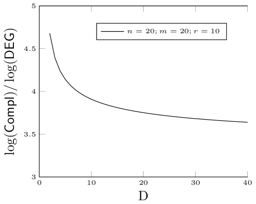
Figure 1: Numerical values of $\log(\operatorname{\sf Compl}_{\sf F_{5}})/\log(\operatorname{\sf DEG})$, for $n=m=20,r=10,k=(n-r)(m-r)$.

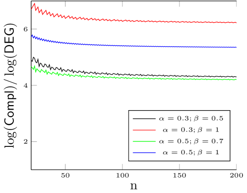
Figure 2: Numerical values of $\log(\operatorname{\sf Compl}_{\sf F_{5}})/\log(\operatorname{\sf DEG})$, for $m=\lfloor\beta n\rfloor,r=\lfloor\alpha n\rfloor-1,D=1,k=(n-r)(m-r)$.

However, there also exist families of generalized MinRank problem where the complexity bound for the Gröbner basis computation is not polynomial in the degree of ideal. For instance, taking $n=m$ and fixing the values of $r$ and $D$ yields such a family.

The experimental behavior of $\log(\operatorname{\sf Compl}_{\sf F_{5}})/\log(\operatorname{\sf DEG})$ is plotted in Figure 3. We would like to point out that this does not necessarily mean that the complexity of the Gröbner basis computation is not polynomial in the degree of the ideal. Indeed, the complexity bound $O\left(\binom{n}{r+1}\binom{m}{r+1}\binom{k+\operatorname{\mathbb{D}_{reg}}}{k}^{\omega}\right)$ is not sharp and the figure only shows that the bound is not polynomial.

The problem of showing whether the actual arithmetic complexity of the $F_{5}$ algorithm is polynomial or not in the degree of the ideal for any families of parameters of the generalized MinRank problem remains an open problem.

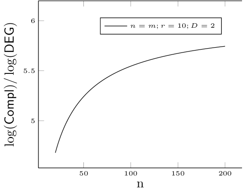
Figure 3: Numerical values of $\log(\operatorname{\sf Compl}_{\sf F_{5}})/\log(\operatorname{\sf DEG})$, for $m=\lfloor\beta n\rfloor,r=\lfloor\alpha n\rfloor-1,D=1,k=(n-r)(m-r)$.

8 Application to bi-homogeneous systems of bi-degree $(D,1)$

In this section, we show that the previous complexity analysis can be used to obtain bounds on the complexity of solving bi-homogeneous systems of bi-degree $(D,1)$ by using Gröbner bases algorithms. These structured systems can appear naturally in some applications, for instance in geometry and in optimization. Indeed the classical technique of Lagrange multipliers – when used to optimize a polynomial function under polynomial constraints – gives rise to a bi-homogeneous system of bi-degree $(D,1)$.

Bi-homogeneous polynomials are defined as follows: given two finite sets of variables $X=\{x_{0},\ldots,x_{n_{x}}\}$ and $Y=\{y_{0},\ldots,y_{n_{y}}\}$, a polynomial $f\in\mathbb{K}[X,Y]$ is called bi-homogeneous if for any $\lambda,\mu\in\mathbb{K}$, there exist $d_{x},d_{y}\in\mathbb{N}$ such that

$$f(\lambda X,\mu Y)=\lambda^{d_{x}}\mu^{d_{y}}f(X,Y).$$

The couple $(d_{x},d_{y})$ is called the bi-degree of $f$.

In this section, we focus on generic systems of $n_{x}+n_{y}$ bi-homogeneous equations of bi-degree $(D,1)$. Such systems have a finite number of solutions on the biprojective space $\mathbb{P}^{n_{x}}\times\mathbb{P}^{n_{y}}$. One way to compute them is to start by computing their projection on $\mathbb{P}^{n_{x}}$, and then lift them to $\mathbb{P}^{n_{x}}\times\mathbb{P}^{n_{y}}$ by solving linear systems (this can be done since the equations are linear with respect the variables $y_{0},\ldots,y_{n_{y}}$).

The following proposition shows that computing the projection on $\mathbb{P}^{n_{y}}$ can be computed by solving a homogeneous MinRank problem.

Proposition 3.

Let $f_{1},\ldots,f_{m}\in\mathbb{K}[X,Y]$ be a bi-homogeneous system of bi-degree $(D,1)$. If $m>n_{y}$, then $(x_{0}:\ldots:x_{n_{x}},y_{0}:\ldots:y_{n_{y}})\in\mathbb{P}^{n_{x}}\times\mathbb{P}^{n_{y}}$ is a zero of this system if and only if the matrix

$$\operatorname{jac}_{Y}(x_{0},\ldots,x_{n_{x}})=\begin{pmatrix}\frac{\partial f_{1}}{\partial y_{0}}&\dots&\frac{\partial f_{1}}{\partial y_{n_{y}}}\\ \vdots&\vdots&\vdots\\ \frac{\partial f_{m}}{\partial y_{0}}&\dots&\frac{\partial f_{m}}{\partial y_{n_{y}}}\end{pmatrix}$$

is rank defective.

Proof.

First, notice that

$$\begin{pmatrix}f_{1}\\ \vdots\\ f_{m}\end{pmatrix}=\operatorname{jac}_{Y}(x_{0},\ldots,x_{n_{x}})\cdot\begin{pmatrix}y_{0}\\ \vdots\\ y_{n_{y}}\end{pmatrix}.$$

Therefore, $(x_{0}:\ldots:x_{n_{x}},y_{0}:\ldots:y_{n_{y}})\in\mathbb{P}^{n_{x}}\times\mathbb{P}^{n_{y}}$ is a zero of the system if and only if $(y_{0},\ldots,y_{n_{y}})$ belongs to the kernel of $\operatorname{jac}_{Y}$. Since $m>n_{y}$, the number of rows is greater than or equal to the number of columns of $\operatorname{jac}_{Y}$, and hence $\operatorname{jac}_{Y}$ is rank defective. ∎

In applications, most of bi-homogeneous systems occurring are affine: A polynomial $f\in\mathbb{K}[x_{1},\ldots,x_{n_{x}},y_{1},\ldots,y_{n_{y}}]$ is called affine of bi-degree $(D,1)$ if there exists a bi-homogeneous polynomial $f^{h}\in\mathbb{K}[x_{0},\ldots,x_{n_{x}},y_{0},\ldots,y_{n_{y}}]$ of bi-degree $(D,1)$ such that

$$f(x_{1},\ldots,x_{n_{x}},y_{1},\ldots,y_{n_{y}})=f^{h}(1,x_{1},\ldots,x_{n_{x}},1,y_{1},\ldots,y_{n_{y}}).$$

This means that each monomial occurring in $f$ has bi-degree $(i,j)$ with $i\leq D$ and $j\leq 1$. Notice that the polynomial $f^{h}$ is uniquely defined and that Proposition 3 also holds in the affine context:

Proposition 4.

Let $f_{1},\ldots,f_{m}\in\mathbb{K}[x_{1},\ldots,x_{n_{x}},y_{1},\ldots,y_{n_{y}}]$ be an affine system of bi-degree $(D,1)$. If $m>n_{y}$ and $(x_{1},\ldots,x_{n_{x}},y_{1},\ldots,y_{n_{y}})\in\mathbb{K}^{n_{x}}\times\mathbb{K}^{n_{y}}$ is a zero of the system, then the $m\times(n_{y}+1)$ matrix

$$\operatorname{jac}^{a}_{Y}(x_{1},\ldots,x_{n_{x}})=\begin{pmatrix}f_{1}(x_{1},\ldots,x_{n_{x}},0,\ldots,0)&\frac{\partial f_{1}}{\partial y_{1}}&\dots&\frac{\partial f_{1}}{\partial y_{n_{y}}}\\ \vdots&\vdots&\vdots\\ f_{m}(x_{1},\ldots,x_{n_{x}},0,\ldots,0)&\frac{\partial f_{m}}{\partial y_{0}}&\dots&\frac{\partial f_{m}}{\partial y_{n_{y}}}\end{pmatrix}$$

is rank defective.

Proof.

The proof is similar to that of 3 since

$$\begin{pmatrix}f_{1}\\ \vdots\\ f_{m}\end{pmatrix}=\operatorname{jac}_{Y}^{a}(x_{1},\ldots,x_{n_{x}})\cdot\begin{pmatrix}1\\ y_{1}\\ \vdots\\ y_{n_{y}}\end{pmatrix}.$$

Therefore, if $(x_{1},\ldots,x_{n_{x}},y_{1},\ldots,y_{n_{y}})$ is a zero of the system then there is a non-zero vector in the kernel of $\operatorname{jac}_{Y}^{a}$ (however in the affine case, the converse is not true). ∎

An algebraic description of the variety $V$ of a $0$-dimensional polynomial system can be obtained by computing a rational parametrization, i.e. a polynomial $g(u)\in\mathbb{K}[u]$ and a set of rational functions $g_{1},\ldots,g_{n_{x}},h_{1},\ldots,h_{n_{y}}\in\mathbb{K}(u)$ such that

$$\begin{array}[]{c}(x_{1},\ldots,x_{n_{x}},y_{1},\ldots,y_{n_{y}})\in V\\ \Updownarrow\\ \exists u\in\mathbb{K},s.t.g(u)=0,\forall i\in\{1,\ldots,n_{x}\},x_{i}=g_{i}(u),\forall j\in\{1,\ldots,n_{y}\},y_{j}=h_{j}(u).\end{array}$$

To obtain a rational parametrization, we need a separating element: a linear form which takes different values on all points of $V$. Therefore, a rational parametrization exists only if the cardinality of the field $\mathbb{K}$ is infinite or large enough.

Algorithm 1 Rational parametrization of systems of bi-degree $(D,1)$

1:$f_{1},\ldots,f_{n_{x}+n_{y}}\in\mathbb{K}[X,Y]$ a system of affine polynomials of bi-degree $(D,1)$ such that the ideal they generate is radical and $0$-dimensional;
$(\alpha_{1},\ldots,\alpha_{n_{x}-1})\in\mathbb{K}^{n_{x}-1}$;
a full rank matrix $M=(m_{i,j})\in\mathbb{K}^{ny\times(n_{x}+n_{y})}$.

2:Returns a rational parametrization of the variety of the system or “fail”.

3:Compute for each $i\in\{1,\ldots,n_{x}+n_{y}\}$,

$$\widetilde{f_{i}}(x_{1},\ldots,x_{n_{x}-1},u,y_{1},\ldots,y_{n_{y}})=f_{i}(x_{1},\ldots,x_{n_{x}-1},u-\displaystyle\sum_{\ell=1}^{{n_{x}}-1}\alpha_{\ell}x_{\ell},y_{1},\ldots,y_{n_{y}}).$$

4:Compute the matrix $\operatorname{jac}^{a}_{Y}(\widetilde{f_{1}},\ldots,\widetilde{f_{n_{x}+n_{y}}})$.

5:Compute a lex Gröbner basis $G$ of the ideal $I\subset\mathbb{K}[x_{1},\ldots,x_{n_{x}-1},u]$ generated by the maximal minors of the matrix $\operatorname{jac}^{a}_{Y}(\widetilde{f_{1}},\ldots,\widetilde{f_{n_{x}+n_{y}}})$. If the Gröbner basis has the following shape (the shape position):

$$\begin{array}[]{r}x_{1}-g_{1}(u)\\ x_{2}-g_{2}(u)\\ \vdots\\ x_{n_{x}-1}-g_{n_{x}-1}(u)\\ g(u),\end{array}$$

then continue to Step 4, else return “fail”.

6:Using $M$, compute a linear combination of the polynomials of the system evaluated at $(g_{1}(u),\ldots,g_{n_{x}-1}(u))$:

$$\begin{pmatrix}\widehat{f_{1}}(y_{1},\ldots,y_{n_{y}},u)\\ \vdots\\ \widehat{f_{n_{y}}}(y_{1},\ldots,y_{n_{y}},u)\end{pmatrix}=M\cdot\begin{pmatrix}\widetilde{f_{1}}(g_{1}(u),\ldots,g_{n_{x}-1}(u),u,y_{1},\ldots,y_{n_{y}})\mod g(u)\\ \vdots\\ \widetilde{f_{n_{x}+n_{y}}}(g_{1}(u),\ldots,g_{n_{x}-1}(u),u,y_{1},\ldots,y_{n_{y}})\mod g(u)\end{pmatrix}$$

7:If the linear system $\widehat{f_{1}}=\ldots=\widehat{f_{n_{y}}}=0$ has rank $n_{y}$ (as a linear system in $\mathbb{K}(u)[Y]$ where the variables are $y_{1},\ldots,y_{n_{y}}$), continue to Step 6, else return “fail”.

8:Using Cramer’s rule, solve the system $\widehat{f_{1}}=\ldots=\widehat{f_{n_{y}}}=0$ as a linear system in $\mathbb{K}(u)[Y]$. This yields rational functions $h_{i}(u)\in\mathbb{K}(u)$ such that, for $i\in\{1,\ldots,n_{y}\}$, $y_{i}-h_{i}(u)=0$.

9:Return the rational parametrization

$$\begin{array}[]{cc}g(u)=0&\\ x_{1}=g_{1}(u)&y_{1}=h_{1}(u)\\ \vdots&\vdots\\ x_{n_{x}-1}=g_{n_{x}-1}(u)&y_{n_{y}-1}=h_{n_{y}-1}(u)\\ x_{n_{x}}=u-\displaystyle\sum_{\ell=1}^{{n_{x}}-1}\alpha_{\ell}g_{\ell}(u)&y_{n_{y}}=h_{n_{y}}(u)\end{array}$$

Under the assumption that the field $\mathbb{K}$ is sufficiently large, Algorithm 1 uses the property described in Proposition 4 to find a rational parametrization of the zeroes of a radical and $0$-dimensional system of $n_{x}+n_{y}$ affine polynomials of bi-degree $(D,1)$. The algorithm proceeds by computing first a rational parametrization of the projection of the zero set on $\mathbb{K}^{n_{x}}$. This is done by computing a lexicographical Gröbner basis of a Generalized MinRank Problem. Then this parametrization is lifted to the whole space by solving a linear system (this can be done since the equations are linear with respect to the variables $y_{1},\ldots,y_{n_{y}}$).

The success of Algorithm 1 depends on the choice of the parameters $\alpha$ (a linear change of coordinates such that $x_{n}$ is a separating element) and $M$. However, as we will see in Theorem 6, if the cardinality of $\mathbb{K}$ is infinite or large enough, then almost all choices of $\alpha$ and $M$ are good. Therefore, these parameters can be chosen at random. If Algorithm 1 unluckily fails, then it can be restarted with the same algebraic system and different values of $\alpha$ and $M$.

We now prove that the complexity of Algorithm 1 is bounded by the complexity of the underlying generalized MinRank problem and that most choices of $(\alpha_{1},\ldots,\alpha_{n_{x}-1})$ and $M$ do not fail.

Theorem 6.

Let $f_{1},\ldots,f_{n_{x}+n_{y}}\in\mathbb{K}[X,Y]$ be an affine system of bi-degree $(D,1)$ such that the ideal $\langle f_{1},\ldots,f_{n_{x}+n_{y}}\rangle$ is radical and $0$-dimensional. Then there exists non-identically null polynomials $h_{1}\in\mathbb{K}[z_{1},\ldots,z_{n_{x}-1}]$ and $h_{2}\in\mathbb{K}[z_{1,1},\ldots,z_{n_{y},n_{x}+n_{y}}]$ such that, for any choice of $(\alpha_{1},\ldots,\alpha_{n_{x}-1})$ and $M=(m_{i,j})\in\mathbb{K}^{n_{y}\times(n_{x}+n_{y})}$ verifying:

• the matrix $\operatorname{jac}^{a}_{Y}(\widetilde{f_{1}},\ldots,\widetilde{f_{n_{x}+n_{y}}})$ verifies the conditions of Theorem 5;

• $h_{1}(\alpha_{1},\ldots,\alpha_{n_{x}-1})h_{2}(m_{1,1},\ldots,m_{n_{y},n_{x}+n_{y}})\neq 0$,

Algorithm 1 returns a rational parametrization of the variety of the system and its complexity is upper bounded by

$$O\left(\binom{n_{x}+n_{y}}{n_{x}-1}\binom{D(n_{x}+n_{y})+1}{n_{x}}^{\omega}+n_{x}\left(D^{n_{x}}\binom{n_{x}+n_{y}}{n_{x}}\right)^{3}\right).$$

Proof.

In this proof, $\widetilde{O}()$ stands for the soft-Oh notation: if $f$ and $g$ are positive functions, $f=\widetilde{O}(g)$ means that there exists $k\in\mathbb{N}$ such that $f=O(g\cdot\log^{k}(g))$. Let $I$ denote the ideal generated by $f_{1},\ldots,f_{n_{x}+n_{y}}$. According to [29, 4], for any radical $0$-dimensional ideal, there exists a polynomial $h_{1}$ such that if $h_{1}(\alpha_{1},\ldots,\alpha_{n_{x}-1})\neq 0$, then the system is in shape position after the change of coordinates

$$x_{n_{x}}\mapsto x_{n_{x}}-\sum_{\ell=1}^{n_{x}-1}\alpha_{\ell}x_{\ell}.$$

The polynomial $h_{2}$ is chosen such that if $h_{2}(m_{i,j})\neq 0$, then the linear system $\widehat{f_{1}}=\dots=\widehat{f_{n_{y}}}=0$ in $\mathbb{K}(u)[Y]$ has rank exactly $n_{y}$. Consider now the following linear system (where the variables are $y_{1},\ldots,y_{n_{y}}$):

$$\begin{pmatrix}z_{1,1}&\dots&z_{1,n_{x}+n_{y}}\\ \vdots&\vdots&\vdots\\ z_{n_{y},1}&\dots&z_{n_{y},n_{x}+n_{y}}\end{pmatrix}\cdot\begin{pmatrix}\widetilde{f_{1}}(g_{1}(u),\ldots,g_{n_{x}-1}(u),u,y_{1},\ldots,y_{n_{y}})\mod g(u)\\ \vdots\\ \widetilde{f_{n_{x}+n_{y}}}(g_{1}(u),\ldots,g_{n_{x}-1}(u),u,y_{1},\ldots,y_{n_{y}})\mod g(u)\end{pmatrix}=0.$$

Its determinant (which lies in $\mathbb{K}[z_{1,1},\ldots,z_{n_{y},n_{x}+n_{y}},u]$) is not zero since the ideal generated by the input system $(f_{1},\ldots,f_{n_{x}+n_{y}})$ is $0$-dimensional and proper. By considering this determinant as a polynomial in $\mathbb{K}[z_{1,1},\ldots,z_{n_{y},n_{x}+n_{y}}][u]$, the polynomial $h_{2}\in\mathbb{K}[z_{1,1},\ldots,z_{n_{y},n_{x}+n_{y}}]$ is chosen as a non-zero coefficient of a term $u^{\beta}$. Consequently, the algorithm does not fail if $h_{1}(\alpha_{1},\ldots,\alpha_{n_{x}-1})\neq 0$ and $h_{2}(m_{i,j})\neq 0$.

Now we proceed with the complexity analysis:

• the complexity of the substitution step to compute the polynomials $\widetilde{f_{i}}$ is upper bounded by $\widetilde{O}((n_{x}+n_{y})Dn_{x}n_{y})$.

• By Theorem 5, the complexity of the Gröbner basis computation is upper bounded by

  $$O\left(\binom{n_{x}+n_{y}}{n_{x}-1}\binom{D(n_{x}+n_{y})+1}{n_{x}}^{\omega}+n_{x}\left(\operatorname{\sf DEG}(I)\right)^{3}\right).$$

• Since $\deg(g_{n_{x}})\leq\operatorname{\sf DEG}(I)$, a monomial $u^{n_{x}}\prod_{i=1}^{n_{x}-1}x_{i}^{\alpha_{i}}$ of degree $D$ can be evaluated in the univariate polynomials $(g_{1}(u),\dots,g_{n_{x}-1}(u))$ modulo $g(u)$ in complexity $\widetilde{O}(D\operatorname{\sf DEG}(I))$ by using a subproduct tree [7], quasi-linear multiplication of univariate polynomials and quasi-linear modular reduction. Since there are at most $(n_{x}+n_{y})(n_{y}+1)\binom{n_{x}+D}{n_{x}}$ such monomials in the system $f_{1},\ldots,f_{n_{x}+n_{y}}$, the Step 4 of the Algorithm needs at most

  $$\widetilde{O}\left((n_{x}+n_{y})n_{y}\binom{n_{x}+D}{n_{x}}D\operatorname{\sf DEG}(I)\right)$$

  arithmetic operations in $\mathbb{K}$.
  Notice that $n_{x}+n_{y}\leq\binom{n_{x}+n_{y}}{n_{x}-1}$ and $\operatorname{\sf DEG}(I)\leq\binom{D(n_{x}+n_{y})+1}{n_{x}}$.

  • If $D\geq 2$: for any $a,b,c\in\mathbb{N}$ such that $b<a$, $\binom{a}{b}c\leq\binom{a+c}{b}$. Therefore, $Dn_{y}\binom{n_{x}+D}{n_{x}}\leq\binom{n_{x}+n_{y}+2D}{n_{x}}$. Also, notice that, for $D\geq 2$ and for any $n_{x},n_{y}$ such that $n_{x}n_{y}>1$, $n_{x}+n_{y}+2D\leq D(n_{x}+n_{y})+1$. Therefore,

    $$\widetilde{O}\left((n_{x}+n_{y})n_{y}\binom{n_{x}+D}{n_{x}}D\operatorname{\sf DEG}(I)\right)\leq\widetilde{O}\left(\binom{n_{x}+n_{y}}{n_{x}-1}\binom{D(n_{x}+n_{y})+1}{n_{x}}^{2}\right).$$

  • If $D=1$: $(n_{x}+n_{y})n_{y}\binom{n_{x}+1}{n_{x}}=(n_{x}+n_{y})n_{y}n_{x}$ is bounded by $\binom{n_{x}+n_{y}}{n_{x}-1}\binom{(n_{x}+n_{y})+1}{n_{x}}$.

  Therefore, the complexity of the Step 4 of Algorithm 1 is upper bounded by the complexity of the Gröbner basis computation: $O\left(\binom{n_{x}+n_{y}}{n_{x}-1}\binom{D(n_{x}+n_{y})+1}{n_{x}}^{\omega}\right).$

• To solve the linear system by using Cramer’s rule, we need to compute $n_{x}+1$ determinants of $(n_{x}\times n_{x})$-matrices whose entries are univariate polynomials of degree $D$. This can be achieved by using a fast evaluation-interpolation strategy with complexity $\widetilde{O}\left(Dn_{x}^{\omega+1}\right)$ (since multi-set evaluation and interpolation of univariate polynomials can be done in quasi-linear time, see e.g. [7]).

Since $\operatorname{\sf DEG}(I)$ is bounded by $D^{n_{x}}\binom{n_{x}+n_{y}}{n_{x}}$, the sum of all these complexities is upper bounded by

$$O\left(\binom{n_{x}+n_{y}}{n_{x}-1}\binom{D(n_{x}+n_{y})+1}{n_{x}}^{\omega}+n_{x}\left(D^{n_{x}}\binom{n_{x}+n_{y}}{n_{x}}\right)^{3}\right).$$

∎

Remark 4.

According to [19, Lemma 15] and [19, Lemma 16], if $D=1$, there exists a non-empty Zariski open subset $O_{1}$ of the set of systems of bi-degree $(1,1)$, such that any system $(f_{1},\ldots,f_{n_{x}+n_{y}})\in O_{1}$ is $0$-dimensional and radical. This statement also holds for systems of bi-degree $(D,1)$ with $D\in\mathbb{N}$, and the proof is similar.

Acknowledgments

This work was supported in part by the HPAC grant and the GeoLMI grant (ANR 2011 BS03 011 06) of the French National Research Agency. The second author is member of the Institut Universitaire de France. We wish to thank anonymous referees for their comments and suggestions.

References

• [1] B. Bank, M. Giusti, J. Heintz, M. Safey El Din, and E. Schost. On the geometry of polar varieties. Applicable Algebra in Engineering, Communication and Computing, 21(1):33–83, 2010.
• [2] M. Bardet. Étude des systèmes algébriques surdéterminés. Applications aux codes correcteurs et à la cryptographie. PhD thesis, Université Paris 6, 2004.
• [3] M. Bardet, J.-C. Faugère, and B. Salvy. Asymptotic expansion of the degree of regularity for semi-regular systems of equations. In Effective Methods in Algebraic Geometry (MEGA), pages 71–74, 2004.
• [4] E. Becker, T. Mora, M. Marinari, and C. Traverso. The shape of the shape lemma. In Proceedings of the International Symposium on Symbolic and Algebraic Computation, ISSAC ’94, pages 129–133, New York, NY, USA, 1994. ACM.
• [5] L. Bettale, J.-C. Faugère, and L. Perret. Cryptanalysis of HFE, Multi-HFE and Variants for Odd and Even Characteristic. Designs, Codes and Cryptography, pages 1–52, 2012. accepted.
• [6] W. Bosma, J. Cannon, and C. Playoust. The Magma algebra system. I. The user language. Journal of Symbolic Computation, 24(3–4):235–265, 1997.
• [7] A. Bostan and É. Schost. Polynomial evaluation and interpolation on special sets of points. Journal of Complexity, 21(4):420–446, 2005.
• [8] J. F. Buss, G. S. Frandsen, and J. Shallit. The computational complexity of some problems of linear algebra. Journal of Computer and System Sciences, 58(3):572–596, 1999.
• [9] A. Conca and J. Herzog. On the Hilbert function of determinantal rings and their canonical module. Proceedings of the American Mathematical Society, 122(3):677–681, 1994.
• [10] N. Courtois. Efficient zero-knowledge authentication based on a linear algebra problem MinRank. In Advances in Cryptology - ASIACRYPT 2001, volume 2248 of LNCS, pages 402–421. Springer, 2001.
• [11] D. Cox, J. Little, and D. O’Shea. Ideals, Varieties and Algorithms. Springer, 3rd edition, 1997.
• [12] D. Eisenbud. Commutative Algebra with a View Toward Algebraic Geometry. Springer, 1995.
• [13] J.-C. Faugère. A new efficient algorithm for computing Gröbner bases (F4). Journal of Pure and Applied Algebra, 139(1–3):61–88, 1999.
• [14] J.-C. Faugère. A new efficient algorithm for computing Gröbner bases without reductions to zero (F5). In T. Mora, editor, Proceedings of the 2002 International Symposium on Symbolic and Algebraic Computation (ISSAC), pages 75–83. ACM Press, 2002.
• [15] J.-C. Faugère, P. Gianni, D. Lazard, and T. Mora. Efficient computation of zero-dimensional Gröbner bases by change of ordering. Journal of Symbolic Computation, 16(4):329–344, 1993.
• [16] J.-C. Faugère, F. Lévy-dit-Vehel, and L. Perret. Cryptanalysis of MinRank. In Advances in Cryptology - CRYPTO 2008, volume 5157 of LNCS, pages 280–296. Springer, 2008.
• [17] J.-C. Faugère and C. Mou. Fast algorithm for change of ordering of zero-dimensional Gröbner bases with sparse multiplication matrices. In ISSAC ’11: Proceedings of the 2011 International Symposium on Symbolic and Algebraic Computation, ISSAC ’11, pages 1–8. ACM, 2011.
• [18] J.-C. Faugère, M. Safey El Din, and P.-J. Spaenlehauer. Computing loci of rank defects of linear matrices using Gröbner bases and applications to cryptology. In S. M. Watt, editor, Proceedings of the 2010 International Symposium on Symbolic and Algebraic Computation (ISSAC 2010), pages 257–264, 2010.
• [19] J.-C. Faugère, M. Safey El Din, and P.-J. Spaenlehauer. Gröbner bases of bihomogeneous ideals generated by polynomials of bidegree (1,1): Algorithms and complexity. Journal Of Symbolic Computation, 46(4):406–437, 2011.
• [20] R. Fröberg. An inequality for Hilbert series of graded algebras. Mathematica Scandinavica, 56:117–144, 1985.
• [21] W. Fulton. Intersection Theory. Springer, 2nd edition, 1997.
• [22] M. Giusti, G. Lecerf, and B. Salvy. A Gröbner free alternative for polynomial system solving. Journal of Complexity, 17(1):154–211, 2001.
• [23] G. Greuel, C. Lossen, and E. Shustin. Introduction to singularities and deformations. Springer, 2007.
• [24] A. Greuet, F. Guo, M. Safey El Din, and L. Zhi. Global optimization of polynomials restricted to a smooth variety using sums of squares. Journal of Symbolic Computation, 47(5):503–518, 2012.
• [25] M. Hochster and J. A. Eagon. A class of perfect determinantal ideals. Bulletin of the American Mathematical Society, 76(5):1026–1029, 1970.
• [26] M. Hochster and J. A. Eagon. Cohen-Macaulay rings, invariant theory, and the generic perfection of determinantal loci. American Journal of Mathematics, 93(4):1020–1058, 1971.
• [27] H. Hong and M. S. E. Din. Variant quantifier elimination. J. Symb. Comput., 47(7):883–901, 2012.
• [28] A. Kipnis and A. Shamir. Cryptanalysis of the HFE public key cryptosystem by relinearization. In Advances in Cryptology - CRYPTO’ 99, volume 1666 of LNCS, pages 19–30. Springer, 1999.
• [29] Y. N. Lakshman. On the complexity of computing a Gröbner basis for the radical of a zero dimensional ideal. In Proceedings of the twenty-second annual ACM Symposium on Theory Of computing, STOC ’90, pages 555–563, New York, NY, USA, 1990. ACM.
• [30] D. Lazard. Gröbner bases, Gaussian elimination and resolution of systems of algebraic equations. In Computer Algebra, EUROCAL’83, volume 162 of LNCS, pages 146–156. Springer, 1983.
• [31] I. G. Macdonald, J. Pach, and T. Theobald. Common tangents to four unit balls in r 3. Discrete & Computational Geometry, 26(1):1–17, 2001.
• [32] E. Miller and B. Sturmfels. Combinatorial commutative algebra, volume 227. Springer Verlag, 2005.
• [33] A. Ourivski and T. Johansson. New technique for decoding codes in the rank metric and its cryptography applications. Problems of Information Transmission, 38(3):237–246, 2002.
• [34] M. Safey El Din and E. Schost. Polar varieties and computation of one point in each connected component of a smooth real algebraic set. In Proceedings of the 2003 international symposium on Symbolic and algebraic computation, pages 224–231. ACM, 2003.
• [35] F. Sottile. From enumerative geometry to solving systems of polynomial equations. Computations in algebraic geometry with Macaulay, 2:101–129, 2002.
• [36] F. Sottile. Enumerative real algebraic geometry. Algorithmic and Quantitative Real Algebraic Geometry, pages 139–179, 2003.
• [37] A. Storjohann. Algorithms for Matrix Canonical Forms. PhD thesis, University of Waterloo, 2000.
• [38] J. Verschelde. Polynomial homotopies for dense, sparse and determinantal systems, 1999.
• [39] V. Williams. Breaking the Coppersmith-Winograd barrier, 2011.