Geometry of the adiabatic theorem

Abstract

We present a simple and pedagogical derivation of the quantum adiabatic theorem for two level systems (a single qubit) based on geometrical structures of quantum mechanics developed by Anandan and Aharonov, among others. We have chosen to use only the minimum geometric structure needed for an understanding of the adiabatic theorem for this case.

I Introduction

The quantum mechanical adiabatic theorem is one of the most important and fruitful tools of quantum physics. It was first stated in 1928 by Born and Fock Born and Fock (1928) and set in a more rigorous mathematical foundation in 1950 by Kato Kato (1950). In the mid-eighties, it was linked in a new and fundamental way with a more geometrical view of quantum mechanics by the so called Berry’s phase or geometric phase Berry (1984); Aharonov and Anandan (1987).

More recently, it has received a renewal of interest because of the advent of quantum information theory and in particular, the quantum adiabatic computation model Farhi et al. (2000); Aharonov et al. (2004). In fact, some authors have questioned the theorem and have tried to look for a more precise statement and conditions for its consistency and validity Marzlin and Sanders (2004); Wu and Yang (2005); Tong et al. (2005); Ma et al. (2006); Wei and Ying (2007); Amin (2009); Boixo and Somma (2010); Frasca (2011); Rigolin and Ortiz (2011).

Though the theorem can be stated and understood quite easily and it is, in fact, routinely discussed in undergraduate textbooks Griffiths (2005); Messiah (1999), we believe that the reason why it works though, is less known. It can be simply stated as saying that under a certain special context, if the state of a quantum mechanical system is an eigenstate of its hamiltonian, it will remain as such. The special context means that the time-dependent hamiltonian must change slowly in some sense (adiabaticity) if the spectrum obeys some technical conditions. Stated in this manner, one can say it is a reasonably intuitive assertion and can be traced back to its correspondent classical theorem on adiabatic invariants Kasuga (1961). Yet, the proofs available to students such as in Messiah (1999) are technically difficult and for this reason they may not be very enlightening for the average student.

We shall discuss the reasons for the validity of the theorem for two-state systems in a setting inspired by the geometrical treatment of quantum mechanics given by Anandan and Aharonov Anandan and Aharonov (1990). In the next Section, we review the geometry of quantum evolution for finite dimensional systems and in particular, for two-level systems (which in modern quantum information theory are called qubits) and use this to discuss the quantum adiabatic theorem in a very clean and pedagogical geometric setting which we believe improves the physical understanding of this important theorem for students of Physics and even for specialists. In Section III we conclude with some closing remarks.

II The Geometry of Quantum Evolution

Let $W^{n+1}$ be a $(n+1)$-dimensional Hilbert space together with its dual $\overline{W}^{n+1}$ and let $\{|u_{\sigma}\rangle\}$ $(\sigma=0,1,...,n)$ also be an arbitrary basis for $W^{n+1}.$ An hermitean inner product may be introduced by an anti-linear mapping ${\dagger}:W^{n+1}\longrightarrow\overline{W}^{n+1}$ (where ${\dagger}$ is the familiar “dagger” operation). Indeed, the inner product between two arbitrary states $|\psi\rangle$ and $|\varphi\rangle$ can now be defined as

$$(|\psi\rangle,|\varphi\rangle)=|\psi\rangle\left({}^{\dagger}|\varphi\rangle\right)=\langle\psi|\varphi\rangle.$$

Thus, an arbitrary normalized ket $|\psi\rangle$ expanded in such a basis can be represented by a complex $(n+1)$-column matrix:

$$|\psi\rangle=\sum\limits_{\sigma}|u_{\sigma}\rangle\psi^{\sigma}\equiv(\begin{array}[c]{cccc}\psi_{0}&\psi_{1}&...&\psi_{n}\end{array})^{\intercal},\quad\text{with}\quad\sum\limits_{\sigma}\overline{\psi}_{\sigma}\psi^{\sigma}=1.$$ (1)

Writing the complex amplitudes as $\psi^{\sigma}=x^{\sigma}+iy^{\sigma}$ one can easily see that the set of normalized states can be identified with a $(2n+1)$-dimensional sphere $S^{2n+1}$ contained in $W^{n+1}$. Since two state vectors that differ by a complex phase cannot be physically distinguished by any means, it is convenient to define the true physical space of states as the above set of normalized states modulo the equivalence relation in $S^{2n+1}$ defined in the following way: We say that $|\psi\rangle$ is equivalent to $|\varphi\rangle$ if and only if there is a real number $\theta$ such that $|\psi\rangle=e^{i\theta}|\varphi\rangle.$ The space of rays defined above is also known as the $n$-dimensional (complex) projective space $\mathbb{CP}(n)$. A standard complex coordinate system for $\mathbb{CP}(n)$ is provided by $n$ complex numbers $\xi^{i}=\psi^{i}\diagup\psi^{0}$ ($i=1,...,n$) for those points where $\psi^{0}\neq 0$. In the $n=1$ case we have a single qubit described by a single complex coordinate $\xi$. In this case, $\mathbb{CP}(1)$ is topologically equivalent to a two-dimensional sphere and the stereographic projection map shows explicitly

$$\xi=\tan(\theta/2)e^{i\varphi}$$ (2)

(see the figure below) that $\mathbb{CP}(1)$ can be seen as the complex plane “plus” a point at “infinity”.

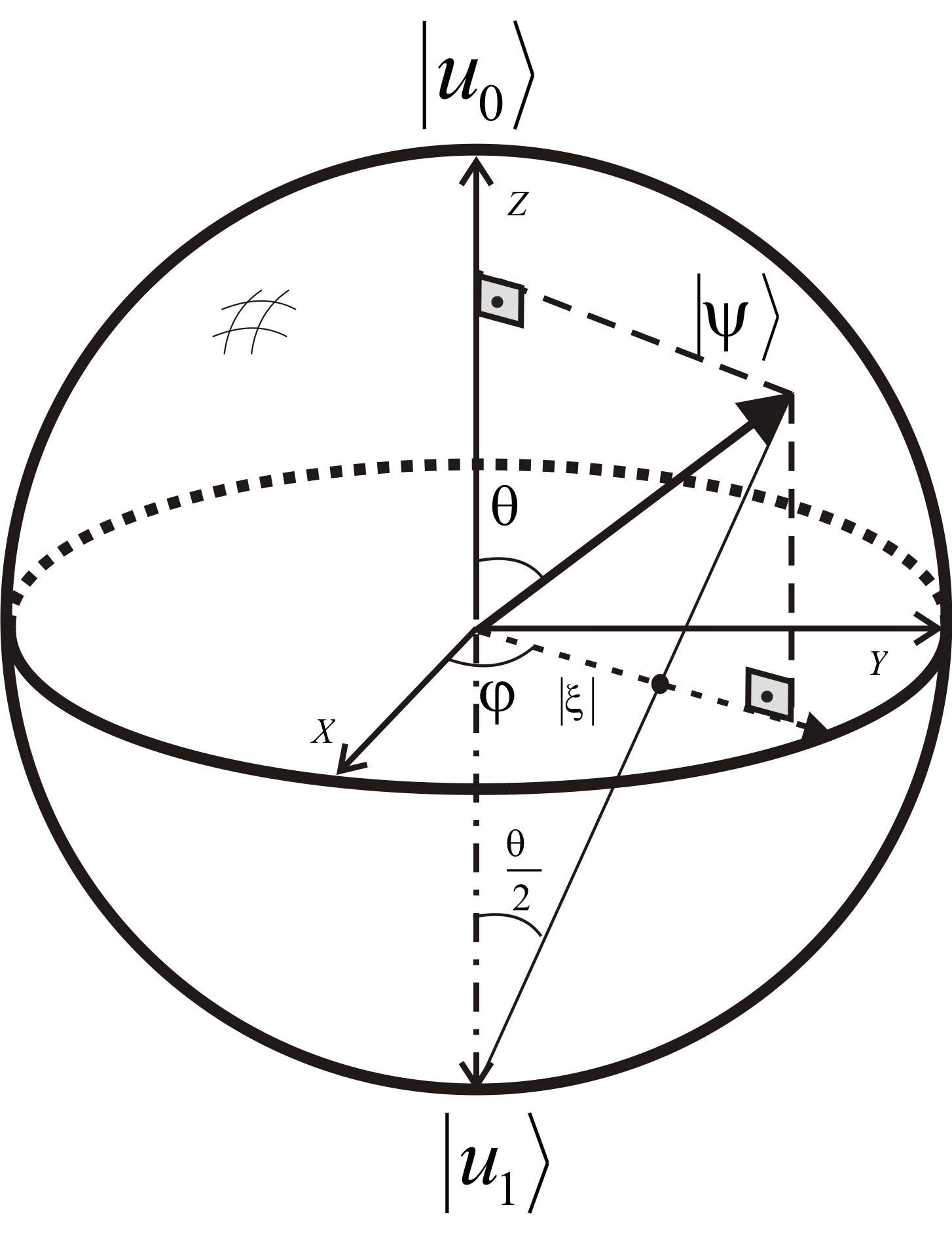
Figure 1: Stereographic projection.

This description provides us with the so called Bloch sphere (or Riemann sphere) with standard coordinates. Thus, any physical state can be expressed as a normalized state represented as a point on the Bloch sphere in the following standard form

$$|\psi\rangle=|\theta,\varphi\rangle=\cos\left(\theta/2\right)|u_{0}\rangle+e^{i\varphi}\sin\left(\theta/2\right)|u_{1}\rangle,$$ (3)

where one can easily see that antipodal points in the Bloch sphere represent orthogonal state vectors. A natural metric $\mathbb{CP}(n)$ can be defined in the following way: Let points $P_{0}$ and $P_{1}$ $\in$ $\mathbb{CP}(n)$ be projections respectively from two infinitesimally nearby normalized state vectors $|\psi\rangle$ and $|\psi+d\psi\rangle$. It is then natural to define the squared distance between $P_{0}$ and $P_{1}$ as the projection of $|d\psi\rangle$ in the “orthogonal direction” of $|\psi\rangle$, that is, the projection given by the projection operator $\hat{\pi}_{|\psi\rangle}^{\perp}=\hat{I}-|\psi\rangle\langle\psi|$ as shown in FIG. 2. It is then easy to see that (by the idempotence of $\hat{\pi}_{|\psi\rangle}^{\perp}$)

$$ds^{2}(\mathbb{CP}(n))=\left|\langle d\psi|\hat{\pi}_{|\psi\rangle}^{\perp}|d\psi\rangle\right|^{2}=\langle d\psi|d\psi\rangle-\langle d\psi|\psi\rangle\langle\psi|d\psi\rangle.$$ (4)

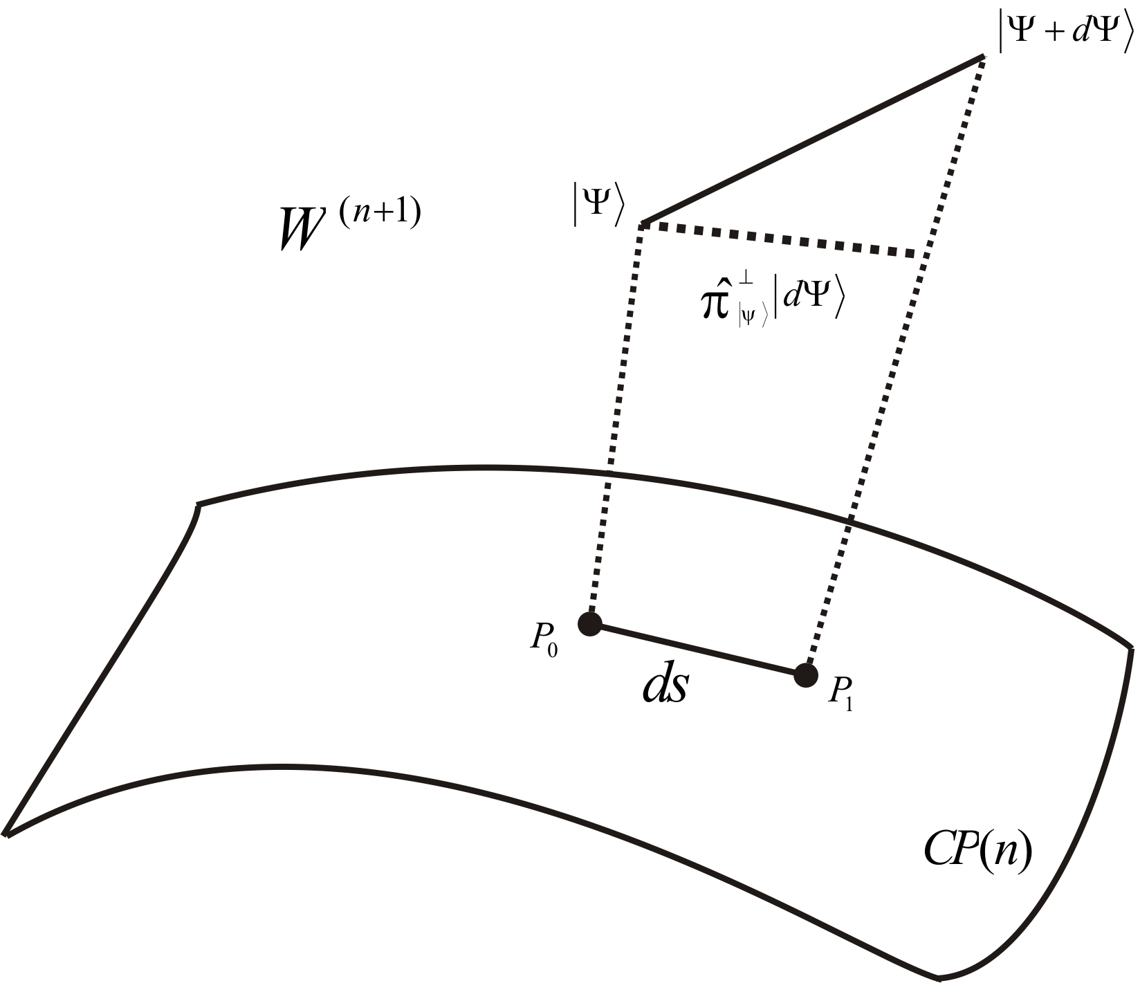
Figure 2: Pictorial representation of the geometry in $\mathbb{CP}(n))$

Let $|\psi(t)\rangle$ be the curve of normalized state vectors in $W^{n+1}$ given by the unitary evolution generated by an hamiltonian $\hat{H}$. The Schrödinger equation implies a relation between $|\psi(t)\rangle$ and $|\psi(t+dt)\rangle$ given by:

$$|d\psi\rangle=|\psi(t+dt)\rangle-|\psi(t)\rangle=-i\hat{H}|\psi(t)\rangle dt,$$ (5)

for the sake of simplification we have used and henceforth will be assuming $\hslash=1$ units. The above equation together with (4) gives us the squared distance between two infinitesimally nearby projection of state vectors connected by the unitary evolution over $\mathbb{CP}(n)$:

$$ds^{2}(\mathbb{CP}(n))=\left[\langle\psi(t)|\hat{H}^{2}|\psi(t)\rangle-(\langle\psi(t)|\hat{H}|\psi(t)\rangle)^{2}\right]dt^{2}=\left(\delta_{|\psi(t)\rangle}^{2}E\right)dt^{2}.$$ (6)

In particular, for a single qubit, one can write the metric over the $\mathbb{CP}(1)$ sphere by (3) as

$$ds^{2}=\frac{1}{4}(d\theta^{2}+\sin^{2}\theta d\varphi^{2})$$ (7)

where we can immediately identify the Bloch sphere as a $2D$ sphere with radius $r=1/2$. Note that some authors define the Bloch sphere as a unit radius sphere. Our choice seems more natural to us because of the above geometrical construction and also in order to identify the Bloch sphere with the so called Riemann sphere.

II.1 The time-energy uncertainty relation

Equation (6) leads to a very elegant relation between the speed of the projection over $\mathbb{CP}(n)$ and the instantaneous energy uncertainty Anandan and Aharonov (1990).

$$\frac{ds}{dt}=\delta E(t).$$ (8)

The above equation contains in itself the seeds of both a beautiful geometric formulation of the time-energy uncertainty relation and as well as the adiabatic theorem. Indeed, for the latter, it is quite clear that if a state is initially (let us say for $t=0$) an energy eigenstate, then one has $\delta E(0)=0$ and the instantaneous speed must then also be null. If one moves the state very slowly around $\mathbb{CP}(n)$, such that $\frac{ds}{dt}\approx 0$ then one should have in a self consistent way that $\delta E(t)\approx 0$ for all $t$. But this means that the state must remain an eigenstate for all $t$, which is exactly a statement of the adiabatic theorem and we shall discuss this issue further in the next Subsection.

Before that, let us close this Subsection by observing how equation (8) also implies a geometric version of the time-energy uncertainty relation due to Anandan and Aharonov. Let us assume at first that the system consists only of a single qubit. Let $P_{0}$ and $P_{1}$ be two distinct points on Bloch sphere located on an arbitrary path driven by a time dependent hamiltonian $\hat{H}(t)$ at instants respectively $t_{0}$ and $t_{1}$. One can define the time average of the energy uncertainty $\overline{\delta E}$ between $t_{0}$ and $t_{1}$ as

$$\overline{\delta E}=\frac{1}{\Delta t}\int_{t_{0}}^{t_{1}}\delta E(t)dt\qquad\text{with}\qquad\Delta t=t_{1}-t_{0}$$ (9)

With this definition and from (8) it is easy to see that

$$\Delta s=\overline{\delta E}\Delta t$$ (10)

Now to derive the time-energy uncertainty relation, we may borrow an elementary argument from quantum mechanics updated with a more modern flavor from quantum information. In fact, given a particular state (an arbitrary point in Bloch sphere) one can physically distinguish it from another state if and only if this second point is orthogonal to it (its antipodal point on the sphere). In fact, the indistinguishability of non-orthogonal state vectors is a basic result in quantum information together with the no-cloning theorem, for instance. The indistinguishability of non-orthogonal states means that one party (let us say Alice) cannot reliably transmit information to a second party (call him Bob) from a common agreed upon alphabet of non-orthogonal states because these states cannot be simultaneously eigenstates of commuting observables. For two-level systems, this means that for the two points $P_{0}$ and $P_{1}$ to be physically distinguished, their minimum distance must necessarily be the half length of a great circle of the Bloch sphere, which is clearly $\pi/2$. So we may write the time-energy uncertainty relation as

$$\overline{\delta E}\Delta t\geqslant\pi/2$$ (11)

Notice that the above inequality differs from the usual text-book relation by a factor of $\pi$. This is a very different mathematical picture than the one exhibited by the celebrated Heisenberg uncertainty relation for position and momentum. But this is expected because in non-relativistic mechanics, time is an external parameter and not an observable as it happens to be the case for the position operator. In fact, some authors refer to the time $\Delta t$ in the inequality above as passage time Brody (2003).

II.2 The Adiabatic Theorem in $\mathbb{CP}(1)$

By using (1), we can write the Schrödinger equation explicitly in coordinates as

$${\displaystyle\sum\limits_{\nu}}H_{\nu}^{\mu}\psi^{\nu}=i\dot{\psi}^{\mu}$$ (12)

For a two-level system (a single qubit) one can write

$$\left\{\begin{array}[c]{c}H_{0}^{0}\psi^{0}+H_{1}^{0}\psi^{1}=i\dot{\psi}^{0}\\ H_{0}^{1}\psi^{0}+H_{1}^{1}\psi^{1}=i\dot{\psi}^{1}\end{array}\right.\qquad\text{with\qquad}\hat{H}(t)=\left(\begin{array}[c]{cc}H_{0}^{0}(t)&H_{1}^{0}(t)\\ H_{0}^{1}(t)&H_{1}^{1}(t)\end{array}\right)$$ (13)

We can project this equation of motion over the sphere $\mathbb{CP}(1)$ (by using the complex projective coordinate $\xi=\psi^{1}\diagup\psi^{0}$) as a single  complex-valued first order differential equation over the space of rays:

$$\dot{\xi}=i\left[\xi\left(H_{0}^{0}-H_{1}^{1}\right)+\xi^{2}H_{1}^{0}-H_{0}^{1}\right]$$ (14)

We find it useful to define the following real functions of time in terms of the matrix elements of the hamiltonian:

$$\Omega(t)=H_{0}^{0}-H_{1}^{1}\qquad\text{and\qquad}H_{1}^{0}=\overline{H}_{0}^{1}=R(t)e^{-i\lambda(t)}$$ (15)

Note that, though a generic $2\times 2$ hermitian matrix has four independent matrix elements, the projection of the motion on $\mathbb{CP}(1)$ needs at most three arbitrary time functions. This is because the projection of the motion on ray space is invariant under a translation-by-identity transformation as $\hat{H}\rightarrow\hat{H}+f(t)\hat{I}$ since this would modify only the overall phase of the state vector but clearly leaves unchanged the value of $\Omega$. With these three defined parameters together with the stereographic coordinates provided by (2) we arrive at the following pair of coupled non-autonomous ODE’s over the Bloch sphere:

$$\left\{\begin{array}[c]{c}\dot{\theta}=-2R(t)\sin\left(\varphi-\lambda(t)\right)\\ \dot{\varphi}=\Omega(t)-2R(t)\cot\theta\cos\left(\varphi-\lambda(t)\right)\end{array}\right.$$ (16)

For an autonomous system, taking $\left\{\left|u_{0}\right\rangle,\left|u_{1}\right\rangle\right\}$ as the energy eigenstates $\hat{H}\left|u_{\sigma}\right\rangle=E_{\sigma}\left|u_{\sigma}\right\rangle$ of the hamiltonian, the equation of motion simplifies drastically to

$$\left\{\begin{array}[c]{l}\dot{\theta}=0\\ \dot{\varphi}=\Omega=\text{constant}\end{array}\right.\qquad\text{with trivial solution\qquad}\left\{\begin{array}[c]{c}\theta=\theta_{0}\\ \varphi=\Omega t+\varphi_{0}\end{array}\right.$$ (17)

where $\left|u_{0}\right\rangle$ and $\left|u_{1}\right\rangle$ represent respectively the north and south poles of the Bloch sphere. The possible time-evolutions are the uniform circular motions around the pole-axis with constant angular velocity $\Omega=E_{0}-E_{1}$. For an arbitrary non-autonomous system we may diagonalize instantaneously the hamiltonian $\hat{H}(t)$, finding time-dependent energy eigenkets $\left\{\left|E_{0}(t)\right\rangle,\left|E_{1}(t)\right\rangle\right\}$ represented by the antipodal points $P_{0}(t)$ and $P_{1}(t)$ on the Bloch sphere $S^{2}$.

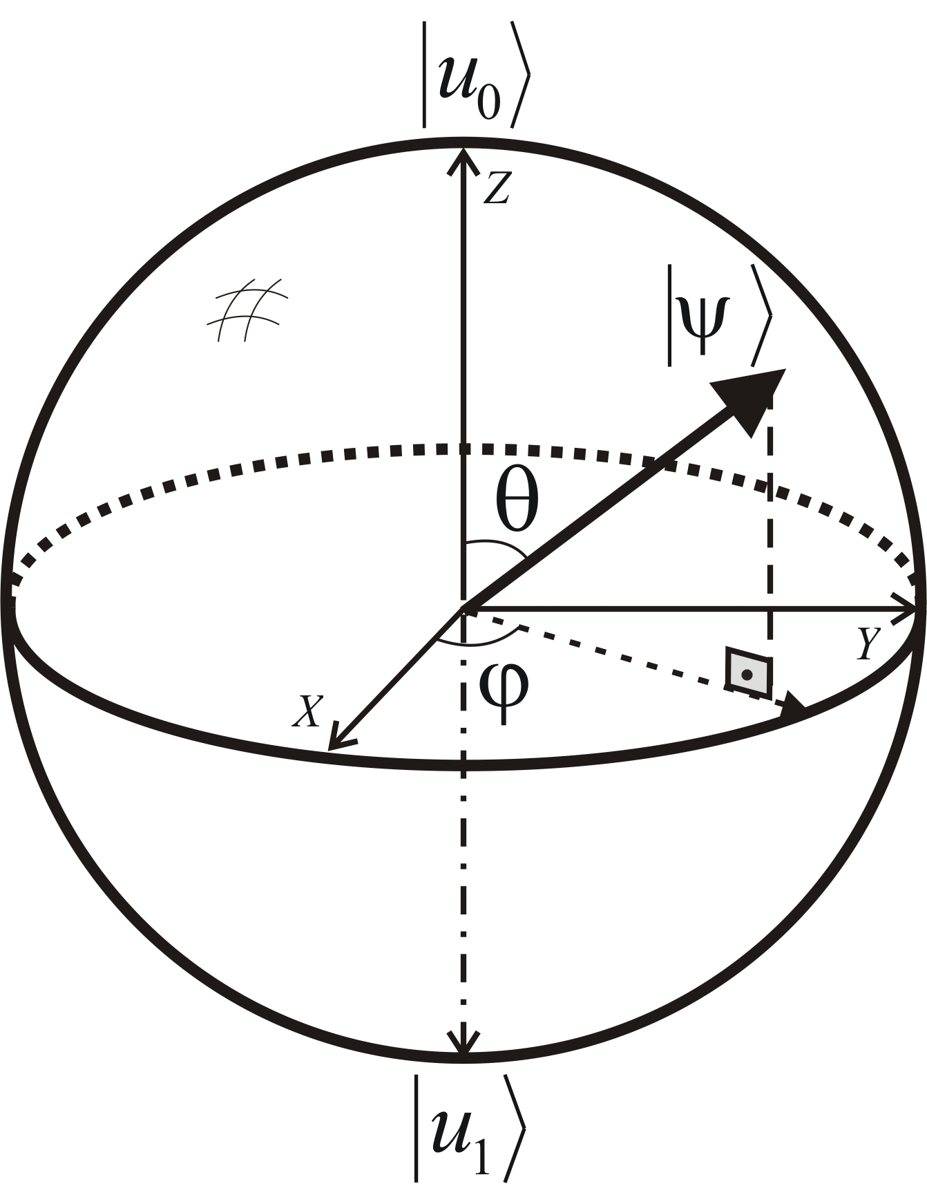
Figure 3: Bloch sphere

The motion is now given instantaneously by a circular motion in turn of an instantaneous axis determined by $P_{0}(t)$ and $P_{1}(t)$ with instantaneous angular velocity

$$\omega(t)=E_{0}(t)-E_{1}(t),$$ (18)

We may introduce coordinates $\theta\prime(t)$ and $\varphi\prime(t)$ for the point $P_{0}(t)$ by the stereographic map

$$\tan\left(\theta\prime/2\right)e^{i\varphi\prime}=(\left\langle u^{0}\right|E_{0}(t)\rangle)^{-1}\left\langle u^{1}\right|E_{0}(t)\rangle.$$ (19)

The right side of the above equation can be computed by the eigenvalue equation:

$${\displaystyle\sum\limits_{\sigma}}\left\langle E^{\tau}\right|\mu_{\sigma}\rangle(H_{\nu}^{\sigma}-E^{\tau}\delta_{\nu}^{\sigma})=0,$$ (20)

giving us

$$\left\{\begin{array}[c]{c}E^{0}=\frac{1}{2}\left[H_{0}^{0}+H_{1}^{1}+\left(\Omega^{2}+4R^{2}\right)^{1/2}\right]\\ E^{1}=\frac{1}{2}\left[H_{0}^{0}+H_{1}^{1}-\left(\Omega^{2}+4R^{2}\right)^{1/2}\right]\end{array}\right.$$ (21)

We make now the following identifications

$$\left\{\begin{array}[c]{l}\lambda(t)=\varphi\prime(t)\\ R(t)=\dfrac{1}{2}\omega(t)\sin\theta\prime(t)\\ \Omega(t)=\omega(t)\cos\theta\prime(t)\end{array}\right.$$ (22)

and we arrive at a very convenient form for our coupled ODE’s over the sphere $\mathbb{CP}(1)$:

$$\left\{\begin{array}[c]{l}\dot{\theta}=\omega(t)\sin\theta\prime(t)\sin(\varphi-\varphi\prime(t))\\ \dot{\varphi}=\omega(t)\left[-\cos\theta\prime(t)+\sin\theta\prime(t)\cot\theta\cos(\varphi-\varphi\prime(t))\right].\end{array}\right.$$ (23)

The three time dependent parameters that describe our hamiltonian can now be directly related to the geometry of the Riemann sphere: $\omega(t)$ gives us the instantaneous angular velocity of the motion in turn of the instantaneous axis of revolution whose direction is described by $(\theta\prime(t),\varphi\prime(t))$. Surprisingly, this seemingly abstract formulation is actually implemented by nature as the motion of an electron spin immersed in a time dependent classical magnetic field given by (see Sakurai (1994), for instance)

$$\vec{B}(t)=\frac{m}{e}\omega(t)\left[\sin\theta\prime(t)\left(\cos\varphi\prime(t)\hat{\imath}+\sin\varphi\prime(t)\hat{\jmath}\right)+\cos\theta\prime(t)\hat{k}\right]\qquad\text{(with }\hslash=c=1\text{)}$$

Let us consider now a very specific kind of motion where the hamiltonian (the point $P_{0}(t)$) describes a uniform rotation on a great circle of the sphere which we choose to be the equator without any loss of generality:

$$\theta\prime(t)=\pi/2\qquad\varphi\prime(t)=\Omega t\qquad\text{and\qquad}\omega=\omega_{0}=\text{constant}$$

Equation (23) becomes then

$$\left\{\begin{array}[c]{l}\dot{\theta}=\omega_{0}\sin(\varphi-\Omega t)\\ \dot{\varphi}=\omega_{0}\cot\theta\cos(\varphi-\Omega t)\end{array}\right.$$ (24)

We choose initial conditions

$$\theta(0)=0\qquad\text{and\qquad}\varphi(0)=0$$ (25)

to match the initial state vector as an energy eigenket. The above initial conditions together with (Eq. 24) lead to

$$\dot{\theta}(0)=0\qquad\text{and\qquad}\dot{\varphi}(0)=0$$ (26)

To prove the adiabatic theorem for this special case, all we need is to assure that for a sufficiently small value of $\Omega/\omega_{0}$ the conditions

$$\theta(t)\approx\pi/2\qquad\text{and\qquad}\varphi(t)\approx\Omega t$$

must hold in a self-consistent manner. Indeed, given that $\varphi\approx\Omega t$, equation (24) implies that $\theta\approx\operatorname{arccot}\left(\Omega/\omega_{0}\right)\approx\operatorname{arccot}\left(0\right)=\pi/2$. To prove the contrary implication, assume $\theta\approx\pi/2$. It is convenient then to introduce new coordinates

$$\left\{\begin{array}[c]{l}\varepsilon(t)=\theta(t)-\pi/2\\ \eta(t)=2(\varphi-\Omega t)\end{array}\right.$$ (27)

which gives us

$$\left\{\begin{array}[c]{l}\dot{\varepsilon}=\omega_{0}\sin\left(\eta/2\right)\\ \dot{\eta}=-2\left[\Omega+\omega_{0}\tan\varepsilon\cos\left(\eta/2\right)\right]\end{array}\right.\qquad\text{with\qquad}\left\{\begin{array}[c]{l}\varepsilon(0)=0\\ \eta(0)=0\end{array}\right.\qquad\text{and}\qquad\left\{\begin{array}[c]{l}\dot{\varepsilon}(0)=0\\ \dot{\eta}(0)=-2\Omega\end{array}\right.$$ (28)

By taking the time derivative of the second equation (28) and using the first equation together with the condition $\theta(t)\approx\pi/2\Longrightarrow\varepsilon\approx 0$ one gets the approximate differential equation

$$\ddot{\eta}\approx-\omega_{0}^{2}\sin\eta$$ (29)

which we recognize immediately as the well-known simple pendulum equation (from undergraduate classical mechanics) with “conserved energy” given by

$$E=T+U=\frac{1}{2}\dot{\eta}^{2}-\omega_{0}^{2}\cos\eta$$ (30)

It follows from the initial conditions in (28) that the “total mechanical energy” of the pendulum is

$$E=2\Omega^{2}-\omega_{0}^{2}$$ (31)

with minimum “potential energy” at $U(\eta_{\min})=U(0)=-\omega_{0}^{2}$. It is easy to see in this set up that one can confine the motion as close as one desires to $\eta_{\min}=0$ by making the ratio $\omega_{0}/\Omega$ as larger as necessary. So we have that the implication $\theta\approx\pi/2\Longrightarrow\varphi\approx\Omega t$ must hold true.

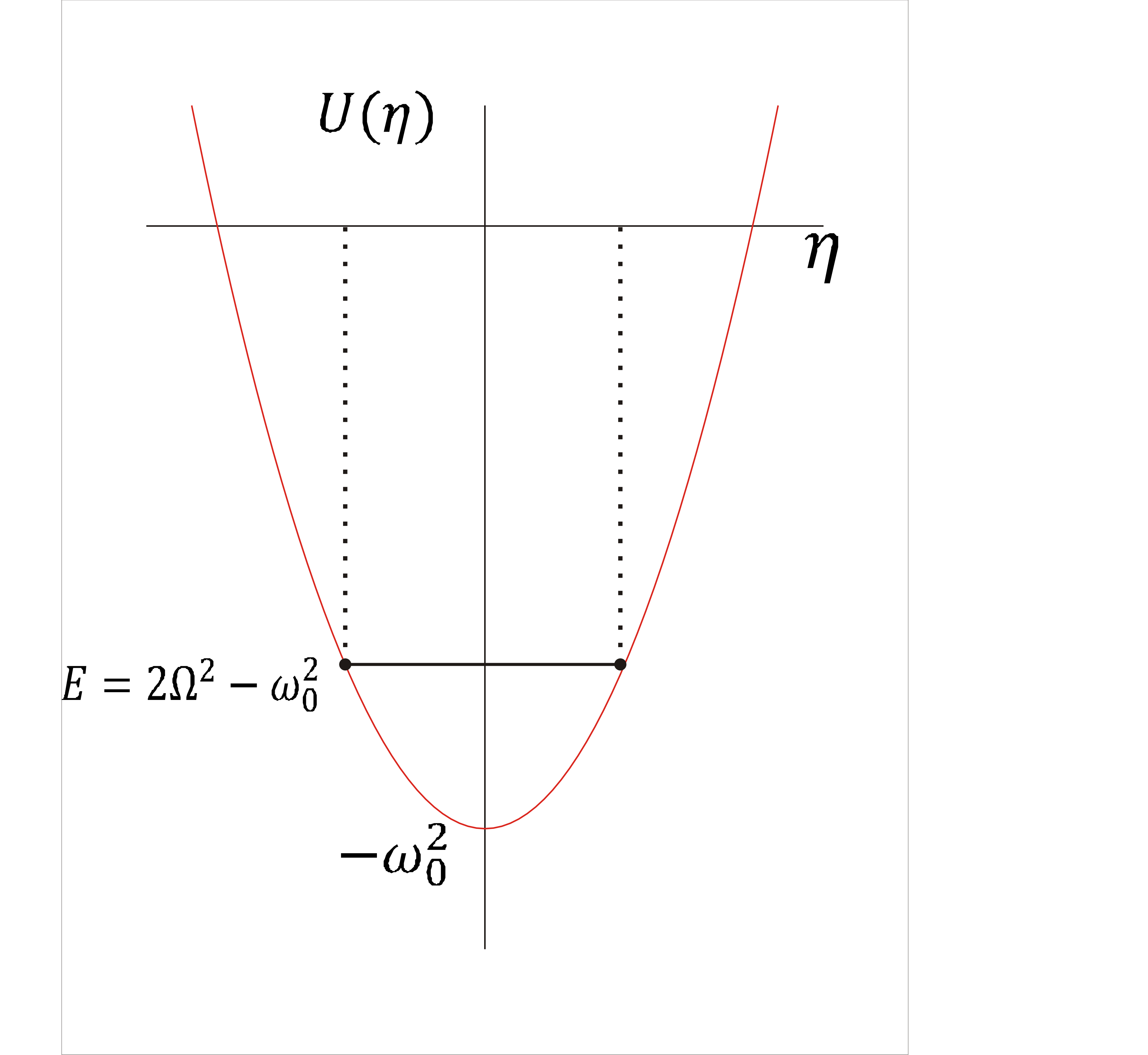
Figure 4: Potential energy.

To extend the proof to an arbitrary path over the sphere one must only need to remember that such path can be divided in $N$ (let us say equal segments) sub-paths with $N$ sufficiently large so that each segment may be considered as approximately a geodesic path in such a way that the above argument can be applied piece-wise.

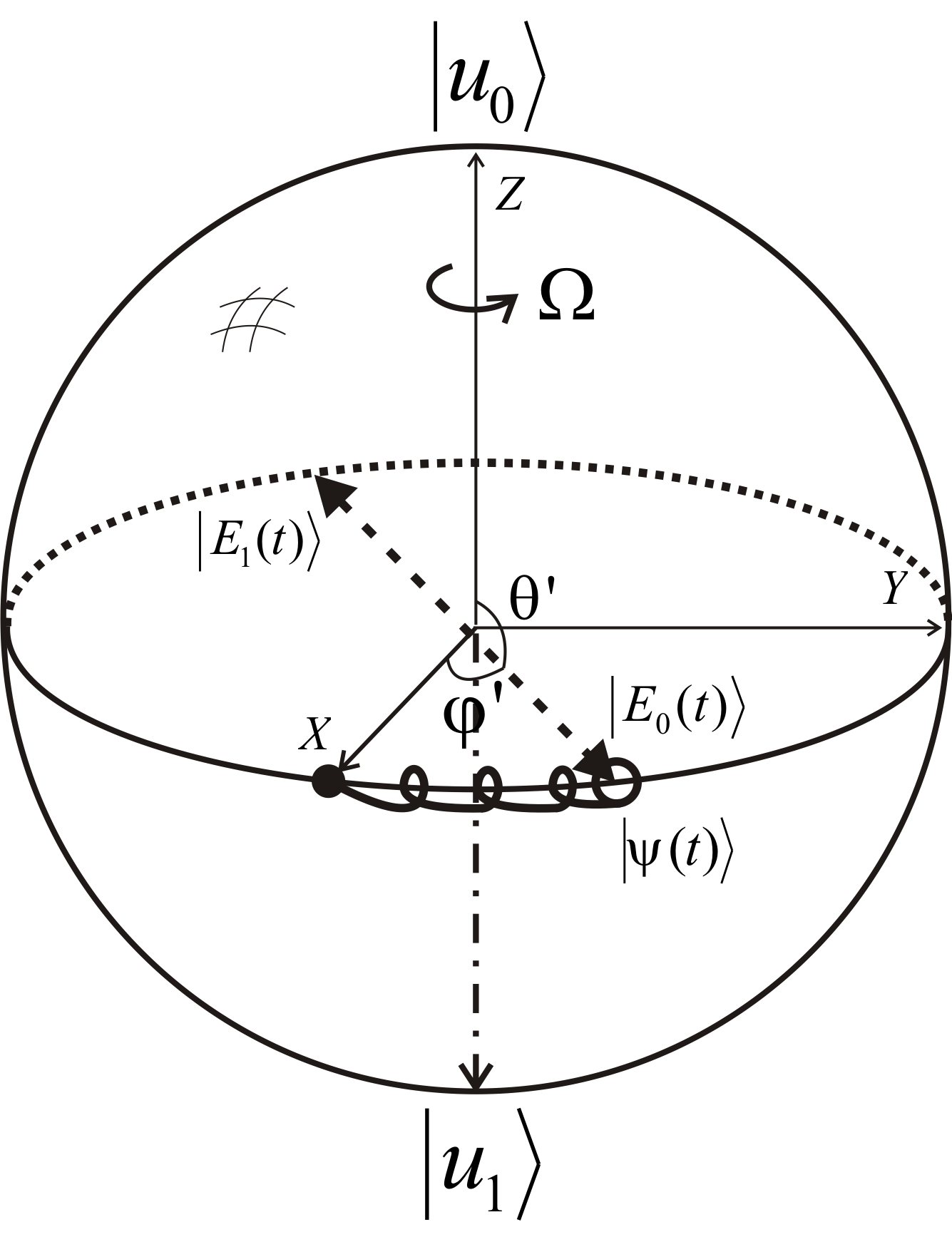
Figure 5: A pictorial representation of our simplified model of the adiabatic theorem in action.

We have plotted below some numerical implementations of our simplified model (Eq. 24) with different values of $\omega_{0}/\Omega$:

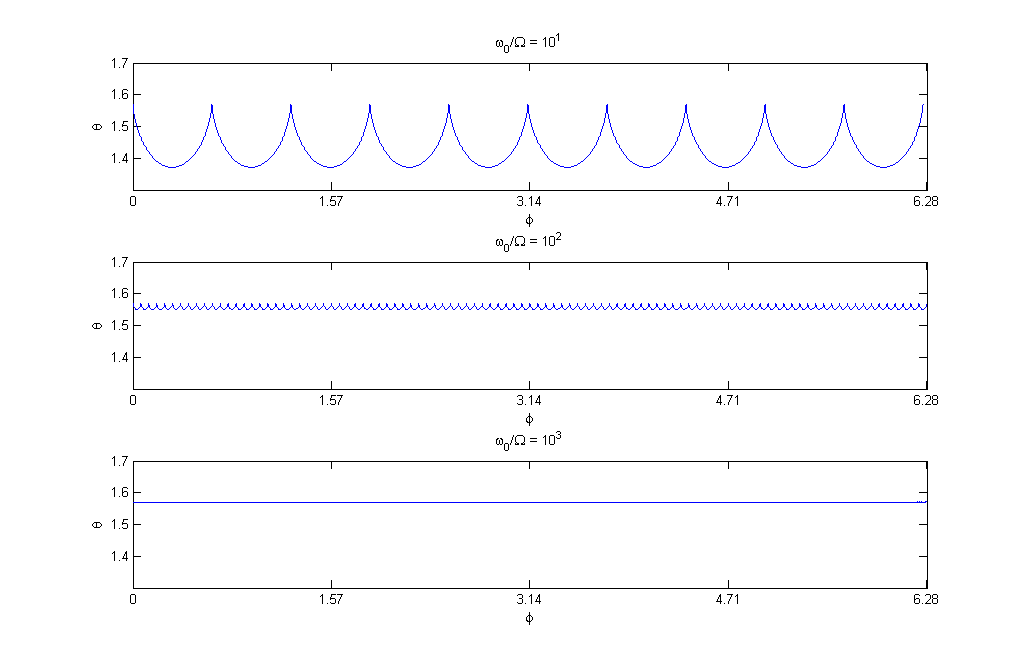
Figure 6: Three plots for $\omega_{0}/\Omega$ respectively given by $10^{1},10^{2}$ and $10^{3}$.

The above analysis shows convincingly that the projected state “whirls” in turn of the instantaneous north pole evermore tightly as the factor $\omega_{0}/\Omega$ gets larger and larger.

III Concluding remarks

We have briefly reviewed the geometry of quantum mechanics developed back in the eighties by Aharonov  and Anandan among others. We used these ideas to present an elementary geometric argumentation for the validity of the adiabatic theorem. We have used only the minimum geometric structure needed for an understanding of the adiabatic theorem, but there are many rich structures in the geometry of quantum mechanics. We refer the reader to Arnold (1989); Kibble (1979); Page (1987); Brody and Hughston (2001) for more details on these matters.

Though we do not claim this as a complete proof, we are sure that this geometric reasoning can be easily implemented as a rigorous proof for those analytically inclined. We hope that this geometric picture is sufficiently straightforward to turn the concept of quantum adiabatic computation into a much more understandable tool for undergraduate students of physics and even for specialists.

The modern theories of quantum computation and information have become a central research field in physics and the quest for the best models of quantum computing (quantum gate model, adiabatic quantum computing, cluster or measurement-based quantum computation) and even to establish the equivalence (or not) between their true powers of computation (computability and complexity classes) are still open questions. A better intuitive understanding and presentation of the key physical and mathematical structures behind their functioning seems to be a sensible enterprise. We believe to have presented the most direct and pedagogical frame so far of this important theorem, at least for two level systems.

References

- Born and Fock [1928] M. Born and V. Fock, Zeitschrift für Physik A Hadrons and Nuclei 51, 165 (1928), ISSN 0939-7922, 10.1007/BF01343193.
- Kato [1950] T. Kato, J. Phys. Soc. Japan 5, 9 (1950).
- Berry [1984] M. Berry, Proceedings of the Royal Society of London. Series A, Mathematical and Physical Sciences 392, 45 (1984), ISSN 0080-4630.
- Aharonov and Anandan [1987] Y. Aharonov and J. Anandan, Physical Review Letters 58, 1593 (1987), ISSN 1079-7114.
- Farhi et al. [2000] E. Farhi, J. Goldstone, S. Gutmann, and M. Sipser, Arxiv preprint quant-ph/0001106 (2000).
- Aharonov et al. [2004] D. Aharonov, W. Van Dam, J. Kempe, Z. Landau, S. Lloyd, and O. Regev, in Foundations of Computer Science, 2004. Proceedings. 45th Annual IEEE Symposium on (IEEE, 2004), pp. 42–51.
- Marzlin and Sanders [2004] K. Marzlin and B. Sanders, Physical review letters 93, 160408 (2004).
- Wu and Yang [2005] Z. Wu and H. Yang, Physical Review A 72, 012114 (2005).
- Tong et al. [2005] D. M. Tong, K. Singh, L. C. Kwek, and C. H. Oh, Phys. Rev. Lett. 95, 110407 (2005).
- Ma et al. [2006] J. Ma, Y. Zhang, E. Wang, and B. Wu, Physical review letters 97, 128902 (2006).
- Wei and Ying [2007] Z. Wei and M. Ying, Physical Review A 76, 024304 (2007).
- Amin [2009] M. Amin, Physical review letters 102, 220401 (2009).
- Boixo and Somma [2010] S. Boixo and R. Somma, Physical Review A 81, 032308 (2010).
- Frasca [2011] M. Frasca, Arxiv preprint arXiv:1107.4971 (2011).
- Rigolin and Ortiz [2011] G. Rigolin and G. Ortiz, Arxiv preprint arXiv:1111.5333 (2011).
- Griffiths [2005] D. Griffiths, Introduction to quantum mechanics, vol. 1 (Pearson Prentice Hall, 2005).
- Messiah [1999] A. Messiah, Quantum Mechanics, vol. 1-2 (Dover Publications, 1999).
- Kasuga [1961] T. Kasuga, Proceedings of the Japan Academy, Series A, Mathematical Sciences 37, 366 (1961).
- Anandan and Aharonov [1990] J. Anandan and Y. Aharonov, Phys. Rev. Lett. 65, 1697 (1990).
- Brody [2003] D. Brody, Journal of Physics A: Mathematical and General 36, 5587 (2003).
- Sakurai [1994] J. J. Sakurai, Modern Quantum Mechanics (Addison Wesley, 1994), 2nd ed., ISBN 0201539292.
- Arnold [1989] V. Arnold, Mathematical methods of classical mechanics, vol. 60 (Springer, 1989).
- Kibble [1979] T. Kibble, Communications in Mathematical Physics 65, 189 (1979).
- Page [1987] D. Page, Physical Review A 36, 3479 (1987), ISSN 1094-1622.
- Brody and Hughston [2001] D. Brody and L. Hughston, Journal of Geometry and Physics 38, 19 (2001).