The Role of Power-Law Correlated Disorder in the Anderson Metal-Insulator Transition

Abstract

We study the influence of scale-free correlated disorder on the metal-insulator transition in the Anderson model of localization. We use standard transfer matrix calculations and perform finite-size scaling of the largest inverse Lyapunov exponent to obtain the localization length for respective 3D tight-binding systems. The density of states is obtained from the full spectrum of eigenenergies of the Anderson Hamiltonian. We discuss the phase diagram of the metal-insulator transition and the influence of the correlated disorder on the critical exponents.

1 Introduction

The possibility of having phase transitions in disordered systems, which contain randomness as a central ingredient, has attracted a lot of interest over past decades. Prototypical examples of classical and quantum disordered systems are the percolation problem BroH57 and the Anderson model of localization And58 , respectively. Over the years, the respective transitions – percolation and Anderson metal-insulator transition (MIT) – have been intensively studied Ess80 ; StaA92 ; Isi92 ; LeeR85 ; KraM93 . Typically, the random numbers, which represent the disorder, are taken to be uncorrelated. However, in realistic systems, where, for example, the disorder is induced by a complex environment surrounding the system sites, one expects to find correlations between the random numbers. Spatial correlations can be characterized according to their behavior on different length scales. For example, they might become irrelevant if the length scales associated with the phase transition are larger than a characteristic correlation length. On the other hand, there is also scale-free disorder, which is found in many physical systems Isi92 ; PenBGH92 ; VidMNM96 . Here, the correlations are taking effect on all length scales. These long-range correlations are characterized by a power-law behavior, $C(\bf{r}-\bf{r^{\prime}})\propto|\bf{r}-\bf{r^{\prime}}|^{-\alpha}$. Here, $C(\bf{r}-\bf{r^{\prime}})$ denotes the correlation function and $\alpha$ is the correlation exponent.

For the (classical) percolation problem it was found that the presence of scale-free disorder has a profound influence on the percolation transition. For this situation, the extended Harris criterion Har74 ; Har83 ; WeiH83 ; Wei84 predicts a crossover of the critical exponent $\nu$ from its value $\nu_{0}$ for uncorrelated random numbers to $2/\alpha$ provided the decay of the correlations is sufficiently weak, $\alpha<2/\nu_{0}$.

In the present paper we address the question of the role of power-law correlations for the Anderson transition in disordered electronic systems. Originally, in his seminal paper Anderson showed that extended electronic states can become spatially localized due to the presence of uncorrelated disorder And58 . As a consequence, the system undergoes a phase transition from a conducting phase (for extended states) to an insulating phase (for localized states), which can be characterized by a critical exponent. In a previous study NdaRS04 it was found, that the critical exponent is independent of the correlation exponent for a transition at fixed energy in the center of the band, while for a transition at fixed disorder strength the critical exponent obeys the extended Harris criterion. However, the calculations have been performed using a modified transfer-matrix method (TMM), which consists of forward and backward TMM calculations for a quasi-one-dimensional (quasi-1D) block of length $L_{0}\sim 10^{3}$. This artificial periodicity might have an additional influence on the transition. To avoid this issue, we use the standard TMM KraM93 for calculating the localization length of quasi-1D systems with a length $L=4\cdot 10^{5}$. Subsequently performing a finite-size scaling (FSS) analysis provides us with estimates of the critical points SleO99a for different correlation exponents. The critical points are summarized in a phase diagram showing the influence of the correlations on the phase boundary. This is the central result of the present paper. Additionally, we calculate the density of states (DOS) of 3D systems in the presence of scale-free disorder.

The paper is organized as follows. In the next section, we introduce the Anderson model of localization and briefly summarize the main properties of the associated phase transition. Moreover, we provide an overview of the numerical methods we use to calculate the properties of the transition. In Sec. 3 we present our results for transitions at fixed energy and fixed disorder. Then the phase-diagram of the Anderson MIT in the presence of scale-free disorder is discussed and the relation to the DOS is investigated. Finally, in the last section we summarize and discuss our results.

2 Model and Numerical Methods

2.1 Anderson Model of Localization with Long-Range Correlated Disorder

The Anderson model And58 ; KraM93 is widely used to investigate the phenomenon of localization in disordered materials. It is based upon a tight-binding Hamiltonian in site representation

$$\mathcal{H}=\sum_{\bf i}\varepsilon_{\bf i}|{\bf i}\rangle\langle{\bf i}|-\sum_{\bf i\,j}\,t_{{\bf ij}}\,|{\bf i}\rangle\langle{\bf j}|\;,$$ (1)

where $|{\bf i}\rangle$ is a localized state at lattice site ${\bf i}$. The matrix elements $t_{{\bf ij}}$ denote hopping integrals between states at sites ${\bf i}$ and ${\bf j}$. Typically, hopping is restricted to nearest neighbors. The on-site potentials $\varepsilon_{\bf i}$ are random numbers, chosen according to some probability distribution $P(\varepsilon)$ characterized by the mean $\langle\varepsilon_{i}\rangle$ and the correlation function $C(|\mbox{\boldmath$\ell$}|)\propto\sum_{{\bf i}}\langle\varepsilon_{\bf i}\varepsilon_{{\bf i}+\mbox{\boldmath$\ell$}}\rangle$. However, usually the site energies are taken to be statistically independent. For example, convenient choices of $P(\varepsilon)$ are a box distribution of width $W$ or a Gaussian white noise distribution, both with $\langle\varepsilon_{\bf i}\rangle=0$ and $C(|\mbox{\boldmath$\ell$}|)=\frac{W^{2}}{12}\delta_{|\mbox{\boldmath$\ell$}|,0}$. Other distributions have also been considered KraM93 ; OhtSK99 ; RomS03 .

For uncorrelated potentials the resulting situation may be summarized as follows KraM93 : for strong enough disorder, $W>W_{\rm c}(0)$, all states are exponentially localized to a region of finite size. The extent of this region is characterized by the so-called localization length $\lambda$. The value of the critical disorder strength $W_{\rm c}$ depends on the distribution $P(\varepsilon)$ and the dimension $d$ of the system. The value of $W_{\rm c}$ additionally depends on the Fermi energy $E$ and the curve $W_{\rm c}(E)$ separates localized states, $W>W_{\rm c}(E)$, from extended states, $W<W_{\rm c}(E)$, in the phase diagram. If instead of $E$ the disorder strength is fixed, there will be a critical energy $E_{\rm c}(W)$ and states with $|E|<E_{\rm c}$ are extended and those with $|E|>E_{\rm c}$ localized. The transition from extended to localized wave-functions at the critical point is called disorder driven or Anderson MIT. In the vicinity of the critical point the localization length behaves as

$$\lambda(\tau)\propto\left|\tau_{\rm c}-\tau\right|^{-\nu}\;,$$ (2)

where $\tau$ is either $E$ or $W$. The critical exponent $\nu$ characterizes the phase transition and is expected to be universal.

In the present work we are interested in the influence of long-range correlated disorder potentials on the Anderson MIT. In particular, we study the dependence of the critical points and the critical exponents on the strength of the correlations. To this end we use random potentials generated from a Gaussian probability distribution and with a correlation function of the form

$$C(\mbox{\boldmath$\ell$})\equiv\langle\varepsilon_{\bf i}\varepsilon_{{\bf i}+\mbox{\boldmath$\ell$}}\rangle\propto|\mbox{\boldmath$\ell$}|^{-\alpha}\;,$$ (3)

where $\alpha$ is the correlation exponent which determines the strength of the correlations. In contrast to short-range correlations the power-law behavior in Eq. (3) does not introduce a characteristic length scale and therefore the disorder is said to be scale-free.

In general, it is extremely complicated to obtain analytical results of transport properties for the Anderson model of localization. For example, only in the case of $d=1$ rigorous proofs of strong localization for all energies and disorder strengths have been given GolMP77 . Moreover, the explicit energy and disorder strength dependence of the localization length for weak disorder has been derived Tho79 ; PasF92 . There are also some results for 1D systems with long-range correlated disorder. For energies close to the band center a weak disorder expansion for $\lambda$ has been derived in Ref. IzrK99 , which shows the dependence of the localization length on the correlations via a Fourier transform of the correlation function. Here, the localization length is proportional to $W^{-2}$. On the other hand at the unperturbed band edge ($|E|=2$) it was found DerG84 ; RusHW98 that $\lambda(E=2,W)\propto W^{-y}$ with $y=2/3$ for $\alpha=\infty$ and $y=2/(4-\alpha)$ for $\alpha\leq 1$.

2.2 Numerical Methods

In order to investigate the influence of scale-free correlations on the Anderson MIT, we first generate the correlated on-site potential for systems of size $M\times M\times L$ using a modified Fourier filtering method (FFM) MakHSS96 with one additional step. Namely, after performing the usual FFM we shift and scale the obtained sequence of correlated random numbers such that the mean vanishes and the variance is $W^{2}/12$.

As mentioned in the introduction, the localization length $\lambda$ is calculated using a standard TMM KraM93 . Thereby we use a new seed for each parameter combination ($E$, $W$, $\alpha$, $M$). Lastly, the critical exponent, mobility edge and critical disorder are obtained from the FSS analysis SleO99a based on a higher-order expansion of Eq. (2) at the transition ($\tau=\tau_{\rm c}$). This procedure is outlined in appendix A. The error resulting from the associated fitting procedure should not be seen as an upper (or lower) bound for the critical parameters, but rather as a qualitative measure for the stability of the fitting procedure. A reliable estimate of the numerical uncertainty requires a more sophisticated error analysis MilRS00 .

Another issue connected with the FSS method are the corrections to scaling. Generally, for small systems one would always expect to find finite-size corrections and consequently one should include corrections to scaling in the analysis. However, this also increases the number of parameters to be fitted tremendously and makes it sometimes complicated to find a reasonable fit. One possibility to partly circumvent this problem is ignoring the small system sizes (in our analysis below this means $M=5,7$) and doing the FSS without corrections.

The DOS is obtained from the full spectrum of eigenenergies of the 3D Anderson Hamiltonian for systems of size $M^{3}$. The eigenenergies are calculated using standard matrix diagonalization methods lapack . Since the accessible maximum system size is restricted by the numerical resources, the results are averaged over a large number of disorder realizations to decrease statistical fluctuations. Furthermore the symmetry of the DOS with respect to $E=0$ is utilized.

3 Numerical Results and Discussion

3.1 Numerical Calculations

In order to study the localization length in the presence of correlated disorder we focus on quasi-1D systems with $L=400000$ and $M=5,7,9,11,13$ and $15$. The error of the localization length is determined from the variance of the change of the Lyapunov exponent during the TMM iterations MacK81 ; MacK83 . The accuracy of the localization length is therefore limited by the finite length of the considered systems. To give an impression of the quality of the TMM results and the FSS fitting procedure Fig. 1 shows the reduced localization length $\Lambda=\lambda/M$ versus disorder strength $W$ for $E=6.0$ and $\alpha=2.5$. In Fig. 1a the raw data for $\Lambda$ obtained from the TMM calculation are shown for various system sizes. Performing the FSS procedure taking corrections to scaling into account one obtains the curves shown in Fig. 1a. Considering no corrections to scaling we obtain the fits shown in Fig. 1b. In this case, ignoring the small systems leads to almost the same critical values. In the following we will concentrate on results obtained without taking corrections to scaling into account.

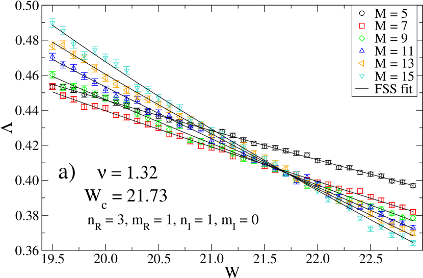
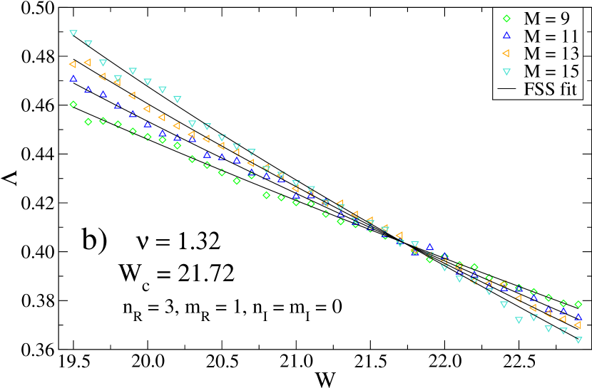
Figure 1: Reduced localization length $\Lambda$ vs disorder strength $W$ for $E=6.0$ and $\alpha=1.5$. Solid lines show the FSS fit to numerical data (a) for all system sizes $M$ taking corrections to scaling into account and (b) for $M>7$ without corrections to scaling. The resulting critical exponent $\nu$ and disorder strength $W_{\rm c}$ are shown together with the respective expansion orders of the FSS (cf. appendix A).

The DOS is computed for disorder strengths $W=1.5,$ $\ldots,$ $30$ for the uncorrelated and a long-ranged correlated potential ($\alpha=0.9$), respectively. The size of the systems is $M^{3}=22^{3}$. Results are averaged over at least $1000$ disordered samples. For the ordered system, $W=0$, the DOS is calculated by the diagonalization of a single system with $M^{3}=30^{3}$.

3.2 Transition at Fixed Energy

First we focus on the Anderson MIT for fixed energy ($E=\rm{const.}$). The values of the respective critical parameters are shown in Tab. 1. One sees that for uncorrelated disorder ($\alpha=\infty$) the obtained critical exponents, $\nu$, are consistent with the high-precision value $\nu_{0}=1.58\pm 0.03$ of Ref. SleO99a . For $E=0$ the critical disorder strength agrees very well with the value found previously SleO99a , $W_{\rm c}=21.29\pm 0.01$.

In the presence of long-range correlations the critical exponent remains close to the value for uncorrelated disorder potentials at least for energies well inside the band of the system without disorder. For energies close to the band edge ($|E|=6$) of such systems the critical exponent is smaller than $\nu_{0}$ in case of a long-range correlated potential. However, at the same time the estimated error of the exponents becomes larger and is more sensitive to changing the fitting parameters. The error for the critical disorder is relatively small independently of the value of $\alpha$ and one finds that the value is more stable than $\nu$ against changing the fitting parameters.

The value of $W_{\rm{c}}$ is monotonically increasing for decreasing $\alpha$. In other words the MIT sets in for a larger disorder strength compared to the uncorrelated case. This supports the intuitive expectation of an effective smoothening of the random potential due to the correlations. For 1D systems and weak disorder it has been shown that the effective disorder is given in terms of the Fourier transform of the correlation function IzrK99 . In the center of the band this leads to an increasing localization length for smaller correlation exponents CroCS11 .

	$\alpha$	$E$	$W_{\rm c}$	$\triangle W_{\rm c}$	$\nu$	$\triangle\nu$
	$\infty$	$0.0$	$21.28$	$0.04$	$1.56$	$0.08$
	$\infty$	$2.0$	$20.600$	$0.024$	$1.54$	$0.05$
	$\infty$	$4.0$	$18.276$	$0.029$	$1.56$	$0.06$
	$\infty$	$5.43$	$14.81$	$0.04$	$1.55$	$0.08$
	$2.5$	$0.0$	$23.50$	$0.04$	$1.55$	$0.08$
	$2.5$	$2.0$	$22.92$	$0.07$	$1.57$	$0.18$
$\dagger\;$	$2.5$	$4.0$	$21.25$	$0.07$	$1.57$	$0.11$
$\ddagger\;$	$2.5$	$5.43$	$19.04$	$0.05$	$1.43$	$0.09$
	$1.5$	$0.0$	$25.76$	$0.05$	$1.69$	$0.22$
	$1.5$	$2.0$	$25.37$	$0.03$	$1.60$	$0.06$
	$1.5$	$4.0$	$24.22$	$0.05$	$1.54$	$0.09$
	$1.5$	$5.43$	$22.63$	$0.07$	$1.45$	$0.11$
	$1.5$	$6.0$	$21.72$	$0.04$	$1.32$	$0.05$
	$0.9$	$0.0$	$29.25$	$0.08$	$1.64$	$0.27$
	$0.9$	$2.0$	$28.99$	$0.08$	$1.61$	$0.14$
	$0.9$	$4.0$	$28.11$	$0.08$	$1.45$	$0.11$
	$0.9$	$5.43$	$26.82$	$0.07$	$1.38$	$0.08$
	$0.9$	$7.0$	$24.72$	$0.13$	$1.23$	$0.12$

Table 1: Critical disorder $W_{\rm c}$ and exponent $\nu$ obtained from FSS analysis without taking corrections to scaling into account. The errors indicate the confidence interval of the fit. The symbols $\dagger$ and $\ddagger$ denote parameters coinciding in Tables 1 and 2.

3.3 Transition at Fixed Disorder Strength

	$\alpha$	$W$	$E_{\rm c}$	$\triangle E_{\rm c}$	$\nu$	$\triangle\nu$
	$\infty$	$6.0$	$6.52$	$0.03$	$1.49$	$0.20$
	$\infty$	$12.0$	$6.173$	$0.009$	$1.64$	$0.03$
	$\infty$	$16.5$	$4.855$	$0.017$	$1.58$	$0.05$
	$\infty$	$19.0$	$3.545$	$0.019$	$1.59$	$0.04$
	$2.5$	$6.0$	$6.615$	$0.015$	$1.58$	$0.06$
	$2.5$	$12.0$	$6.826$	$0.010$	$1.801$	$0.028$
	$2.5$	$16.5$	$6.232$	$0.011$	$1.883$	$0.029$
$\ddagger\;$	$2.5$	$19.0$	$5.428$	$0.013$	$1.92$	$0.03$
$\dagger\;$	$2.5$	$21.38$	$4.02$	$0.03$	$1.96$	$0.05$
	$1.5$	$6.0$	$6.718$	$0.028$	$1.57$	$0.09$
	$1.5$	$12.0$	$7.484$	$0.017$	$1.93$	$0.04$
	$1.5$	$16.5$	$7.329$	$0.023$	$2.03$	$0.07$
	$1.5$	$19.0$	$7.056$	$0.027$	$2.30$	$0.11$
	$0.9$	$6.0$	$6.52$	$0.04$	$1.64$	$0.27$
	$0.9$	$12.0$	$7.35$	$0.03$	$1.93$	$0.08$
	$0.9$	$16.5$	$7.71$	$0.05$	$2.03$	$0.20$
	$0.9$	$19.0$	$7.70$	$0.04$	$2.19$	$0.06$

Table 2: Critical energy $E_{\rm c}$ and exponent $\nu$ obtained from FSS analysis without taking corrections to scaling into account. The errors indicate the confidence interval of the fit.

$\alpha$	$W$	$E_{\rm c}$	$\triangle E_{\rm c}$	$\nu$	$\triangle\nu$	$y$	$\triangle y$
$1.5$	$12.0$	$7.79$	$0.07$	$1.93$	$0.05$	$2.37$	$0.24$
$1.5$	$16.5$	$7.56$	$0.05$	$2.16$	$0.05$	$3.5$	$0.4$
$1.5$	$19.0$	$7.13$	$0.05$	$2.26$	$0.09$	$4.5$	$0.8$

Table 3: Critical energy $E_{\rm c}$ and exponent $\nu$ from FSS analysis with taking corrections to scaling into account. The errors indicate the confidence interval of the fit.

Next, we consider the case of transitions at fixed disorder strength ($W={\rm const.}$). The respective results for critical energies and exponents are summarized in Tab. 2. For comparison Tab. 3 contains some FSS results obtained with corrections to scaling taken into account.

For uncorrelated random potentials previous studies showed that the critical exponent of the transition at fixed disorder is, within error bars, identical to the exponent obtained for the transition at fixed energy. Here, we also find a good agreement with the respective exponent shown in Tab. 1 and with the high-precision value $\nu_{0}$ SleO99a . Further, the critical disorder strengths are in accordance with the results of Ref. BulSK87 .

In contrast to the transition at fixed energy discussed earlier, in the presence of long-range correlations the critical exponents are larger than the respective exponent obtained for uncorrelated potentials for all disorder strengths except $W=6.0$. Moreover, the mobility edge is systematically shifted towards higher energies.

3.4 Phase Diagram and DOS

Combining Tabs. 1 and 2 we obtain a complete phase diagram of the Anderson model in presence of long-range correlated disorder, which is shown in Fig. 2. The phase diagram reflects the general features we have discussed for the two transitions. In the presence of long-range correlations the metallic phase space grows, pushing the mobility edge to larger disorder strengths and higher energies.

Figure 3 illustrates the influence of long-range correlated disorder on the DOS. The contours in Fig. 3 show the characteristic broadening of the DOS for increasing disorder strength $W$ BulSK87 . The difference between correlated and uncorrelated disorder is much less pronounced than in the phase diagram. Around the band center ($E<2$) the DOS is increased by correlations. Toward the band edges the DOS is slightly smaller. From Figs. 2 and 3 we can conclude that the mobility edge is always clearly inside the band and comes close to the band edge only for small disorder strengths $W$.

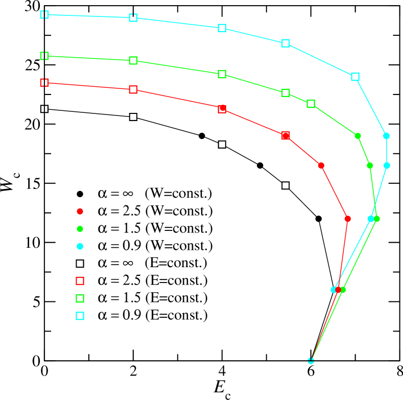
Figure 2: Phase diagram of the Anderson model with long-range correlated disorder. Open and filled symbols indicate transitions at fixed energy and fixed disorder strength, respectively. Lines are a guide to the eye only.

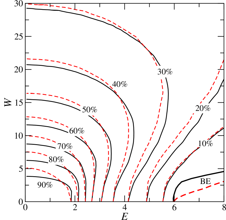
Figure 3: The contour diagram shows the disorder dependence of the DOS for the uncorrelated (black) and a correlated potential with $\alpha=0.9$ (red dashed). Lines are drawn at the given percentage of the maximum value of the DOS located at $W=0$ and $E=0$. The band edge (BE) is estimated by the largest eigenenergy observed.

One might also ask how the two transitions behave at the same point in the phase diagram. A previous study of the Anderson model with uncorrelated disorder suggested that close to the band edge and for fixed disorder strength the critical exponent may be different from $\nu_{0}$ KraBMS90 . However, strong finite-size effects in this region did not allow a conclusive answer. A more recent study indicates that for both transitions at different points in the phase diagram the same exponent is obtained BrnM06 . From Fig. 2 we see that there are two pairs $(W_{\rm c},E_{\rm c})$ which denote the same phase-diagram point, respectively. The critical parameters for these points are marked in Tabs. 1 and 2 by $\dagger$ and $\ddagger$. In Fig. 2 these points are conspicuous, because the (red) open squares and filled circles coincide. In both cases the transitions at fixed energy yield a critical exponent in agreement with $\nu_{0}$, while the exponents of transitions at fixed disorder strength are larger than $\nu_{0}$. A similar behavior has been reported in Ref. NdaRS04 , where in addition an agreement of the critical exponents of the transition at fixed disorder strength with the extended Harris criterion was found. Due to the limited accuracy of our numerical data and the sensitivity of the critical exponent, we cannot give a quantitative comparison with the Harris criterion. Nevertheless, it is interesting to notice, that in our case the critical exponents strongly depend on the value of $W$ and only weakly on the value of $\alpha$. Moreover, there is a possible connection of the behavior of $\nu$ and the slope of the curve describing the phase boundary, $W_{\rm c}(E)$ and $E_{\rm c}(W)$, respectively. For example, for fixed disorder strength the critical exponents increase with increasing magnitude of $dE_{\rm c}(W)/dW$. In other words, only if the chosen path through the phase diagram is perpendicular to the phase boundary, we obtain an unchanged critical exponent from the FSS analysis compared to the uncorrelated value $\nu_{0}$. Otherwise the estimated exponent is different from $\nu_{0}$. A detailed investigation of this behavior would certainly be very interesting and might help to elucidate the role of long-range correlations for the Anderson MIT.

4 Summary and Conclusions

In summary, we have studied the role of scale-free disorder in the Anderson MIT. The correlations are characterized by a power-law with a correlation exponent. The characteristics of the Anderson transition have been obtained from the numerically calculated behavior of the localization length in quasi-1D systems. We employed a standard TMM computation and estimated the critical exponents and critical points using a FSS analysis for different correlation exponents. Further, we obtained the phase diagram for the Anderson MIT in presence of scale-free disorder.

We observe a shift of the phase boundary towards higher energies and stronger disorder, respectively. The latter may be understood as a result of an effective smoothening of the disorder potential in presence of correlations. A similar behavior has been observed for 1D systems, where the localization length increases for smaller correlation exponents.

Regarding the critical exponents we cannot draw quantitative conclusions due to the high sensitivity of the fitted results. However, qualitatively we see strong indications that the critical exponents behave differently for transitions at fixed energy and fixed disorder strength as it was reported before NdaRS04 . For fixed energies $|E|>6$ the critical exponent remains consistent with the value for uncorrelated disorder, while for fixed disorder strengths $W$ the exponent increases for increasing $W$. Further investigations in this direction would certainly be helpful to get a better understanding of the role of correlations for the Anderson MIT.

Appendix A Finite-Size Scaling

A problem one is always faced with when using numerical methods to investigate phase transitions, is the fact that for finite systems there can be no singularities induced by a transition and the divergences are always rounded off Car96 . However, the phase transition can still be studied using FSS. Specifically, near the MIT one expects the following one-parameter scaling law for the reduced localization length Car96

$$\Lambda(M,\tau,b)=\mathcal{F}\left(\frac{M}{b},\chi(\tau)b^{1/\nu},\phi(\tau)b^{-y}\right)\;,$$ (A.1)

where $b$ is the scale factor, $\chi$ is a relevant scaling variable, $\phi$ is an irrelevant scaling variable, $\nu>0$ is the critical exponent and $y>0$ is the irrelevant scaling exponent. The irrelevant scaling variable allows us to take account of corrections to scaling due to the finite size of the sample. Here, the parameter $\tau$ measures the distance from the mobility edge $E_{\rm c}$, $\tau=|E-E_{\rm c}|/E_{\rm c}$, or the distance from the critical disorder strength $W_{\rm c}$, $\tau=|W-W_{\rm c}|/W_{\rm c}$. The choice $b=M$ leads to the standard scaling form

$$\Lambda(M,\tau)=F(M^{1/\nu}\chi(\tau),M^{-y}\phi(\tau))$$ (A.2)

with $F$ being trivially related to $\mathcal{F}$. For $\tau$ close to zero we expand $F$ into a Taylor series up to order $n_{\rm I}$ and obtain a series of functions $F_{n}$ SleO99a

$$\Lambda(M,\tau)=\sum\limits^{n_{\rm I}}_{n=0}\phi^{n}M^{-ny}F_{n}(\chi M^{1/\nu})\;.$$ (A.3)

Each function $F_{n}$ is then expanded up to order $n_{\rm R}$. Additionally, $\chi$ and $\phi$ are expanded in terms of the small parameter $\tau$ up to order $m_{\rm R}$ and $m_{\rm I}$, respectively. This procedure gives

$$\chi(\tau)=\sum\limits^{m_{\rm R}}_{n=1}b_{n}\tau^{n},\quad\phi(\tau)=\sum\limits^{m_{\rm I}}_{n=0}c_{n}\tau^{n}\;.$$ (A.4)

From Eqs. (A.2) and (A.3) one can see that a finite system size leads to a systematic shift of $\Lambda$ with $M$, where the direction of the shift depends on the boundary conditions Car96 . Consequently, the curves $\Lambda(M,\tau)$ do not intersect at the critical point $\tau=0$ for different system sizes. The term $F_{0}$ on the other hand shows the expected behavior. Using a least squares fit of the numerical data to Eqs. (A.3) and (A.4) allows us to extract the critical parameters $\nu$, $E_{\rm c}$ and $W_{\rm c}$ RomS03 ; SleO99a . For the actual orders of the expansions as given in the legends of Figs. 1a and 1b, we have to determine, respectively, $8$ and $4$ independent combinations of the expansion coefficients.

References

- (1) S. Broadbent and J. Hammersley, Proc. Camb. Phi. Soc. 53, 629 (1957).
- (2) P. W. Anderson, Phys. Rev. 109, 1492 (1958).
- (3) J. W. Essam, Rep. Prog. Phys. 43, 833 (1980).
- (4) D. Stauffer and A. Aharony, Introduction to Percolation Theory (Taylor and Francis, London, 1992).
- (5) M. B. Isichenko, Rev. Mod. Phys. 64, 961 (1992).
- (6) P. A. Lee and T. V. Ramakrishnan, Rev. Mod. Phys. 57, 287 (1985).
- (7) B. Kramer and A. MacKinnon, Rep. Prog. Phys. 56, 1469 (1993).
- (8) C. K. Peng, S. Buldyrev, A. Goldberger, S. Havlin, F. Sciortino, M. Simons, and H. E. Stanley, Nature 356, 168 (1992).
- (9) A. M. Vidales, E. Miranda, M. Nazzarro, V. Mayagoitia, F. Rojas, and G. Zgrablich, Europhys. Lett. 36, 259 (1996).
- (10) A. B. Harris, J. Phys. C 7, 1671 (1974).
- (11) A. B. Harris, Z. Phys. B 49, 347 (1983).
- (12) A. Weinrib and B. I. Halperin, Phys. Rev. B 27, 413 (1983).
- (13) A. Weinrib, Phys. Rev. B 29, 387 (1984).
- (14) M. L. Ndawana, R. A. Römer, and M. Schreiber, Europhys. Lett. 68, 678 (2004).
- (15) K. Slevin and T. Ohtsuki, Phys. Rev. Lett. 82, 382 (1999).
- (16) T. Ohtsuki, K. Slevin, and T. Kawarabayashi, Ann. Phys. (Leipzig) 8, 655 (1999).
- (17) R. A. Römer and M. Schreiber, in The Anderson Transition and its Ramifications — Localisation, Quantum Interference, and Interactions, edited by T. Brandes and S. Kettemann (Springer, Berlin, 2003), Chap. Numerical investigations of scaling at the Anderson transition, pp. 3–19.
- (18) I. Goldsheid, S. Molcanov, and L. Pastur, Funct. Anal. Appl. 11, 1 (1977).
- (19) D. J. Thouless, in Ill-condensed Matter, edited by G. Toulouse and R. Balian (North-Holland, Amsterdam, 1979), p. 1.
- (20) L. Pastur and A. Figotin, Spectra of Random and Almost-Periodic Operators (Springer, Berlin, 1992).
- (21) F. M. Izrailev and A. A. Krokhin, Phys. Rev. Lett. 82, 4062 (1999).
- (22) B. Derrida and E. Gardner, J. Physique 45, 1283 (1984).
- (23) S. Russ, S. Havlin, and I. Webman, Phil. Mag. B 77, 1449 (1998).
- (24) H. A. Makse, S. Havlin, M. Schwartz, and H. E. Stanley, Phys. Rev. E 53, 5445 (1996).
- (25) F. Milde, R. A. Römer, and M. Schreiber, Phys. Rev. B 61, 6028 (2000).
- (26) Linear Algebra PACKage (LAPACK), http://www.netlib.org/lapack.
- (27) A. MacKinnon and B. Kramer, Phys. Rev. Lett. 47, 1546 (1981).
- (28) A. MacKinnon and B. Kramer, Z. Phys. B 53, 1 (1983).
- (29) A. Croy, P. Cain, and M. Schreiber, Eur. Phys. J. B 82, 107 (2011).
- (30) B. Bulka, M. Schreiber, and B. Kramer, Z. Phys. B 66, 21 (1987).
- (31) B. Kramer, K. Broderix, A. Mackinnon, and M. Schreiber, Physica A 167, 163 (1990).
- (32) J. Brndiar and P. Markoš, Phys. Rev. B 74, 153103 (2006).
- (33) J. L. Cardy, Scaling and Renormalization in Statistical Physics (Cambridge University Press, Cambridge, 1996).