Self-calibrating Quantum State Tomography

Abstract

We introduce and experimentally demonstrate a technique for performing quantum state tomography on multiple-qubit states despite incomplete knowledge about the unitary operations used to change the measurement basis. Given unitary operations with unknown rotation angles, our method can be used to reconstruct the density matrix of the state up to local $\hat{\sigma}_{z}$ rotations as well as recover the magnitude of the unknown rotation angle. We demonstrate high-fidelity self-calibrating tomography on polarization-encoded one- and two-photon states. The unknown unitary operations are realized in two ways: using a birefringent polymer sheet—an inexpensive smartphone screen protector—or alternatively a liquid crystal wave plate with a tuneable retardance. We explore how our technique may be adapted for quantum state tomography of systems such as biological molecules where the magnitude and orientation of the transition dipole moment is not known with high accuracy.

1 Introduction

Quantum state characterization is essential to the development of quantum technologies, such as quantum computing [1, 2], quantum information [3] and quantum cryptography [4]. The measurement of multiple copies of the quantum state and subsequent reconstruction of the state’s density matrix is known as quantum state tomography (QST) [5, 6].

QST relies on performing measurements in a number of different bases to gain access to all the information required to reconstruct the density matrix. Different measurement bases are typically obtained by applying unitary operations to the state before measurement. For systems that couple to the electromagnetic field via their transition dipole, precise knowledge of the magnitude and orientation of the dipole moment is vital to performing such measurement-basis changes. For example, QST of trapped ion qubits requires precise control of the orientation of the ions via magnetic fields [7].

These techniques can not be immediately applied to systems that are either not well characterized, such as biological molecules, e.g. those found in photosynthetic systems [8, 9], where the magnitude and orientation of the transition dipole moment is not known with high accuracy; or systems that experience variability during the fabrication process, such as colloidal quantum dots [10].

With such systems in mind we introduce a method for self-calibrating tomography (SCT), which successfully reconstructs the state of the system despite incomplete knowledge about the unitary operations used to change the measurement basis. Other efforts to characterise photosynthetic systems are also underway, e.g. quantum process tomography using ultrafast spectroscopy was proposed by Yuen-Zhou et al. [11, 12] and Hamiltonian tomography was proposed by Maruyama et al. [13].

Our method for self-calibrating tomography may also improve the robustness of standard tomography, where calibrated unitary operations undergo small errors and fluctuations over the course of the experiment. For other modifications to standard QST due to inaccessible information or preferable measurements choices, we refer the reader to references [14, 15, 16, 17, 18, 19, 20, 21, 22, 23, 24, 25, 26, 27, 28, 29, 30].

In Section 2, we show that given local unitary operations with unknown rotation angles, but known and adjustable rotation axes, it is possible to reconstruct the density matrix of a state up to local $\hat{\sigma}_{z}$ rotations, as well as recover the magnitude of the unknown rotation angles.

We demonstrate SCT in a linear-optical system using polarized photons as qubits in Section 3. An inexpensive smartphone screen protector, i.e. an uncharacterized birefringent polymer sheet, is used to change the measurement basis. We go on to investigate the technique’s robustness to measurement noise and retardance magnitude, and demonstrate SCT of a two-qubit state using liquid crystal wave plates with tuneable retardances.

In section 4, we investigate the application of this technique to quantum state tomography of photosynthetic systems.

2 Theory

In this section, we give a brief review of quantum state tomography and introduce our technique for self-calibrating tomography.

2.1 Quantum State Tomography

The state of a qubit, given by the density matrix $\hat{\rho}$, can be decomposed into a sum of orthogonal operators $\sigma_{i}$:

$$\hat{\rho}=\frac{1}{2}\sum_{i=0}^{3}\lambda_{i}\hat{\sigma}_{i}\,,$$ (1)

where $\hat{\sigma}_{0}$ is the identity operator and $\hat{\sigma}_{1\mathrm{-}3}$ are the Pauli matrices. The coefficients $\lambda_{j}$ are given by the expectation values of the orthogonal operators, $\lambda_{i}=\mathrm{Tr}[\hat{\rho}\hat{\sigma}_{i}]$.

Given an unknown state, $\hat{\rho}$ can be reconstructed by performing a number of projective measurements $\hat{\mu}_{j}$ on subsequent copies of the state. The measurement statistics are given by

$$n_{j}=\mathcal{N}_{j}\mathrm{Tr}[\hat{\rho}\hat{\mu}_{j}]\,,$$ (2)

where $\mathcal{N}_{j}$ is a constant that depends on the duration of data collection, detector efficiency, loss etc. Inserting (1) into (2) gives

$$n_{j}=\frac{\mathcal{N}_{j}}{2}\sum_{i=0}^{3}\lambda_{i}\mathrm{Tr}[\hat{\mu}_{j}\hat{\sigma}_{i}]\,.$$ (3)

The equations given by (3) can be solved for $\lambda_{i}$, which can then be inserted into (1) to reconstruct the unknown density matrix $\hat{\rho}$. The operators $\hat{\mu}_{j}$ must be chosen such that the equations in (3) form a linearly independent set. If $\mathcal{N}_{j}$ are known, three different measurements suffice, given the normalization condition $\lambda_{0}=1$. Typically, $\mathcal{N}_{j}$ is unknown, but assumed to be equivalent for all measurements, in which case, four measurements are required to reconstruct the state. In practice, due to fluctuations in measurement statistics, it is advantageous to employ a maximum likelihood estimation method [5] to reconstruct $\hat{\rho}$ rather than directly solving (2), which can lead to unphysical density matrices.

We can define the measurement operators $\hat{\mu}_{j}$ in terms of a fixed known measurement operator $\hat{\mu}_{0}$ and different unitary operations $\hat{U}_{j}$ as follows.

$$\hat{\mu}_{j}=\hat{U}_{j}^{\dagger}\hat{\mu}_{0}\hat{U}_{j}\,.$$ (4)

In terms of the measurement statistics, this is equivalent to applying the unitary operator $\hat{U}_{j}$ to the state prior to making measurements given by $\hat{\mu}_{0}$:

$$n_{j}=\mathcal{N}_{j}\mathrm{Tr}[\hat{\rho}\hat{U}_{j}^{\dagger}\hat{\mu}_{0}\hat{U}_{j}]=\mathcal{N}_{j}\mathrm{Tr}[\hat{U}_{j}\hat{\rho}\hat{U}_{j}^{\dagger}\hat{\mu}_{0}]\,,$$ (5)

where we used the cyclic properties of the trace.

2.2 Self-calibrating Tomography

Now consider the case where the unitary operator, used to change the measurement basis, is characterized by an unknown parameter $\alpha$. Recall that a unitary operation is simply a rotation on the Bloch sphere. In this paper, we restrict ourselves to rotations about axes that lie on the equatorial plane of the Bloch sphere, i.e. the $x{-}y$ plane, given by

$$\hat{U}_{j}(\alpha)=\hat{R}_{\varphi}\left(\nu\alpha\right) = \mathrm{e}^{-i\nu\alpha(\cos(\varphi)\hat{\sigma}_{x}+\sin(\varphi)\hat{\sigma}_{y})/2}$$ (6)

$$= \cos\left(\frac{\nu\alpha}{2}\right)\hat{\sigma}_{0}-i\sin\left(\frac{\nu\alpha}{2}\right)\left(\cos(\varphi)\hat{\sigma}_{x}+\sin(\varphi)\hat{\sigma}_{y}\right)\,,$$ (7)

where the index $j$ refers to a particular $\varphi$ and $\nu$, where $\varphi$ is the known angle between the axis of rotation and the $x{-}$axis and $\nu$ is real number that, along with $\alpha$, determines the rotation angle. As we see later, the $x{-}y$ plane restriction arrises naturally in the systems we consider. The measurement operators are defined as

$$\hat{\mu}_{j}(\alpha)=\hat{U}_{j}^{\dagger}(\alpha)\hat{\mu}_{0}\hat{U}_{j}(\alpha)\,.$$ (8)

The relationship between the measurement statistics and the parameters which characterize the density matrix will be given by

$$n_{j}=\frac{\mathcal{N}_{j}}{2}\sum_{i=0}^{3}\mathrm{Tr}[\hat{\mu}_{j}(\alpha)\hat{\sigma}_{i}]\lambda_{i}\,.$$ (9)

By making an additional measurement, it is possible to solve the series of equations given by (9) for $\lambda_{i}$ and $|\alpha|$. As before, measurements are chosen such that $\hat{\mu}_{j}(\alpha)$ generate a linearly independent set of equations. If this condition is met, the equations yield two sets of solutions, corresponding to $\pm\alpha$, i.e. either the actual state or the phase-flipped version of the state.

It is straightforward, but non-trivial, to extend this formalism to multiple-qubit systems. However this is not required as in practice one may use a maximum likelihood estimation method adapted for SCT to reconstruct the density matrix, which we will introduce in the next section.

2.3 Maximum Likelihood

The solutions for $\lambda_{i}$ in (3) and (9) are typically quite sensitive to fluctuations in measurement statistics, which can lead to unphysical density matrices. It is therefore favourable to use a maximum likelihood algorithm to reconstruct the density matrix.

Assuming the noise on the measurements has a Gaussian probability distribution, the probability of obtaining a set of $N$ measurement results $\{n_{j}\}$ is [5]

$$P=A\prod_{{j}=0}^{N}\mathrm{e}^{-\frac{(n_{j}-\bar{n}_{j})^{2}}{2\sigma_{j}^{2}}}\,,$$ (10)

where $A$ is a normalization constant and $\sigma_{j}$ is the standard deviation of the ${j}$th measurement (given approximately by $\sqrt{n_{j}}$). The expectation value of each measurmeent is given by

$$\bar{n}_{j}=\mathcal{N}_{j}\mathrm{Tr}[\hat{\rho}\hat{\mu}_{j}(\alpha)]\,,$$ (11)

where $\hat{\rho}$ is the state we are trying to solve for. To ensure a normalized, positive and hermitian density matrix, we restrict $\hat{\rho}$ to the form

$$\hat{\rho}=\frac{\hat{T}^{\dagger}\hat{T}}{\mathrm{Tr}[\hat{T}^{\dagger}\hat{T}]}\,,$$ (12)

where

$$T=\left(\begin{array}[]{cc}t_{1}&0\\ t_{3}+it_{4}&t_{2}\end{array}\right)\,,$$ (15)

for a single qubit and

$$T_{2}=\left(\begin{array}[]{cccc}{t}_{1}&0&0&0\\ {t}_{5}+i{t}_{6}&{t}_{2}&0&0\\ {t}_{7}+i{t}_{8}&{t}_{9}+i{t}_{10}&{t}_{3}&0\\ {t}_{11}+i{t}_{12}&{t}_{13}+i{t}_{14}&{t}_{15}+i{t}_{16}&{t}_{4}\end{array}\right)\,,$$ (20)

for a two qubit system. Maximising the likelihood that the physical density matrix $\hat{\rho}$ gave rise to the data $\{n_{j}\}$—i.e. maximising (10)—can be reduced to finding the minimum of the function

$$\mathcal{L}(\{{t}_{i}\},\alpha)=\sum_{{j}=0}^{N}\frac{(n_{j}-\bar{n}_{j})^{2}}{2\sigma_{j}^{2}}=\sum_{{j}=0}^{N}\frac{(n_{j}-\mathcal{N}_{j}\mathrm{Tr}[\hat{\rho}\hat{\mu}_{j}(\alpha)])^{2}}{2n_{j}}\,.$$ (21)

For large uncertainty in the measurement statistics, the likelihood function can have multiple local minima and the maximum likelihood algorithm may converge to a state and retardance that do not correspond to the actual state. This can be overcome given a priori knowledge of the purity of the state, or by taking more measurements.

3 Linear-optical implementation

For a linear-optical test of this method, we performed SCT on polarization-encoded one- and two-qubit states.

3.1 Single qubits

To prepare single-qubit states, we first pumped a $1mm$ long type-I down-conversion beta-barium borate (BBO) crystal with a $405nm$ diode laser, as shown in Fig. 1 a), which leads to spontaneous generation of pairs of photons. The detection of a horizontally polarized photon in one spatial mode of the down-converted photon-pair heralds the presence of a horizontally polarized photon in the other mode, i.e. the single qubit. Using the method described in Bocquillon et al. [31], and based on an estimated average rate of 2-photon events in the signal conditional on a detected photon in the heralding arm of $0.96s^{-1}$, we calculated the $g^{(2)}(0)$ of our heralded single-photon source to be $g^{(2)}(0)=0.067$, indicating a high quality single-photon source. Quarter- and half-wave plates can then prepare the qubit in arbitrary polarization states.

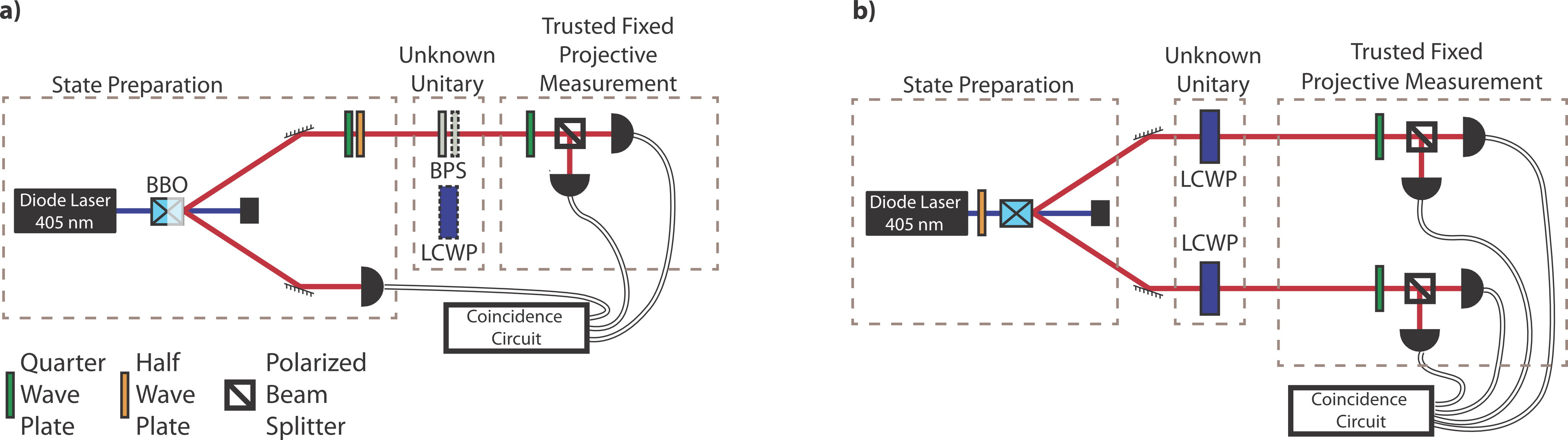
Figure 1: Experimental scheme: a) A single-qubit state is prepared, unknown unitary operations are implemented using BPSs or an LCWP and the state is measured using a trusted, fixed measurement; b) An entangled two-qubit state is prepared, unknown local unitary operations are implemented using LCWPs and the two-qubit state is measured using a trusted, fixed measurement.

For the trusted, fixed projector, we chose $\hat{\mu}_{0}=|R\rangle\mbox{}\langle R|$, implemented with a quarter-wave plate and a polarizing beamsplitter, followed by coincidence-counting, as shown in Fig. 1 a). To change the measurement basis, a unitary operation was applied to the state prior to measurement, implemented using either one or two identical pieces of a birefringent polymer sheet (BPS). The BPS is an optical element that alters the polarization state of light in the same way as a wave-plate, with the crucial difference that the retardance of the BPS is not known. The effect of the BPS on the state of the photon can be described by $\hat{R}_{\phi}(\alpha)$ given in (6), where $\alpha$ is the retardance of the BPS, $\varphi$ is the alignment of the BPS’s optical axis with respect to the polarization of the light, and $\hat{\sigma}_{i}$ are in the $|R\rangle/|L\rangle$ basis. Using different alignments of the BPS, we constructed the following operators $\hat{\mu}_{j}(\alpha)=\hat{U}_{j}(\alpha)^{\dagger}\hat{\mu}_{0}\hat{U}_{j}(\alpha)$ using different implementations of $\hat{U}_{j}(\alpha)$:

$$\hat{U}_{0}(\alpha) = \hat{\sigma}_{0}\,,$$ (22)

$$\hat{U}_{1}(\alpha) = \hat{R}_{0}(\alpha)\,,$$ (23)

$$\hat{U}_{2}(\alpha) = \hat{R}_{\frac{\pi}{2}}(\alpha)\,,$$ (24)

$$\hat{U}_{3}(\alpha) = \hat{R}_{\pi}(2\alpha)\,,$$ (25)

$$\hat{U}_{4}(\alpha) = \hat{R}_{\frac{3\pi}{2}}(2\alpha)\,.$$ (26)

Note that rotations of $2\alpha$ were required to satisfy the linear-independence condition on (3). These rotations were realized with a double-pass through the BPS—the sheet was cut in half and the pieces placed in succession. The beam passed through sections of the pieces that were within close proximity before partition, to ensure consistency in the birefringence. One piece was then removed to perform rotations of $\alpha$, before removal of the remaining piece to measure $\hat{\mu}_{0}$. This measurement sequence eliminated the need for realignment between measurements.

In this particular linear-optical implementation of the scheme, both output ports of the PBS are easily accessible. We therefore measured the complimentary projectors, $\hat{\mu}_{j}^{\prime}(\alpha)=\hat{U}_{j}(\alpha)^{\dagger}\hat{\mu}_{0}^{\prime}\hat{U}_{j}(\alpha)$ where $\hat{\mu}_{0}^{\prime}=|L\rangle\mbox{}\langle L|$, to determine $\mathcal{N}_{j}$.

Using this method, SCT was performed on 14 states: six that lie at the ends of the three axes and eight other states defined by all combinations of $\theta=\pm\frac{\pi}{4}$ and $\phi=\{\pm\frac{\pi}{4},\pm\frac{3\pi}{4}\}$ where $|\psi\rangle~=~\cos\left(\frac{\theta}{2}\right)|R\rangle~+~\mathrm{e}^{i\phi}\sin\left(\frac{\theta}{2}\right)|L\rangle$. Each state was reconstructed using the maximum-likelihood estimation method described in Section 2.3 in conjunction with the YALMIP solver [32].

For comparison, standard tomography (ST) was also performed on each of the states. ST required fewer projectors $\hat{\mu}_{j}=\hat{U}_{j}^{\dagger}\hat{\mu}_{0}\hat{U}_{j}$, given by the unitary operators:

$$\hat{U}_{0} = \hat{\sigma}_{0}$$ (27)

$$\hat{U}_{1} = R_{0}\left(\frac{\pi}{2}\right)$$ (28)

$$\hat{U}_{2} = R_{\frac{\pi}{2}}\left(\frac{\pi}{2}\right)\,,$$ (29)

and their complimentary projectors, $\hat{\mu}_{j}^{\prime}=\hat{U}_{j}^{\dagger}\hat{\mu}_{0}^{\prime}\hat{U}_{j}$ where $\hat{\mu}_{0}^{\prime}=|L\rangle\mbox{}\langle L|$. We used the fidelity $F=\mathrm{Tr}[\sqrt{\sqrt{\hat{\rho}_{\textsc{st}}}\hat{\rho}_{\textsc{sct}}\sqrt{\hat{\rho}_{\textsc{st}}}}]^{2}$ to characterize the success of SCT, where $\hat{\rho}_{\textsc{st}}$ and $\hat{\rho}_{\textsc{sct}}$ are the density operators reconstructed using ST and SCT respectively. We achieved an average fidelity $\bar{F}=0.99\pm 0.01$ and determined the retardance of the BPS (at $405nm$) to be $\alpha=0.58\pm 0.03$ (close to $\pi/6$). Individual fidelities for each state are shown in Fig. 2 a).

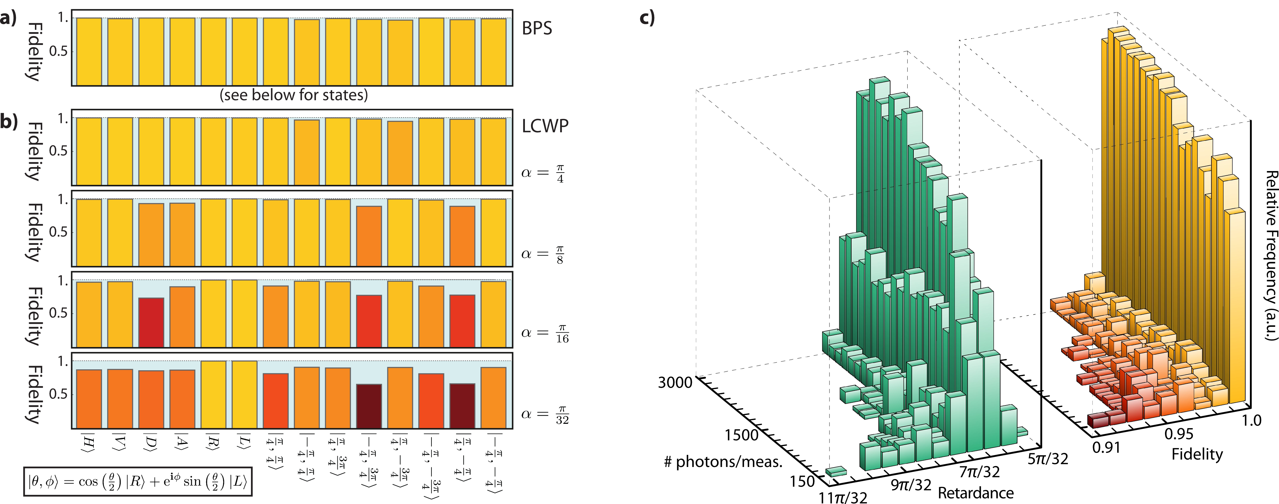
Figure 2: Single-shot fidelity between SCT and ST for 14 states distributed on the Bloch sphere, using: a) a birefringent polymer sheet (BPS) as the uncalibrated wave plate; and b) using a liquid crystal wave plate (LCWP) set to different values of the retardance $\alpha$. c) Histogram showing the predicted retardance and the fidelity between SCT and ST, for 100 runs of SCT with varying numbers of total photons collected (and hence levels of counting error). All used $|\psi\rangle=|H\rangle$ and the BPS.

3.2 Dependence on retardance

To determine the effectiveness of SCT as a function of the retardance, we repeated the experiment using BolderVision Optik liquid crystal wave plates (LCWP), as shown in Fig. 1 a). In an LCWP, the birefringence is a function of the applied voltage, allowing for the retardance to be set arbitrarily. A single LCWP was used to implement rotations of $\alpha$ and $2\alpha$ using different voltage settings. Fidelities for different setting of $\alpha$ are shown in Fig. 2 b). The average fidelity decreases with the size of the retardance. The fidelity for states $|\psi\rangle=|R\rangle$ and $|\psi\rangle=|L\rangle$ always remains close to unity. This is a consequence of our choice of measurement projectors. Using the LCWP, we find a slightly lower average fidelity with a greater spread over the different states, even for values of $\alpha$ larger than that of the BPS. We attribute this to errors associated with the non-linear dependence of the retardance on the voltage passed through the LCWP. This influences how accurately $2\alpha$ can be set with respect to $\alpha$.

3.3 Dependence on noise

To investigate the dependence of the fidelity on the amount of noise, we performed SCT on the state $|\psi\rangle=|H\rangle$ using a retardance $\alpha=\pi/32$. The noise scales inversely with the square root of the number of counts and by collecting from 150 to 3000 photons we varied the noise between roughly $1\%$ and $10\%$. For each noise setting, SCT was repeated 100 times. The resulting fidelities and predicted retardances are presented in Fig. 2 c). Notice that the majority of predicted fidelities and retardances correspond to the actual values. However, recall that the likelihood function can have multiple local minima, making it possible for the maximum likelihood algorithm to converge to a state and retardance that do not correspond to the actual state. This shows up in the high-noise, or low photon-number, region and can be seen as a small bump in the fidelity histogram (and to a lesser extent in the retardance histogram) in Fig. 2 c). As the noise decreases, only high-fidelity results corresponding to the actual state and retardance remain. Fig. 3 shows the distribution of states on the Bloch sphere as predicted by SCT for high and low noise amounts. The darker red cluster of states in Fig. 3 a) also correspond to a local minimum in the likelihood function.

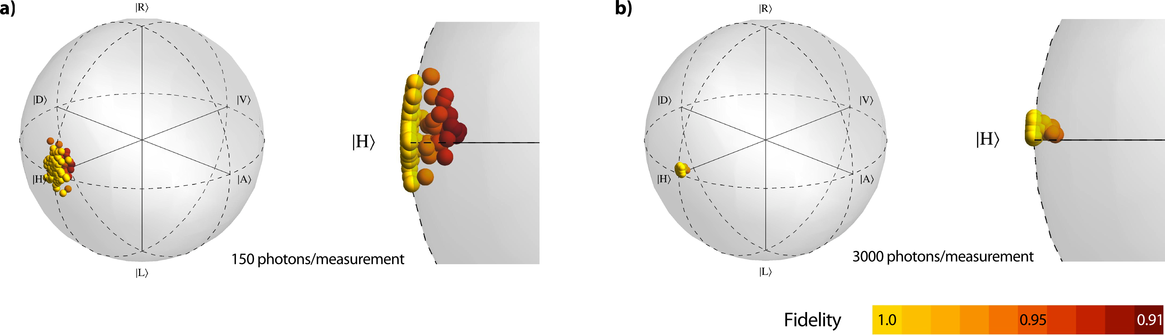
Figure 3: Distribution of states on the Bloch sphere as predicted by SCT for: a) high noise; and b) low noise. Notice the darker red cluster of states in Fig. a), which corresponds to a local minimum in the likelihood function. There are 100 states shown in each sphere.

3.4 Entangled qubits

For multi-qubit tomography, entangled two-qubit states, $|\psi\rangle=a|HH\rangle+b|VV\rangle$, were prepared using two $1mm$ long type-I down-conversion BBO crystals with optical axes aligned in perpendicular planes [33] pumped by a $405nm$ diode laser, as shown in Fig. 1 b). The parameters $a$ and $b$ which characterise the state were tuned by changing the polarization of the pump beam with a HWP. LCWPs in each arm, implemented the unknown unitary operations, followed by detection of $\hat{\mu}_{0}=|R\rangle\mbox{}\langle R|$ in both modes. For this two-qubit experiment, LCWPs were chosen over the BPSs due to realignment issues that accompany the insertion (as opposed to removal) of optical elements in the beam-path. The concurrence [34] for states reconstructed using SCT and ST, as well as the fidelity between the two, are shown for a variety of entangled states in Table 1.

$C_{\textsc{SCT}}$	$C_{\textsc{ST}}$	$F$
$0.905\pm 0.005$	$0.927\pm 0.003$	$0.968\pm 0.0028$ *
$0.566\pm 0.005$	$0.562\pm 0.005$	$0.978\pm 0.0012$
$0.337\pm 0.005$	$0.328\pm 0.004$	$0.977\pm 0.0032$
$0.004\pm 0.004$	$0.010\pm 0.003$	$0.989\pm 0.0015$ **

Table 1: The concurrence [34] as predicted by both tomographic techniques and fidelity between the two reconstructions for states with different degrees of entanglement. Density matrices for * and ** are shown in Figure 4 a) and b) respectively. Error bars were determined by using Poissonian noise in a Monte Carlo simulation

Fig. 4 shows density matrices for the most- and least-entangled states. The retardances were determined to be $\alpha_{1}=0.810\pm 0.009$ and $\alpha_{2}=0.760\pm 0.006$, compared with the known value $\alpha=\pi/4\approx 0.785$.

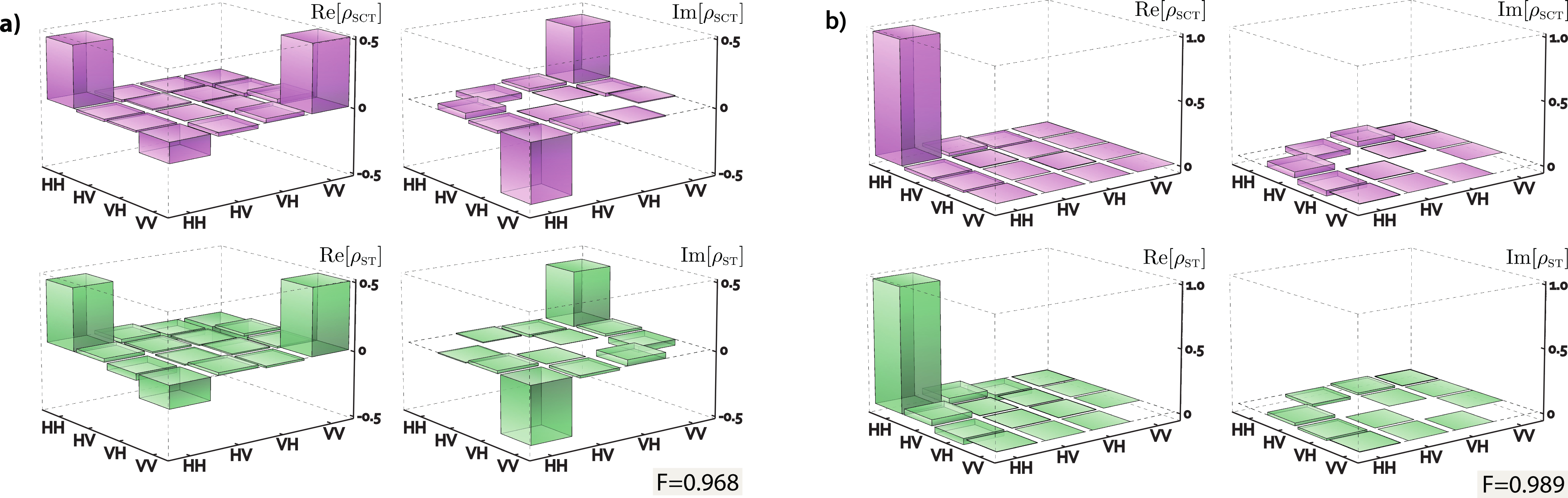
Figure 4: Comparison between density matrices reconstructed using SCT and ST: a) $F=0.968\pm 0.0028$; b) $F=0.989\pm 0.0015$. For concurrences and other fidelities, refer to Table 1.

4 Potential applications to photosynthetic systems

In this section, we give some detail about how this technique may be applied to performing quantum state tomography on biological molecules, such as chromophores in photosynthetic systems, where the transition dipole moment and its orientation are not known with high accuracy.

4.1 Unitary operation

Consider a molecule with two states of interest—the ground state $|g\rangle$ and the excited state $|e\rangle$—that undergoes an interaction with an EM field, e.g. a laser pulse, given by the interaction Hamiltonian

$$\hat{H}=\hat{\mathbf{d}}\cdot E(t)=\vec{d}_{eg}\cdot E(t)|e\rangle\mbox{}\langle g|+\vec{d}_{ge}\cdot E(t)^{*}|g\rangle\mbox{}\langle e|\,,$$ (30)

where $E(t)$ is the electric field, $\hat{\mathbf{d}}$ is the transition dipole moment operator and $\vec{d}_{eg}=\mbox{}\langle e|\hat{\mathbf{d}}|g\rangle=d^{*}_{ge}$. An ultra-fast pulse with a carrier frequency $\omega_{c}$ can be described by $E(t)=\mathcal{E}(t)\mathrm{e}^{i\omega_{c}{t}}\vec{e}+\mathrm{h.c.}$, where $\mathcal{E}(t)$ is the temporal profile of the pulse and $\vec{e}$ is the polarization vector. Under the rotating wave approximation, we can write the Hamiltonian in the interaction picture as

$$\hat{H}=(\vec{d}_{eg}\cdot\vec{e})\mathcal{E}(t)\mathrm{e}^{i(\omega_{c}-\omega_{e})t}|e\rangle\mbox{}\langle g|+(\vec{d}_{eg}\cdot\vec{e})^{*}\mathcal{E}(t)^{*}\mathrm{e}^{-i(\omega_{c}-\omega_{e})t}|g\rangle\mbox{}\langle e|\,,$$ (31)

where $\omega_{e}$ is the $|g\rangle\rightarrow|e\rangle$ transition energy. The unitary governing the interaction is given by

$$\hat{U}_{j}(\alpha)=\mathrm{e}^{-\frac{i}{\hbar}\int dt\hat{H}(t)}=\mathrm{e}^{-i\left(\mathrm{Re}[\Omega]\hat{\sigma}_{x}+\mathrm{Im}[\Omega]\hat{\sigma}_{y}\right)/2}=\mathrm{e}^{-i\nu\alpha\left(\cos(\varphi)\hat{\sigma}_{x}+\sin(\varphi)\hat{\sigma}_{y}\right)/2}\,,$$ (32)

where $\Omega=\frac{2}{\hbar}(\vec{d}_{eg}\cdot\vec{e})\int dt\mathcal{E}(t)\mathrm{e}^{i(\omega_{c}-\omega_{e})t}$ and

$$\nu = \frac{2}{\hbar}\left|\int dt\mathcal{E}(t)\mathrm{e}^{i(\omega_{c}-\omega_{e})t}\right|\,,$$ (33)

$$\alpha = (\vec{d}_{eg}\cdot\vec{e})\,,$$ (34)

$$\varphi = \mathrm{arg}\left(\int dt\mathcal{E}(t)\mathrm{e}^{i(\omega_{c}-\omega_{e})t}\right)\,.$$ (35)

Comparing with (6), we can see that (32) constitutes a rotation of angle $\nu\alpha$, where $\varphi$—determined by the relative phase of $\mathcal{E}(t)$—defines the rotation axis. Notice from (33) that $\nu$ is linearly proportional to the square root of the intensity of the pulse at the transition frequency. We can therefore execute rotations of $2\alpha$ by changing the intensity of the pulse, without any knowledge of $\vec{d}_{eg}\cdot\vec{e}$.

4.2 Projective measurement

We can perform a measurement corresponding to the operator

$$\hat{\mu}_{0}=|e\rangle\mbox{}\langle e|\,,$$ (36)

by preparing multiple copies of the state and performing statistics on the number of photons emitted. A molecule in the excited state will—on a long enough time-scale—emit a photon, while one in the ground state will not; a molecule in a superposition of ground and excited states $a|g\rangle+b|e\rangle$ will emit a photon with probability $|b|$. The measurement statistics will be given by

$$n_{j}=\mathcal{N}_{j}\mathrm{Tr}[\hat{U}_{j}(\alpha)\hat{\rho}\hat{U}_{j}(\alpha)^{\dagger}\hat{\mu}_{0}]\,,$$ (37)

where $\hat{U}_{j}(\alpha)$ is given in (32) and $\mathcal{N}_{j}$ depends on the solid angle of the detector, the position of the detector with respect to the dipole moment of the molecule and losses.

Measurement statistics can be collected either by repeated preparation and measurement of a single molecule, recently demonstrated by Hildner et al. [35, 36], which is analogous to the linear-optical implementation discussed above; or by preparing an ensemble of molecules in the same state and measuring the fluorescence of the sample, where the time-integrated intensity of the emitted light is directly proportional to the number of photons. An open question is whether it will be possible for the self-calibrating technique to compensate for an ensemble of randomly oriented molecules. This is currently being investigated.

In principle, the extension to multiple entangled molecules should be straightforward: even if individual molecules can not be spatially isolated, independent rotations on each qubit could be executed with appropriately shaped pulses, as long as there are different transition energies for each molecule. However, in the case of coupled molecules, there are technical difficulties associated with addressing the transition energies of the individual molecules—the system rather absorbs light at the eigen-energies of the coupled Hamiltonian. In this case, a system of two coupled two-level systems can be approximated as a three-level system (where the fourth level is typically disregarded). Self-calibrating quantum state tomography of coupled two-level system will require an extension of our formalism to a three-dimensional Hilbert space. This is also currently being investigated.

5 Conclusion

In conclusion, we have introduced and demonstrated a technique for performing quantum state tomography of multi-qubit systems which does not rely on complete knowledge of the unitary operation used to change the measurement basis. Our technique characterizes the state of interest with high fidelity as well as recovering the unknown unitary operation. We find that in the context of QST of polarization-encoded qubits, it is possible to do away with a well-calibrated half-wave plate and replace it with an inexpensive uncharacterized piece of birefringent material.

A future extension of this work will attempt to incorporate unknown rotation axes and non-unitary transformations, such as those that introduce noise to the system, thereby reducing the purity of the state by an unknown amount.

We anticipate our method to be applicable to quantum state tomography of systems that do not have well-characterized transition dipole moments, such as biological molecules like those found in photosynthetic systems, as well as systems that experience variability during the fabrication process, such as colloidal quantum dots.

AMB, AD and DFVJ thank DARPA (QuBE) for support. DHM, LAR and AMS thank NSERC, CIFAR and QuantumWorks for support. We also thank Xingxing Xing for the serendipitous discovery of the birefringence of his smartphone screen protector.

References

References

- [1] Pieter Kok, W. J. Munro, Kae Nemoto, T. C. Ralph, Jonathan P. Dowling, and G. J. Milburn. Linear optical quantum computing with photonic qubits. Rev. Mod. Phys., 79(1):135, 2007.
- [2] Andrew M. Childs and Wim van Dam. Quantum algorithms for algebraic problems. Rev. Mod. Phys., 82:1–52, Jan 2010.
- [3] M. A. Nielsen and I. L. Chuang. Quantum computation and quantum information. Cambridge University Press, Cambridge, 2000.
- [4] C. H. Bennett and G. Brassard. Quantum Cryptography: Public Key Distribution and Coin Tossing. In Proceedings of IEEE International Conference on Computers, Systems and Signal Processing, pages 175–179, New York, 1984. IEEE. Bangalore, India, December 1984.
- [5] Daniel F. V. James, Paul G. Kwiat, William J. Munro, and Andrew G. White. Measurement of qubits. Phys. Rev. A, 64:052312, Oct 2001.
- [6] J. B. Altepeter, D. F. V. James, and P. G. Kwiat. Qubit Quantum State Tomography, chapter 4. Springer, 2004.
- [7] J. Benhelm, G. Kirchmair, C. F. Roos, and R. Blatt. Experimental quantum-information processing with 43ca+ ions. Phys. Rev. A, 77:062306, Jun 2008.
- [8] Gregory S. Engel, Tessa R. Calhoun, Elizabeth L. Read, Tae-Kyu Ahn, Tomas Mancal, Yuan-Chung Cheng, Robert E. Blankenship, and Graham R. Fleming. Evidence for wavelike energy transfer through quantum coherence in photosynthetic systems. Nature, 446(7137):782–786, 04 2007.
- [9] Elisabetta Collini, Cathy Y. Wong, Krystyna E. Wilk, Paul M. G. Curmi, Paul Brumer, and Gregory D. Scholes. Coherently wired light-harvesting in photosynthetic marine algae at ambient temperature. Nature, 463(7281):644–647, 02 2010.
- [10] Philippe Guyot-Sionnest. Colloidal quantum dots. Comptes Rendus Physique, 9(8):777 – 787, 2008.
- [11] Joel Yuen-Zhou and Alan Aspuru-Guzik. Quantum process tomography of excitonic dimers from two-dimensional electronic spectroscopy. I. general theory and application to homodimers. The Journal of Chemical Physics, 134(13):134505, 2011.
- [12] Joel Yuen-Zhou, Jacob J. Krich, Masoud Mohseni, and Alán Aspuru-Guzik. Quantum state and process tomography of energy transfer systems via ultrafast spectroscopy. Proceedings of the National Academy of Sciences, 108(43):17615–17620, 2011.
- [13] Koji Maruyama, Daniel Burgarth, Akihito Ishizaki, K. Birgitta Whaley, and Takeji Takui. Hamiltonian tomography of dissipative systems under limited access: A biomimetic case study. arXiv:1111.1062v2 [quant-ph], 2011.
- [14] J. B. Altepeter, E. R. Jeffrey, P. G. Kwiat, S. Tanzilli, N. Gisin, and A. Acín. Experimental methods for detecting entanglement. Phys. Rev. Lett., 95:033601, Jul 2005.
- [15] Alexander Ling, Kee Pang Soh, Antía Lamas-Linares, and Christian Kurtsiefer. Experimental polarization state tomography using optimal polarimeters. Phys. Rev. A, 74:022309, Aug 2006.
- [16] R. B. A. Adamson, L. K. Shalm, M. W. Mitchell, and A. M. Steinberg. Multiparticle state tomography: Hidden differences. Phys. Rev. Lett., 98:043601, Jan 2007.
- [17] Jaroslav Řeháček, Zdeněk Hradil, E. Knill, and A. I. Lvovsky. Diluted maximum-likelihood algorithm for quantum tomography. Phys. Rev. A, 75:042108, Apr 2007.
- [18] Mark D. de Burgh, Nathan K. Langford, Andrew C. Doherty, and Alexei Gilchrist. Choice of measurement sets in qubit tomography. Phys. Rev. A, 78:052122, Nov 2008.
- [19] R. B. A. Adamson, P. S. Turner, M. W. Mitchell, and A. M. Steinberg. Detecting hidden differences via permutation symmetries. Phys. Rev. A, 78:033832, Sep 2008.
- [20] Mattego G. A. Paris. Quantum estimation for quantum technology. International Journal of Quantum Information, 7(1):125–137, 2009.
- [21] R. B. A. Adamson and A. M. Steinberg. Improving quantum state estimation with mutually unbiased bases. Phys. Rev. Lett., 105:030406, Jul 2010.
- [22] J. Nunn, B. J. Smith, G. Puentes, I. A. Walmsley, and J. S. Lundeen. Optimal experiment design for quantum state tomography: Fair, precise, and minimal tomography. Phys. Rev. A, 81:042109, Apr 2010.
- [23] Yu. I. Bogdanov, G. Brida, M. Genovese, S. P. Kulik, E. V. Moreva, and A. P. Shurupov. Statistical estimation of the efficiency of quantum state tomography protocols. Phys. Rev. Lett., 105:010404, Jul 2010.
- [24] Z. E. D. Medendorp, F. A. Torres-Ruiz, L. K. Shalm, G. N. M. Tabia, C. A. Fuchs, and A. M. Steinberg. Experimental characterization of qutrits using symmetric informationally complete positive operator-valued measurements. Phys. Rev. A, 83:051801, May 2011.
- [25] Koichi Yamagata. Efficiency of quantum state tomography for qubits. International Journal of Quantum Information, 9(4):1167–1183, 2011.
- [26] Giorgio Brida, Ivo P. Degiovanni, Angela Florio, Marco Genovese, Paolo Giorda, Alice Meda, Matteo G. A. Paris, and Alexander P. Shurupov. Optimal estimation of entanglement in optical qubit systems. Phys. Rev. A, 83:052301, May 2011.
- [27] M. Asorey, P. Facchi, G. Florio, V.I. Man’ko, G. Marmo, S. Pascazio, and E.C.G. Sudarshan. Robustness of raw quantum tomography. Physics Letters A, 375(5):861 – 866, 2011.
- [28] Yu. I. Bogdanov, G. Brida, I. D. Bukeev, M. Genovese, K. S. Kravtsov, S. P. Kulik, E. V. Moreva, A. A. Soloviev, and A. P. Shurupov. Statistical estimation of the quality of quantum-tomography protocols. Phys. Rev. A, 84:042108, Oct 2011.
- [29] Yong Siah Teo, Huangjun Zhu, Berthold-Georg Englert, Jaroslav Řeháček, and Zden ěk Hradil. Quantum-state reconstruction by maximizing likelihood and entropy. Phys. Rev. Lett., 107:020404, Jul 2011.
- [30] Yong Siah Teo, Bohumil Stoklasa, Berthold-Georg Englert, Jaroslav Řeháček, and Zden ěk Hradil. Incomplete quantum state estimation: A comprehensive study. Phys. Rev. A, 85:042317, Apr 2012.
- [31] E. Bocquillon, C. Couteau, M. Razavi, R. Laflamme, and G. Weihs. Coherence measures for heralded single-photon sources. Phys. Rev. A, 79:035801, Mar 2009.
- [32] J. Lofberg. Yalmip: a toolbox for modeling and optimization in matlab. In Computer Aided Control Systems Design, 2004 IEEE International Symposium on, pages 284 –289, sept. 2004.
- [33] Paul G. Kwiat, Edo Waks, Andrew G. White, Ian Appelbaum, and Philippe H. Eberhard. Ultrabright source of polarization-entangled photons. Phys. Rev. A, 60:R773–R776, Aug 1999.
- [34] William K. Wootters. Entanglement of formation of an arbitrary state of two qubits. Phys. Rev. Lett., 80:2245–2248, Mar 1998.
- [35] Richard Hildner, Daan Brinks, and Niek F. van Hulst. Femtosecond coherence and quantum control of single molecules at room temperature. Nat Phys, 7(2):172–177, 02 2011.
- [36] Richard Hildner, Daan Brinks, Fernando D. Stefani, and Niek F. van Hulst. Electronic coherences and vibrational wave-packets in single molecules studied with femtosecond phase-controlled spectroscopy. Phys. Chem. Chem. Phys., 13:1888–1894, 2011.