Unstable electromagnetic modes in strongly magnetized plasmas

Abstract

The electromagnetic modes possibly unstable in strongly magnetized plasmas are identified. The regime where this instability might stand out compared to the incoherent electron-cyclotron radiation is explored. These modes are relevant to the inertial confinement fusion and the gamma ray burst.

I Introduction

The magnetic field is ubiquitous in plasmas. The plasma interaction with the magnetic field often determines its dynamical behavior (Fleming et al., 2000; Biskamp, 1986; Fishman and Meegan, 1995; Nakar, 2007; Innes et al., 1997). In particular, the magnetic field could convert the electron kinetic energy into the collective photons, as in the magnetron or the gyrotron (Bratman et al., 2009; Glyavin et al., 2008) and the free electron laser (FEL) (Malkin and Fisch, 2007; Son and Ku, 2009; Son et al., 2010). In the FEL, a relativistic electron beam gets periodically accelerated amplifying coherent electromagnetic (E&M) waves. The resulting lasers have various applications. One natural question would be whether the electron thermal gyro-motion in the magnetic field, not the specifically designed population-inverted plasma state, can excite an analogous process.

In this letter, we examine the instability of collective E&M waves arising from the electron thermal gyro-motion. The analysis of the electron motion in the presence of a strong magnetic field leads to a theoretical framework similar to that of the Landau damping (Son and Ku, 2009; Son and Moon, 2012), which reveals that there could exist numerous unstable E&M modes in relativistic plasmas. Our theory is similar to the well-known electron maser theory (Chu, 2011; Treumann, 2006), but our theory deals with the long time limit while the previous researches mainly focus on the short time limit, which will be discussed in detail at the end of Sec. (4). We identify the regime where the coherent radiation from this instability might be more intense than the incoherent cyclotron radiation. Various implications of our study on the astrophysical and laboratory plasmas are discussed, including the short gamma ray burst (Nakar, 2007), the non-inductive current drive (Malkin and Fisch, 2007; Son and Fisch, 2005) and the soft x-ray generation in the inertial confinement fusion (Tabak et al., 1994).

This paper is organized as follows. In Sec. (2), the theory of the instability is developed based on the Landau damping theory for the non-relativistic plasmas. In Sec. (3), the fully relativistic theory is developed. This section is the major result of this paper. In Sec. (4), we identify the instability inherent in the relativistic plasmas. In Sec. (5), we discuss the implications of our results.

II Landau theory: Non-relativistic electrons

In this section, we consider the non-relativistic plasma. While we will conclude that the theory developed in this section is inadequate, the intuition derived from this development is useful for the fully relativistic theory in the next section. We start with a non-relativistic electron under the magnetic field $\mathbf{B}_{0}=B_{0}\hat{z}$. The equation of motion is

$$m_{e}\frac{d\mathbf{v}}{dt}=-e\left(\mathbf{E}_{0}+\frac{\mathbf{v}}{c}\times\mathbf{B}_{0}\right)\mathrm{,}$$

where $m_{e}$ ($e$) is the electron mass (charge), $\mathbf{E}_{0}=0$, $\mathbf{v}$ is the electron velocity, and $c$ is the speed of light. The zeroth-order solution is $v^{(0)}_{x}(t)=v_{p}\cos(\omega_{ce}t+\phi_{0})$, $v^{(0)}_{y}(t)=-v_{p}\sin(\omega_{ce}t+\phi_{0})$ and $v^{(0)}_{z}(t)=v_{0z}$, where $\omega_{ce}=eB_{0}/m_{e}c$, $v_{p}$ is the constant perpendicular velocity, and $\phi_{0}$ is the initial phase angle. Now, assume that this electron interacts with a linearly polarized E&M wave propagating in the positive $z$-direction: $E_{x}(z,t)=E_{1}\cos(kz-\omega t)$, $E_{y}=E_{z}=0$, $B_{y}(z,t)=E_{1}(ck/\omega)\cos(kz-\omega t)$, and $B_{x}=B_{z}=0$. The first order linearized equation is

$$m_{e}\frac{d\mathbf{v}^{(1)}}{dt}=-e\left[\mathbf{E}+\frac{\mathbf{v}^{(0)}}{c}\times\mathbf{B}\right]-e\frac{\mathbf{v}^{(1)}}{c}\times\mathbf{B}_{0}\mathrm{.}$$

Expanding the momentum equation of the second order in the $z$-direction and averaging it over $\phi_{0}$, we obtain

$$\frac{dv_{z}}{dt}= - \frac{k}{2}\frac{ck}{\omega}\left(\frac{eE_{1}}{m_{e}}\frac{v_{p}}{c}\right)^{2}\left(\frac{\sin(\alpha t)}{\alpha^{2}}-\frac{\cos(\alpha t)}{\alpha}t\right)$$ (1)

$$+ \left(\frac{eE_{1}}{m_{e}}\right)^{2}\frac{1-\beta_{\parallel}}{c}\left(\frac{\sin(\alpha t)}{\alpha}\right)\mathrm{,}$$

where $\alpha=kv_{0z}-\omega+\omega_{ce}$ and $\beta_{\parallel}=v^{(0)}_{z}/c$. Eq. (1) is exact to the second order in $E_{1}$. The first and the second term of the right hand side are from $(\mathbf{v}^{(0)}/c)\times\mathbf{B}$ and the third term is from $(\mathbf{v}^{(1)}/c)\times\mathbf{B}_{0}$ in Eq. (II). The resonance condition, $\alpha=0$, leads to $\omega-kv_{0z}=\omega_{ce}$, and the resonance electron velocity is $v_{r}=(\omega-\omega_{ce})/k$. Note that $v_{r}$ is positive (negative) if $\omega>\omega_{ce}$ ($\omega<\omega_{ce}$).

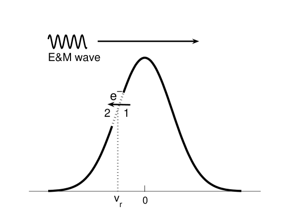
Figure 1: An electron emits a photon in the positive $z$-direction as it transitions from 1 to 2. See more details in the text.

Eq. (1) shares similarity with the Landau damping analysis for a Langmuir wave (Stix, 1962; Son and Moon, 2012). From Eq. (1), we obtain the kinetic energy loss rate of electrons over the electron distribution in the limit of $\alpha t>1$ (Stix, 1962):

$$\frac{d\epsilon}{dt}=\frac{\pi}{2}\frac{E_{x}^{2}}{4\pi}\frac{\omega_{pe}^{2}}{k^{2}}\left[\frac{ck}{\omega}\langle\frac{\beta_{\perp}^{2}}{2}\frac{df}{dv}\rangle-\langle\frac{f(v)}{c}(1-\beta_{\parallel})\rangle\right]ck\mathrm{.}$$ (2)

where $\beta_{\perp}^{2}=v_{p}^{2}/c^{2}=(v_{x}^{2}+v_{y}^{2})/c^{2}$, $\beta_{\parallel}=v_{z}/c$, $\omega_{pe}^{2}=4\pi n_{e}e^{2}/m_{e}$ is the plasma frequency, $f$ is the electron distribution function with the normalization of $\int fd^{3}v=1$, and $\langle\rangle$ is the ensemble average with $v_{z}=v_{r}$ or $\langle A\rangle=\int A\delta(v-v_{r})d^{3}v$. By employing the full relativistic equation (Chu, 2011) and taking the appropriate classical limit, we also verify that Eq. (2) is correct in the energy conservation if the exchange of the electron parallel and perpendicular energy with the E&M wave is fully taken into account. It should be noted that this equation of the energy exchange is well-known in the maser theory (Chu, 2011). The case when $v_{r}<0$ also seems contradictory as the E&M wave (the electron) gains (gains) the momentum (the parallel kinetice energy). This can be resolved by considering the perpendicular electron motion. The electron kinetic energy in the perpendicular direction acts as an energy storage, by which the energy difference between the electron kinetic energy in the $z$-direction and the energy gain of the E&M mode can be accounted for. We demonstrate this idea by a single particle simulation (Fig. 2). As the resonant interaction between the electron and the wave progresses, the electron loses the momentum in the $z$-direction and, at the same time, gains the kinetic energy in the same direction. However, simultaneously, the electron loses more energy in the perpendicular direction. The ratio of the perpendicular energy loss to the parallel energy gain is roughly $c/v_{r}$, which is consistent with the momentum and the energy relation in the quantum mechanics; While the electron gains the kinetic energy in the $z$-direction, it loses the energy in the perpendicular direction by transitioning from a higher energy Landau level to a lower one.

Figure 2: The energy of an electron in the presence of the magnetic field and the E&M wave. The magnetic field is 1 T so that $\omega_{ce}=0.025$ THz, and $\omega=ck=1/1.1\ \omega_{ce}$. The intensity of the E&M field is $2\ \mathrm{MW}/\mathrm{cm}^{2}\sec$. An electron has the initial perpendicular energy 80 keV and parallel energy 4.05 keV. The x-axis is the time normalized by $(ck)^{-1}$ and the y-axis is the change in the parallel, perpendicular and total energy of the electron in the unit of keV. In this particular simulation, the electron parallel kinetic energy increases while its total (perpendicular) kinetic energy decreases.

Assuming the energy density of the wave is given as $\epsilon_{w}=\zeta E_{x}^{2}/4\pi$, we arrive at the wave instability growth rate (Landau growth rate) by equation the kinetic energy loss rate to the wave growth rate, $\Gamma\epsilon_{w}=(d\epsilon/dt)$:

$$\Gamma=\frac{1}{\zeta}\frac{\pi}{2}\frac{\omega_{pe}^{2}}{k^{2}}\left[\frac{ck}{\omega}\langle\frac{\beta_{\perp}^{2}}{2}\frac{df}{dv}\rangle-\langle\frac{f(v)}{c}(1-\beta_{\parallel})\rangle\right]ck\mathrm{.}$$ (3)

In the case of a Langmuir wave, no instabilities exist if the electron distribution is peaked at $v=0$ and monotonically decreases with $v$ because the wave always sees the negative slope of the electron distribution at the resonance. However, this is no longer the case for the E&M mode. If $\omega<\omega_{ce}$, $v_{r}$ and $k$ can be of the opposite signs and an amplification of the E&M wave (as well as the damping) can occur. An E&M mode propagating rightward interacts resonantly with the electrons of certain negative velocity (Fig. 1), and extract the momentum from the resonant electrons. The second term on the right-hand side of Eq. (3) is always a damping term, but the first term could be an amplification or a damping depending on the sign of $df/dv$.

If $\zeta$ is positive, Eq. (3) predicts that the E&M wave becomes unstable in a Maxwellian plasma with $T_{e}>m_{e}c^{2}/2$, seemingly contradicting the Gardner’s constraint (Gardner, 1963; Dodin, 2005) which states that a plasma of an isotropic and monotonically decreasing distribution is stable. This apparent contradiction can be resolved with a proper estimation of the free energy in the plasma. If an E&M wave is present in a plasma, the plasma acquires some free energy from the wave oscillation, and the E&M wave can extract this free energy up to the maximum intensity imposed by the Gardner’s constraint. More specifically, let us assume that the electron distribution is Maxwellian for $t<0$, and that an external E&M wave of $E_{x}$ is suddenly turned on at $t=0$. For $t>0$, the electrons acquire an additional kinetic energy of $\delta\epsilon=\zeta E_{x}^{2}/4\pi-\epsilon_{w}=(\zeta-0.5(1+(\omega/ck)^{2}))E_{x}^{2}/4\pi$, where $\epsilon_{w}=(1/8\pi)E_{x}^{2}(1+(\omega/ck)^{2})$ is the E&M field energy density. Let us assume that the E&M wave grows from $E_{x}$ to $E_{fx}$ due to the instability. Then, the free energy drained into the E&M field energy is given as $\delta\epsilon_{w}=0.5(1+(\omega/ck)^{2})(E_{fx}^{2}-E_{x}^{2})/4\pi$. We obtain the maximum wave intensity from the condition $\delta\epsilon_{w}<\delta\epsilon$,

$$E_{fx}^{2}<\frac{2\zeta}{1+\omega^{2}/(ck)^{2}}E_{x}^{2}\mathrm{.}$$ (4)

III Landau theory: Fully Relativistic electrons

While Eq. (3) is mathematically correct, the instability condition for the Maxwellian plasma predicted by the theory is $T_{e}>m_{e}c^{2}/2$, so that the relativistic consideration is necessary. The momentum equation for a relativistic electron is

$$m_{e}\frac{d\gamma\mathbf{v}}{dt}=-e\left[\mathbf{E}+\frac{\mathbf{v}}{c}\times\mathbf{B}\right]-e\frac{\mathbf{v}}{c}\times\mathbf{B}_{0}\mathrm{,}$$ (5)

where $\gamma^{-2}=1-v^{2}/c^{2}$ is the relativistic factor. Following the same steps as in the classical case for a linearly polarized E&M wave but retaining only the resonance term, the electron energy loss rate after the average over the initial phase is

$$\frac{d(\gamma)}{dt} = -\frac{1}{2\gamma c^{2}}\left(\frac{eE_{1}}{m_{e}}\frac{v_{p}}{c}\right)^{2}\Omega\left(\frac{\sin(\alpha t)}{\alpha^{2}}-\frac{\cos(\alpha t)}{\alpha}t\right)$$ (6)

$$+ \frac{1}{\gamma c^{2}}\left(\frac{eE_{1}}{m_{e}}\right)^{2}\frac{\sin(\alpha t)}{\alpha}\left(1-\frac{\beta_{\perp}^{2}}{2}-\frac{ck}{\omega}\beta_{\parallel}\right)\mathrm{,}$$

where $\Omega(\omega,k,\beta_{\parallel})=(c^{2}k^{2}/\omega)(1-\omega\beta_{\parallel}/ck)-\omega_{ce}/\gamma(\beta)$, and $\alpha=kv_{z}-\omega+\omega_{ce}/\gamma$. Eq. (6) is exact to the second order in $E_{1}$. In the regime where the gyro-frequency is very high so that $\alpha t\gg 1$, the following approximation can be used (Stix, 1962):

$$\int\left[\frac{\cos(\alpha t)}{\alpha}g\right]d^{3}\mathbf{x} \cong 0\mathrm{,}$$

$$\int\left[\frac{\sin(\alpha t)}{\alpha^{2}}g\right]d^{3}\mathbf{x} \cong \int\left[\frac{dg}{d\alpha}\pi\delta(\alpha)\right]d^{3}\mathbf{x}\mathrm{,}$$ (7)

$$\int\left[\frac{\sin(\alpha t)}{\alpha}g\right]d^{3}\mathbf{x} \cong \int\left[g\pi\delta(\alpha)\right]d^{3}\mathbf{x}\mathrm{,}$$

where $g$ is a smooth function of the velocity $\mathbf{\beta}=\mathbf{v}/c$, $dg/d\alpha=(\nabla_{\beta}\alpha\cdot\mathbf{\nabla}_{\beta}g/|\mathbf{\nabla}\alpha(\beta)|^{2})$ is the derivative of the $g$ in the direction of the gradient of $\alpha$. Employing the energy conservation, the growth rate of the E&M wave can be obtained by equating the energy growth rate of the E&M wave to the kinetic energy dissipation rate (Stix, 1962)

$$\Gamma\frac{E_{1}^{2}}{8\pi}\cong\langle\frac{d(\gamma)}{dt}m_{e}c^{2}\rangle_{AVG}\mathrm{,}$$ (8)

where $\langle\rangle_{AVG}$ is the ensemble average over the electron distribution. For $\alpha t\gg 1$, the growth rate $\Gamma$ is given from Eqs. (6), (7) and (8) as (Stix, 1962)

$$\Gamma= + \frac{1}{\zeta}\left[\frac{\pi}{2}\frac{\omega_{pe}^{2}}{c^{2}k^{2}}\langle\frac{\mathbf{\nabla}_{\beta}S}{|\mathbf{\nabla}S(\beta)|^{2}}\cdot\mathbf{\nabla}_{\beta}\left(f\frac{\Omega(\omega,k,\beta_{\parallel})}{\gamma}\frac{\beta_{\perp}^{2}}{2}\right)\rangle_{S=0}\right]$$ (9)

$$- \left[\frac{\pi}{2}\frac{\omega_{pe}^{2}}{c^{2}k^{2}}\langle\frac{1-\frac{\beta_{\perp}^{2}}{2}-\frac{ck}{\omega}\beta_{\parallel}}{\gamma}f\rangle_{S=0}\right]ck\mathrm{,}$$

where $\mathbf{\beta}=\mathbf{v}/c$, and $S(\mathbf{\beta})=\beta_{\parallel}-\omega/ck+\omega_{ce}/(ck\gamma(\beta))$, $f$ is the electron distribution with the normalization of $\int fd^{3}\mathbf{\beta}=1$, and $\langle A\rangle_{S=0}=\int\delta(S)Ad^{3}\mathbf{\beta}$ is the integration of the velocity space with the constraint $S=0$. Depending on whether more electrons lose or gain the energy in the resonance boundary $S(\mathbf{\beta})=0$, the growth rate, $\Gamma$ in Eq.(9), could be of either sign. Let us consider the classical limit of Eq. (9), $S\cong\beta_{\parallel}-\omega/ck-\omega_{ce}/ck$ and $\gamma\cong 1$. The resonance boundary is the same as the case in Eq. (3), and Eq. (9) is simplified to

$$\Gamma= + \frac{1}{\zeta}\frac{\pi}{2}\frac{\omega_{pe}^{2}}{k^{2}}\left[\langle\frac{\beta_{\perp}^{2}}{2}\frac{df}{dv}\rangle\right]\Omega$$ (10)

$$- \frac{1}{\zeta}\frac{\pi}{2}\frac{\omega_{pe}^{2}}{k^{2}}\left[\langle\frac{f(v)}{c}(1-\frac{\beta_{\perp}^{2}}{2}-\frac{ck}{\omega}\beta_{\parallel})\rangle\right]ck\mathrm{.}$$

where $\Omega=(c^{2}k^{2}/\omega)(1-\omega\beta_{||}/ck)-\omega_{ce}$. Eqs. (9) and (10) are the major result of our analysis. While Eq. (9) is similar with Eq. (3), there is a crucial difference; at $\omega=ck$, there could be an instability from Eq. (3), which is not the case with Eq. (9). One of the key limitations of Eq. (3) is the fact that the change of the cyclotron resonance frequency due to the change in the relativistic electron mass was not properly taken into account.

As the distribution function described by the Vlasov equation is incompressible in the canonical coordinate of $(p,q)$, the Gardner’s constraint is partially relevant for the relativistic Maxwellian plasmas. Consider an initially isotropic Maxwellian plasma, which has no collective waves at its initial state. In the absence of the E&M waves, the electron kinetic energy is a function of the canonical momentum, and, due to the Gardner’s constraint, an certain amplified E&M wave cannot escape from the plasma if the final plasma has no collective E&M wave. However, a steady-state plasma without any collective wave rarely exists. Let us consider a plasma initially with some collective waves of appreciable energy (more specifically plasmons and photons with $\omega\cong\omega_{pe}$). Noting that the Vlasov equation is compressible in the coordinate of $(r,v)$ and the electron kinetic energy is given as $E=\sqrt{m_{e}^{2}c^{4}+c^{2}(p-eA(r,t)/c)^{2}}$, the Gardner’s constraint no longer applies because the electron kinetic energy is now a function of the wave vector. Some collective E&M waves could be radiated while some other waves still remain in the plasma. Eqs. (9) and (10) suggest that the collective E&M wave is a channel through which the plasma free energy can be drained quickly.

IV Instability

One notable consequence of Eqs. (9) and (10) is that an unstable E&M mode might exist even in Maxwellian plasmas. First, consider the case $ck<\omega$ in the classical limit given in Eq. (10), assuming the electron distribution is an isotropic Maxwellian with the electron thermal velocity $v_{th}$. In contrast to the example given in Fig. 1, the first term on the right-hand side of Eq. (10) is positive if $v_{r}=\omega/k-\omega_{ce}/k>0$. For a positive $v_{r}$, the growth rate is given as

$$\Gamma=\frac{1}{\zeta}\frac{\pi}{2}\frac{\omega_{pe}^{2}}{c^{2}k^{2}}\left(\frac{v_{r}}{c^{2}}|\Omega|-(1-\beta_{th}^{2}-\frac{ck}{\omega}\beta_{r})k\right)f_{\parallel}(v_{r})\mathrm{,}$$ (11)

where $\beta_{th}=v_{th}/c$, $\beta_{r}=v_{r}/c$, and $f_{\parallel}(v)=1/\sqrt{2\pi}v_{th}\exp(-v^{2}/(2v_{th}^{2}))$. The condition for the instability ($\Gamma>0$) is

$$\beta_{r}>\frac{1-\beta_{th}^{2}}{|\Omega|/ck+ck/\omega}\mathrm{.}$$ (12)

For an instability to be appreciable, $f(v_{r})$ should be appreciably large or Eq. (12) should be satisfied near $\beta_{r}\cong\beta_{th}$. The maximum possible growth rate at $v_{r}=v_{th}$ is given roughly as

$$\Gamma_{max}\cong 0.19\times\frac{\omega_{\mathrm{pe}}^{2}}{(ck)^{2}}\Omega\mathrm{,}$$ (13)

where it is assumed that $\zeta\cong 1$. For an anisotropic plasma, the instability condition is

$$\beta_{r}|\Omega|>\left(\frac{v_{\parallel}}{v_{\perp}}\right)^{2}\left[1-\left(\frac{v_{\perp}}{c}\right)^{2}-\frac{ck}{\omega}\frac{v_{r}}{c}\right]\mathrm{,}$$ (14)

where $v_{\parallel}$ ($v_{\perp}$) is the electron thermal velocity in the parallel (perpendicular) direction. If $v_{\parallel}/v_{\perp}\ll 1$, the instability range becomes much wider than the isotropic case, and the maximum growth rate is given as

$$\Gamma_{max}\cong 0.19\times\left(\frac{v_{\perp}}{v_{\parallel}}\right)^{2}\frac{\omega_{\mathrm{pe}}^{2}}{(ck)^{2}}\Omega\mathrm{.}$$ (15)

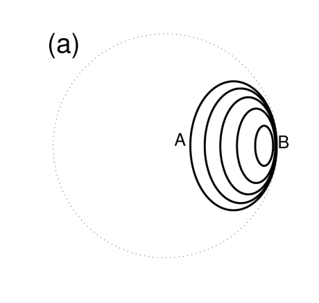
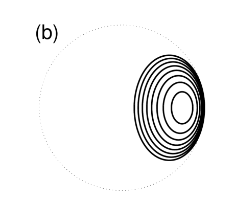
Figure 3: The contours of the resonance boundary ($S(\beta)=0$) of the fully relativistic plasma for the case of $\omega>ck>\omega_{ce}$. (a) $\omega/(ck)=1.1$ and $\omega_{ce}/(ck)$ decreases from 0.9 (the outer-most ellipse) to 0.5 (the inner-most one) by 0.1, and (b) $\omega_{ce}/(ck)=0.9$ and $\omega/(ck)$ increases from 1.04 (the outer-most ellipse) to 1.32 (the inner-most one) by 0.04. Dotted lines are unit circles. The abscissa is $\beta_{\perp}$ and the ordinate is $\beta_{\parallel}$.

For the fully relativistic relation (Eq. (9)), the stability analysis gets more complicated. Here we consider only one case of $\omega>ck>\omega_{ce}$. The Maxwellian electron distribution is given as $f(\beta)\cong\gamma^{3}\exp(-\gamma/T_{e})$, which is the so-called Maxwell-Juttner’s distribution (Bret et al., 2010). When $\gamma_{0}=T_{e}/m_{e}c^{2}>1$, it is peaked at $\gamma=3\gamma_{0}$ with the width of $\delta\beta\cong s/\gamma_{0}^{2}$. Here, we assume that, at the resonance, the derivative of the distribution $f$ is large dominating other terms. Then, Eq. (9) can be simplified to

$$\Gamma= + \frac{1}{\zeta}\left[\frac{\pi}{2}\frac{\omega_{pe}^{2}}{c^{2}k^{2}}\langle\frac{\Omega(\omega,k,\beta_{\parallel})}{\gamma}\frac{\beta_{\perp}^{2}}{2}\frac{\mathbf{\nabla}_{\beta}S\cdot\mathbf{\nabla}_{\beta}f}{|\mathbf{\nabla}S(\beta)|^{2}}\rangle_{S=0}\right]$$ (16)

$$- \left[\frac{\pi}{2}\frac{\omega_{pe}^{2}}{c^{2}k^{2}}\langle\frac{1-\frac{\beta_{\perp}^{2}}{2}-\frac{ck}{\omega}\beta_{\parallel}}{\gamma}f\rangle_{S=0}\right]ck\mathrm{.}$$

Assuming $\beta\cong 1$, the condition $\Gamma>0$ can be recasted as

$$\int_{S=0}\mathbf{d^{3}\beta}\left(\frac{\mathbf{\nabla_{\beta}}S\cdot\mathbf{\nabla_{\beta}}f}{|\nabla S(\mathbf{\beta})|^{2}}\right)\left(\frac{\omega_{ce}}{\gamma ck}+1\right)\left(1-\frac{ck}{\omega}\right)$$

$$>\int_{S=0}\mathbf{d^{3}\beta}f(\beta_{res})\left(1-\frac{ck}{\omega}\beta_{res}\right)\mathrm{.}$$ (17)

When $\omega>ck>\omega_{ce}$, the resonance boundary is of an elliptical shape (Fig. 3). The resonance surface $S$ has the maximum at $\beta_{max}=1/\sqrt{1+(\omega_{ce}/ck)^{2}}$. The necessary condition for the existence of the resonance is $\omega/ck<\beta_{max}+\omega_{ce}/\gamma_{max}$, where $\gamma_{max}=(1-\beta_{max}^{2})^{-1/2}$. If the electron distribution has the relatively high slope near the resonance region ($\gamma_{max}\cong 3T_{e}/m_{e}c^{2}$), Eq. (17) is possible since $|\nabla_{\beta}S|\ll 1$ near the resonance. The growth rate without the gyro-damping term can be estimated, using $\nabla_{\beta}f\cong\gamma^{2}(3-\lambda\gamma)f\mathbf{\beta}$ and $\beta\cong 1$, as

$$\Gamma_{max}\cong\frac{\omega_{\mathrm{pe}}^{2}}{(ck)^{2}}\int\delta(S)\left[\gamma\Omega_{1}(3-\lambda)f\frac{dS/d\beta}{|\nabla_{\beta}S|^{2}}\right]d^{3}\mathbf{\beta}\mathrm{,}$$ (18)

where $(dS/d\beta)=(\mathbf{\beta}\cdot\nabla S)/|\mathbf{\beta}|$.

A similar analysis with Eqs. (1) and (6) is reported in the context of the electron cyclotron maser instability (Chu, 2011); however, the major focus is in the short time growth rate ($\alpha t<1$) when the magnetic field is not intense and/or the electron density is low. In the inertial confinement fusion or the astrophysical dense plasmas, the situation of the magnetic field of giga-gauss and the electron density exceeding $10^{22}\mathrm{cm^{-3}}$ is common, and the Landau damping analysis valid for $\alpha t\gg 1$ should be sought instead of the conventional approach (Chu, 2011; Treumann, 2006); Eqs. (9) and (10) provide a proper estimation of the collective instabilities of dense strongly magnetized plasma. While the instability analysis in this paper focused on Maxwellian plasmas, Eqs. (9) and (10) apply to not only Maxwellian plasmas but also general relativistic strongly magnetized plasmas such as jets, shock regions and accretion disk where the non-Maxwellian electron distribution is common.

An E&M mode from the background noise could grow with the rate given in Eq. (3). This radiation could be more explosive than the incoherent cyclotron radiation. The ratio of the cyclotron radiation power per electron $P$ to the electron kinetic energy is $\Gamma_{ci}=(2P/mv_{p}^{2})=(4/3)(ke^{2}/m_{e}c^{2})\omega$, where the electrons are assumed to be non-relativistic. Using Eq. (13), we arrive at $\Gamma_{max}/\Gamma_{ci}\cong(n_{e}/k^{3})(\Omega/\omega)$. If $\Gamma_{max}/\Gamma_{ci}>1$, the radiation from unstable E&M modes could be more explosive than the cyclotron radiation.

V Conclusion

To summarize, the coherent E&M instabilities of strongly magnetized relativistic electrons are analyzed in the context of the Landau damping theory. Our main results are Eqs. (9) and (10). Our theory based on the long-time scale is relevant with the hard x-ray and the gamma ray generation in the strongly magnetized dense plasmas. In an astrophysical plasma, a strong and large spatial scale magnetic field in the range of $10^{10}-10^{15}$ gauss is often encountered. Its radiation may have to be re-examined in terms of the possible unstable modes identified in our analysis. More specifically, the theory would be relevant with the generation of the soft and the hard x-ray, and the gamma ray (Litvinenko et al., 1997). The complications when applying the above theory to astrophysical plasmas are the relativistic effect and the electron quantum diffraction (Son and Fisch, 2004, 2005; Son et al., 2010; Son and Ku, 2009). One more relevant phenomenon is the non-inductive current drive (Malkin and Fisch, 2007; Son and Fisch, 2005). During the E&M wave amplification, the electrons giving the energy to the E&M wave lose their momentum at an increased rate, as the collision frequency increases compared to the case of no interaction with the E&M wave. This leads to the well-known non-inductive current drive (Malkin and Fisch, 2007; Son and Fisch, 2005).

The authors are thankful to Dr. I. Dodin and Prof. N. J. Fisch for many useful discussions and advice.

References

- Fleming et al. (2000) T. P. Fleming, J. M. Stone, and J. F. Hawley, Apj 530, 464 (2000).
- Biskamp (1986) D. Biskamp, Physics of Fluids 29, 1520 (1986).
- Fishman and Meegan (1995) G. Fishman and C. A. Meegan, Annual review of astronomy and astrophysics 33, 415 (1995).
- Nakar (2007) E. Nakar, Physics Reports 442, 166 (2007).
- Innes et al. (1997) D. E. Innes, B. Inhester, W. I. Axford, and K. Wilhelm, Nature 386, 811 (1997).
- Bratman et al. (2009) V. L. Bratman, Y. L. Kalynov, and V. N. Manuilov, Phys. Rev. Lett. 102, 245101 (2009).
- Glyavin et al. (2008) M. Y. Glyavin, A. G. Luchinin, and G. Y. Golubiatnikov, Phys. Rev. Lett. 100, 105101 (2008).
- Malkin and Fisch (2007) V. M. Malkin and N. J. Fisch, Phys. Rev. Lett. 99, 205001 (2007).
- Son and Ku (2009) S. Son and S. Ku, Phys. Plasmas 17, 010703 (2009).
- Son et al. (2010) S. Son, S. Ku, and S. J. Moon, Phys. Plasmas 17, 114506 (2010).
- Son and Moon (2012) S. Son and S. J. Moon, Phys. Plasmas 19, 063102 (2012).
- Chu (2011) K. R. Chu, Rev. Mod. Phys. 76, 489 (2011).
- Treumann (2006) R. A. Treumann, Astron. Astrophys Rev. 13, 229 (2006).
- Son and Fisch (2005) S. Son and N. J. Fisch, Phys. Rev. Lett. 95, 225002 (2005).
- Tabak et al. (1994) M. Tabak, J. Hammer, M. E. Glinsky, W. L. Kruerand, S. C. Wilks, J. Woodworth, E. M. Campbell, M. J. Perry, and R. J. Mason, Physics of Plasmas 1, 1626 (1994).
- Stix (1962) T. H. Stix, The theory of plasma waves (McGraw-Hill, 1962).
- Gardner (1963) C. S. Gardner, Phys. Fluids 6, 839 (1963).
- Dodin (2005) I. Y. Dodin, Physics Letters A 341, 187 (2005).
- Bret et al. (2010) A. Bret, L. Gremillet, and D. Benisti, Phys. Rev. E 81, 036402 (2010).
- Litvinenko et al. (1997) V. N. Litvinenko, B. Burnham, M. Emamian, N. Hower, J. M. J. Madey, P. Morcombe, P. G. O’Shea, S. H. Park, R. Sachtschale, K. D. Straub, et al., Phys. Rev. Lett. 78, 4569 (1997).
- Son and Fisch (2004) S. Son and N. J. Fisch, Phys. Lett. A 329, 16 (2004).