Effect of dynamical traps on chaotic transport in a meandering jet flow

Abstract

We continue our study of chaotic mixing and transport of passive particles in a simple model of a meandering jet flow [Prants, et al, Chaos 16, 033117 (2006)]. In the present paper we study and explain phenomenologically a connection between dynamical, topological, and statistical properties of chaotic mixing and transport in the model flow in terms of dynamical traps, singular zones in the phase space where particles may spend arbitrary long but finite time [Zaslavsky, Phys. D 168–169, 292 (2002)]. The transport of passive particles is described in terms of lengths and durations of zonal flights which are events between two successive changes of sign of zonal velocity. Some peculiarities of the respective probability density functions for short flights are proven to be caused by the so-called rotational-islands traps connected with the boundaries of resonant islands (including the vortex cores) filled with the particles moving in the same frame and the saddle traps connected with periodic saddle trajectories. Whereas, the statistics of long flights can be explained by the influence of the so-called ballistic-islands traps filled with the particles moving from a frame to frame.

1 Introduction

Chaotic advection of water masses with their physical and biochemical characteristics in quasi two-dimensional geophysical flows in the ocean and atmosphere can be studied within the framework of Hamiltonian dynamics. In a recent paper [1] we have studied chaotic mixing and transport of passive particles in a simple kinematic model of a meandering jet flow motivated by the problem of lateral mixing in the western boundary currents in the ocean. We found all the possible bifurcations of advection equations, described the structure of the phase space (which is the physical space for advected particles), and computed some statistical characteristics of chaotic transport. In the present paper we establish a phenomenological connection between dynamical, topological, and statistical properties of chaotic transport and mixing in the same flow. Specific singular zones in the phase space where particles may spend arbitrary long but finite time (dynamical traps in terminology by Zaslavsky [2]), are responsible for anomalous statistical properties. The dynamical traps, connected with rotational islands and saddle trajectories, are responsible, mainly, for anomalous mixing, whereas those ones, connected with ballistic islands — for anomalous transport. These dynamical traps may have strong impact on transport and mixing in real geophysical jet flows.

 

Methods of the theory of dynamical systems are actively used to describe advection of water (air) masses and their properties in the ocean and atmosphere [1, 14, 13, 15, 16, 26, 3, 4, 5, 6, 7, 17, 18, 19, 20, 21, 32]. The geophysical jet currents, like the Gulf Stream, the Kuroshio, the Antarctic circumpolar current, and others in the ocean and the polar night Antarctic jet in the atmosphere, are robust structures whose form typically changes in space and time in a meander-like way. If advected particles rapidly adjust their own velocity to that of background flow and do not affect the flow properties, then the particles are called passive (scalars, tracers, or Lagrangian particles) and their equation of motion is very simple

$$\frac{d{\mathbf{r}}}{dt}={\mathbf{v}}({\mathbf{r}},t)$$ (1)

where ${\mathbf{r}}=(x,y,z)$ and ${\mathbf{v}}=(u,v,w)$ are the position vector and the particle velocity at a point $(x,y,z)$. If the corresponding Eulerian velocity field is supposed to be regular, the vector Eq. (1) in nontrivial cases is a set of three nonlinear deterministic differential equations whose phase space is a physical space of advected particles. It is well known from dynamical systems theory that solutions of this kind of equations can be chaotic in the sense of exponential sensitivity to small variations in initial conditions and/or control parameters. As to advection equations, it was Arnold [8] who firstly suggested chaos in the field lines (and, therefore, in trajectories) for a special class of three-dimensional stationary flows (so-called ABC flows), and this suggestion has been confirmed numerically by Hénon [9]. In the approximation of incompressible planar flows, the velocity components can be expressed in terms of a stream function [10]: $u=-\partial\Psi/\partial y$ and $v=\partial\Psi/\partial x$. The equations of motion (1) in a two-dimensional incompressible flow have now a Hamiltonian form with the streamfunction $\Psi$ playing the role of a Hamiltonian and the coordinates $(x,y)$ of a particle playing the role of canonically conjugated variables.

Advection of passive particles has been shown to be chaotic in a number of theoretical [4, 5, 6, 7, 1, 14, 13, 15, 16, 17, 26, 32] and laboratory [18, 19, 20, 21] models of geophysical jet currents. In our recent paper [1] (Paper I) we have studied mixing, transport, and chaotic advection in a simple kinematic model of a meandering two-dimensional jet flow with a Bickley zonal velocity profile $u\sim\operatorname{sech}^{2}y$ being motivated by the problem of lateral mixing of water masses (together with salinity, heat, nutrients, pollutants, and other passive scalars) in the western boundary currents in the ocean. We derived advection equations in the frame moving with the phase velocity of a running wave imposed on the Bickley jet, found the stationary points, conditions of their stability, and all the possible bifurcations of these equations which were shown to be autonomous in the co-moving frame. Under a periodic perturbation of the wave amplitude, the phase plane of the chosen model flow has been shown to consist of a central eastward jet, peripheral westward currents, and chains of northern and southern circulations (vortex cores) immersed in a chaotic sea which, in turn, contains islands of regular motion. Statistical properties of chaotic transport of advected particles have been characterized in terms of particle’s zonal flights (any event between two successive changes of the sign of the particle’s zonal velocity $u$). Probability density functions (PDFs) of durations and lengths of flights, computed with a number of very long chaotic trajectories, have been found to be complicated functions with local maxima and fragments with exponential and power-law decays.

The aim of this paper is to study a phenomenological connection between dynamical, topological, and statistical properties of chaotic mixing and transport in the meandering jet flow considered in Paper I and to explain transport properties by phenomenon of the so-called dynamical traps. Following to Zaslavsky [2], the dynamical trap is a domain in the phase space of a Hamiltonian system where a particle (or, its trajectory) can spend arbitrary long finite time, performing almost regular motion, despite the fact that the full trajectory is chaotic in any appropriate sense. In fact, it is the definition of a quasi-trap. Absolute traps, where particles could spend an infinite time, are possible in Hamiltonian systems only with a zero measure set. The dynamical traps are due to a stickiness of trajectories to some singular domains in the phase space, largely, to the boundaries of resonant islands, saddle trajectories, and cantori. There are no classification and description of the dynamical traps. Zaslavsky described two types of dynamical traps in Hamiltonian systems: hierarchical-islands traps around chains of resonant islands [27, 28, 12] and stochastic-layer traps which are stochastic jets inside a stochastic sea where trajectories can spend a very long time [29, 2, 12]. It is expected that classification and description of the most typical dynamical traps would help us to construct kinetic equations which will be able to describe transport properties of chaotic systems including anomalous ones [2, 11, 12].

This paper is organized as follows. We start with advection equations derived in Paper I in the frame of reference moving with the phase velocity of a meander whose amplitude changes in time periodically. We compute in Sec. II PDFs for lengths $x_{f}$ and durations $T_{f}$ of zonal flights for a number of chaotic trajectories and show analytically that all the flights start and finish only inside a strip confined by two curves whose form is defined by the condition $u=0$. Some prominent peaks in statistics of short flights ($|x_{f}|<2\pi$) are proved to be caused by stickiness of trajectories to the boundaries of rotational resonant islands filled with regular particles rotating in the same frame (Sec. III). We call this type of dynamical traps as a rotational-island trap (RIT). In Sec. IV we study dynamical traps connected with periodic saddle trajectories, emerged from saddle points of the unperturbed system (4) under the perturbation (5), and prove numerically that the saddle traps (STs) contribute to the statistics of short flights as well. Another type of islands, ballistic islands (filled with regular particles moving from frame to frame), is proved to contribute to the statistics of long flights ($|x_{f}|\gg 2\pi$) in Sec. V. Both the ballistic-islands trap (BITs) and RITs belong to the class of hierarchical-island traps by the Zaslavsky’s classification.

2 Description of chaotic transport in terms of flights

2.1 Basic features of the flow

We take the following specific stream function as a kinematic model of a meandering jet flow in the laboratory frame of reference:

$$\Psi^{\prime}(x^{\prime},y^{\prime},t^{\prime})=\\ =-\Psi^{\prime}_{0}\tanh{\left(\frac{y^{\prime}-a\cos{k(x^{\prime}-ct^{\prime})}}{\lambda\sqrt{1+k^{2}a^{2}\sin^{2}{k(x^{\prime}-ct^{\prime})}}}\right)},$$ (2)

where the width of the jet is $\lambda$. Meandering is provided by a running wave with the amplitude $a$, the wave-number $k$, and the phase velocity $c$. The normalized streamfunction in the frame moving with the phase velocity is

$$\Psi=-\tanh{\left(\frac{y-A\cos x}{L\sqrt{1+A^{2}\sin^{2}x}}\right)}+Cy,$$ (3)

where $x=k(x^{\prime}-ct^{\prime})$ and $y=ky^{\prime}$ are new scaled coordinates, and $A=ak$, $L=\lambda k$, and $C=c/\Psi^{\prime}_{0}k$ are the control parameters. Equations, governing advection of passive particles (1) in the co-moving frame, are the following:

$$\begin{gathered}\begin{aligned} \dot{x}&=\frac{1}{L\sqrt{1+A^{2}\sin^{2}x}\cosh^{2}\theta}-C,\\ \dot{y}&=-\frac{A\sin x(1+A^{2}-Ay\cos x)}{L\left(1+A^{2}\sin^{2}x\right)^{3/2}\cosh^{2}\theta},\end{aligned}\\ \theta=\frac{y-A\cos x}{L\sqrt{1+A^{2}\sin^{2}x}},\end{gathered}$$ (4)

where dot denotes differentiation with respect to dimensionless time $t=\Psi^{\prime}_{0}k^{2}t^{\prime}$.

In Paper I (for more details see [17]) we have found and analyzed all the stationary points, their stability, and the bifurcations of the equations of motion (4). Being motivated by the problem of mixing and transport of water masses and their properties in oceanic western boundary currents like the Gulf Stream and the Kuroshio, we chose the phase portrait shown in Fig. 1a among all the possible flow regimes. Passive particles can move along stationary (in the co-moving frame) streamlines in a different manner. They can move to the east in the jet ($J$) and to the west in northern and southern (with respect to the jet) peripheral currents ($P$). There are also particles rotating in the northern and southern circulation cells (C) in a periodic way. The northern separatrix connects the saddle points at $x_{s}^{(n)}=2\pi n$ and $y_{s}^{(n)}=L\operatorname{Arcosh}\sqrt{1/LC}+A$ and the southern one connects the saddle points at $x_{s}^{(s)}=(2n+1)\pi$ and $y_{s}^{(s)}=-L\operatorname{Arcosh}\sqrt{1/LC}-A$, where $n=0,\pm 1,\dots$.

Figure 1: (a) Stationary streamfunction of a meandering jet in the co-moving frame (3). The flow is divided into three different regimes: circulations ($C$), jet ($J$), and peripheral currents ($P$). (b) Poincaré section of the perturbed meandering jet in the co-moving frame. The parameters of the steady flow are: the jet’s width $L=0.628$, the meander’s amplitude $A_{0}=0.785$ and its phase velocity $C=0.1168$. The perturbation amplitude and frequency are: $\varepsilon=0.0785$ and $\omega=0.2536.$ (c) Turning points of a single chaotic trajectory on the cylinder $0\leq x\leq 2\pi$ are in a strip confined by two curves (6) with $A=A_{0}\pm\varepsilon$.

As a perturbation, we took in Paper I the simple periodic modulation of the meander’s amplitude

$$A=A_{0}+\varepsilon\cos(\omega t+\phi).$$ (5)

Under the perturbation, there arise resonances between the perturbation frequency $\omega$ and the frequencies $f$ of the particle’s rotation in the circulations $C$. A frequency map $f(x_{0},y_{0})$, computed in Paper I (see Fig. 2 in that paper), shows the values of $f$ for particles with initial positions $(x_{0},y_{0})$ in the unperturbed flow. With a given value of the perturbation frequency and fixed values of the other control parameters, the vortex cores in the circulations survive, stochastic layers appear along the unperturbed separatrix, and the central jet $J$ is a barrier to transport of particles across the jet. In Paper I we fixed the scaled values of the parameters of the unperturbed flow, the jet’s width $L=0.628$, the meander’s amplitude $A_{0}=0.785$ and its phase velocity $C=0.1168$, that are in the range of the realistic values for the Gulf Stream [22, 23], and took the initial phase to be $\phi=\pi/2$. The perturbation frequency $\omega=0.2536$ chosen in Paper I is close to the values of the rotation frequency $f$ of the particles circulating in the inner core of the regions $C$ (see Fig. 2 in Paper I). In Fig. 1 b we show the Poincaré section (for a large number of trajectories) of the meandering jet whose amplitude is modulated with the frequency $w=0.2536$ and the strength $\varepsilon=0.0785$. The vortex cores survive under this perturbation, the stochastic layers appear along the unperturbed separatrix, and a central jet $J$ is a barrier to transport of particles across the jet.

The equations of motion (4) with the perturbation (5) are symmetric under the following transformations: (1) $t\to t$, $x\to\pi+x$, $y\to-y$ and (2) $t\to-t$, $x\to\ -x$, $y\to y$. It implies that the meridional transport (north-south and south-north) is symmetric but the zonal transport (west-east and east-west) is symmetric under a time reversal. Due to these symmetries motion can be considered on the cylinder with $0\leq x\leq 2\pi$ and $y\geq 0$. The part of the phase space with $2\pi n\leq x\leq 2\pi(n+1)$, $n=0,\pm 1,\dots$, is called a frame.

It is convenient to characterize chaotic mixing and transport in terms of zonal flights. A zonal flight is a motion of a particle between two successive changes of signs of its zonal velocity, i. e. the motion between two successive events $\dot{x}=u=0$. Particles (and corresponding trajectories) in chaotic jet flows can be classified in terms of the lengths of flights $x_{f}$ as follows. The trajectories with $|x_{f}|<2\pi$ correspond to the particles moving in the same frame or in neighbor frames. In the global stochastic layer there are particles moving chaotically forever in the same frame but they are of a zero measure. Among the particles with inter-frame motion, there are regular and chaotic ballistic ones. Regular ballistic trajectories can be defined as those which cannot have two flights with $|x_{f}|>2\pi$ in succession. They correspond to particles moving in regular regions of the phase space persisting under the perturbation, (eastward motion in the jet and western motion in the peripheral current) and those moving in the stochastic layer (trajectories belonging to ballistic islands). Typical chaotic trajectories have complicated distributions over the lengths and durations of flights.

In the laboratory frame of reference, all the fluid particles move to the east together with the jet flow and a flight is a motion between two successive events when the particle’s zonal velocity $U$ is equal to the meander’s phase velocity $c$. If $U<c$, the corresponding particle is left behind the meander (it is a western flight in the co-moving frame), if $U>c$, it passes the meander (an eastern flight in the co-moving frame). Short flights with $|x_{f}|<2\pi$ (motion in the same spatial frame in the co-moving frame of reference) correspond to the motion in the laboratory frame when two successive events $U=c$ occur on the space interval less than the meander’s spatial period $2\pi/k$. Ballistic flights between the spatial frames in the co-moving frame with $|x_{f}|>2\pi$ correspond to the motion in the laboratory frame when the particles move through more than one meander’s crest between two successive events $U=c$.

2.2 Turning points

As in Paper I, we will characterize statistical properties of chaotic transport by probability density functions (PDFs) of lengths of flights $P(x_{f})$ and durations of flights $P(T_{f})$ for a number of very long chaotic trajectory. Both regular and chaotic particles may change many times the sign of their zonal velocity $\dot{x}=u$. From the condition $\dot{x}=0$ in Eq. (4), it is easy to find the equations for the curves which are loci of turning points

$$Y_{\pm}(x,A)=\pm L\sqrt{1+A^{2}\sin^{2}{x}}\times\\ \times\operatorname{Arsech}{\sqrt{{LC\sqrt{1+A^{2}\sin^{2}{x}}}}}+A\cos x.$$ (6)

We consider the northern curve, i. e., Eq. (6) with the positive sign. Taking into account that the perturbation has the form (5), we realize that all the northern turning points are inside a strip confined by two curves of the form (6) with $A=A_{0}\pm\varepsilon$. Let us analyze the derivative over the varying parameter A

$$\frac{\partial Y}{\partial A}=\cos x+\\ +\frac{ACL^{2}\sin^{2}x}{2D}\biggl{(}2\operatorname{Arsech}{\sqrt{D}}-\frac{1}{\sqrt{1-D}}\biggr{)},$$ (7)

where $D=LC\sqrt{1+A^{2}\sin^{2}x}$. If the derivative at a fixed value of $x$ does not change its sign on the interval $A_{0}-\varepsilon\leq A\leq A_{0}+\varepsilon$, then $Y$ varies from $Y(x,A_{0}-\varepsilon)$ to $Y(x,A_{0}+\varepsilon)$, and for each value of $y$ we have a single value of the perturbation parameter $A$. However, there may exist such values of $x$ for which the equation $\partial Y/\partial A=0$ has a solution on the interval mentioned above. In this case one may have more than one values of $A$ for a single value of $y$. Thus, the width of the strip, containing turning points, is defined by the values of $Y$ at the extremum points and at the end points of the interval of the values of $A$. In Fig. 1 c we show the turning points of a single chaotic trajectory on the cylinder $0\leq x\leq 2\pi$ confined between two corresponding curves.

In the numerical simulation throughout the paper we use the Runge-Kutta integration scheme of the fourth order with the constant time step $\Delta t0.0247$. To study chaotic transport we have carried out numerical experiments with tracers initially placed in the stochastic layer. It was found that statistical properties of chaotic transport practically do not depend on the number of tracers provided that the corresponding trajectories are sufficiently long ($t\simeq 10^{8}$). The PDFs for the lengths $x_{f}$ and durations $T_{f}$ of flights for five tracers with the computation time $t=5\cdot 10^{8}$ for each tracer are shown in Figs. 2 a and b, respectively, both for the eastward (e) and westward (w) motion. Both $P(x_{f})$ and $P(T_{f})$ are complicated functions with local extrema decaying in a different manner for different ranges of $x_{f}$ and $T_{f}$. The main aim of our study of chaotic transport is to figure out the basic peculiarities of the statistics and attribute them to specific zones in the phase space, namely, to dynamical traps strongly influencing the transport.

Figure 2: Probability density functions of (a) lengths $x_{f}$ and (b) durations $T_{f}$ of the westward (w) and eastward (e) flights. The PDFs $P_{\rm w}(T_{f})$ and $P_{\rm e}(T_{f})$ are normalized to the number of westward ($4.23\cdot 10^{7}$) and eastward ($4\cdot 10^{7}$) flights, respectively. Statistics for five tracers with the computation time $t=5\cdot 10^{8}$ for each one.

3 Rotational-islands traps

It is well known, that in nonlinear Hamiltonian systems a complicated structure of the phase space with islands, stochastic layers, and chains of islands, immersed in a stochastic sea, arises under a perturbation due to a variety of nonlinear resonances and their overlapping [24]. The motion is quasiperiodic and stable in the islands. The boundaries of the islands are absolute barriers to transport: particles can not go through them neither from inside nor from outside. Invariant curves of the unperturbed system (see Fig. 1 a) are destroyed under the perturbation (5) (see Fig. 1 b). As the perturbation strength $\varepsilon$ increases, a closed invariant curve with frequency $f$ is destroyed at some critical value of $\varepsilon$. If the $f/\omega$ is a rational number, the corresponding curve is replaces by an island chain, while the curves with irrational frequencies are replaced by cantori (for a review see [25]). There are uncountably many cantori forming a complicated hierarchy. Numerical experiments with a variety of Hamiltonian systems with different number of degrees of freedom provide an evidence for the presence of strong partial barriers to transport around the island’s boundaries (for review, see [12]) which manifest themselves on Poincaré sections as domains with increased density of points.

In Paper I we have found that with chosen values of the control parameters there exist in each frame a vortex core (which is an island of the primary resonance $\omega=f$) immersed into a stochastic sea, where there are six islands of a secondary resonance emerged from three islands of the primary resonance $3f=2\omega$ (see Fig. 3 in Paper I). Chains of smaller size islands are present around the vortex core and the secondary-resonance islands. Particles belonging to all of these islands (including the vortex core) rotate in the same frame performing short flights with the lengths $|x_{f}|<2\pi$. So we will call them rotational islands and distinguish from the so-called ballistic islands to be considered below.

Stickiness of particles to boundaries of the rotational islands has been demonstrated in Paper I. It means that real fluid particles can be trapped for a long time in a singular zone nearby the borders of the rotational islands which we will call rotational-islands traps (RITs). To illustrate the effect of the RITs we demonstrate in Figs. 3 and 4 the Poincaré sections of a chaotic trajectory in the frame $0\leq x\leq 2\pi$ sticking to the vortex core and to the secondary-resonance islands, respectively. The contour of the vortex core is shown in Fig. 4 by the thick line. The small points are tracks of the particle’s position at the moments of time $t_{n}=2\pi n/\omega$ (where $n=1,2,\dots$) and the thin curves are fragments of the corresponding trajectory on the phase plane. Increased density of points indicates the presence of dynamical traps near the boundaries of the rotational islands. Contribution of the vortex-core RIT (Fig. 3) to chaotic transport is expected to be much more significant than the one of the RITs of the other islands (Fig. 4).

Figure 3: The vortex-core trap. Poincaré section of a chaotic trajectory in the frame $0\leq x\leq 2\pi$ with a fragment of a trajectory.

Figure 4: The secondary resonance islands trap. A fragment of a chaotic trajectory sticking to the islands is shown.

Figure 5: The PDFs for the eastward (e) and westward (w) flights with the length shorter than $2\pi$. The PDFs $P_{\rm w}(T_{f})$ and $P_{\rm e}(T_{f})$ are normalized to the number of westward ($4.19\cdot 10^{7}$) and eastward ($3.7\cdot 10^{7}$) flights, respectively. Statistics for five tracers with the computation time $t=5\cdot 10^{8}$ for each one.

Figure 6: The vortex-core trap PDFs of durations $T_{f}$ of the eastward (e) and westward (w) flights. (a) Regular quasiperiodic trajectory with the duration $t=2\cdot 10^{5}$ inside the vortex core close to its boundary. Both the PDFs are normalized to the number $8\cdot 10^{3}$ of corresponding flights. (b) Chaotic trajectory with the duration $t=2\cdot 10^{5}$ sticking to the boundary of the vortex core from the outside. Both the PDFs are normalized to the number $4\cdot 10^{3}$ of corresponding flights.

It is reasonable to suppose that RITs contribute to the statistics of short flights. By short flights we mean the flights with the length shorter than $2\pi$. In Fig. 5 we show the part of the full PDF $P(T_{f})$ (Fig. 2 b) for the eastward (e) and westward (w) short flights separately. There are a comparatively small number of the eastward flights with $T_{f}<11$. Let us note the prominent peak of the corresponding PDF at $T_{f}\simeq 11$ followed by an exponential decay. As to the westward short flights, there are two small local peaks around $T_{f}\simeq 17$ and $21$.

To estimate the contribution of the vortex-core RIT to the statistics of short flights, we compute and compare the statistics of the durations of flights $T_{f}$ for two trajectories: a regular quasiperiodic one with the initial position close to the inner border of the vortex core (Fig. 6 a) and a chaotic one with the initial position close to the vortex-core border from the outside (Fig. 6 b). Each full rotation of a particle in a frame consists of two flights, eastward and westward, with different values of $T_{f}$ because of the zonal asymmetry of the flow. The statistics for the chaotic trajectory, sticking to the vortex core (Fig. 6 b), may be considered as a distribution of the durations of flights in the vortex-core RIT. The minimal flight duration in this RIT is $T_{f}\simeq 11$ (the flights with smaller values of $T_{f}$ are rare and they occur outside the trap). Positions of the local maxima of the PDF for the sticking trajectory in Fig. 6 b correlate approximately with the corresponding local maxima of the PDF for the regular trajectory inside the core in Fig. 6 a. The similar correlations have been found (but not shown here) between the local maxima of the PDFs for the lengths of flights $P(x_{f})$ for the interior regular and sticking chaotic trajectories. These correlations and positions of the peaks prove numerically that short flights with $|x_{f}|<2\pi$ and $11\lesssim T_{f}\lesssim 21$ may be caused by the effect of vortex-core RIT. We conclude from Fig. 6 b that the vortex-core RIT contributes to the statistics of the short flights in the range $11\lesssim T_{f}\lesssim 20$ for the eastward flights with the prominent peak at $T_{f}\simeq 11$ and in the range $15\lesssim T_{f}\lesssim 21$ for the westward flights with small peaks at $T_{f}\simeq 17$ and $21$.

The effect of the RIT of the secondary-resonance islands is illustrated in Fig. 4. To find the characteristic times of this RIT we compute two trajectories: a regular quasiperiodic one with the initial position inside one of these islands and a chaotic one with the initial position close to the outer border of the island. The respective PDFs $P(T_{f})$, shown in Figs. 7 a and b, demonstrate strong correlations between the corresponding peaks at $T_{f}\simeq 12,23$, and $27$. Computed (but not shown here) PDFs $P(x_{f})$ for these trajectories confirm the effect of the islands RIT on the statistics of short flights.

Figure 7: The secondary-resonance islands trap. The PDFs of durations $T_{f}$ of the eastward (e) and westward (w) flights. (a) Regular quasiperiodic trajectory inside the islands with the duration $t=5\cdot 10^{5}$. Both the PDFs are normalized to the number $1.5\cdot 10^{4}$ of corresponding flights. (b) Chaotic trajectory sticking to the island’s boundary from the outside with the duration $t=5\cdot 10^{5}$. $P_{\rm w}(T_{f})$ and $P_{\rm e}(T_{f})$ are normalized to the number of westward ($1.1\cdot 10^{4}$) and eastward ($9\cdot 10^{3}$) flights, respectively.

4 Saddle traps

As a result of the periodic perturbation (5), the saddle points of the unperturbed system (4) at $x_{s}^{(n)}=2\pi n$, $y_{s}^{(n)}=L\operatorname{Arcosh}\sqrt{1/LC}+A$ and at $x_{s}^{(s)}=(2n+1)\pi$, $y_{s}^{(s)}=-L\operatorname{Arcosh}\sqrt{1/LC}-A$ ($n=0,\pm 1,\dots$) become periodic saddle trajectories. These hyperbolic trajectories have their own stable and unstable manifolds and play a role of specific dynamical traps which we call saddle traps (ST). In this section we demonstrate that the STs influence strongly on chaotic mixing and transport of passive particles and contribute, mainly, in the short-time statistics of flights.

Tracers with initial positions close to a stable manifold of a saddle trajectory are trapped for a while performing a large number of revolutions along it. To illustrate the effect of the STs we show in Fig. 8 a and b fragments of two chaotic trajectories sticking to the saddle trajectory and performing about 20 full revolutions before escaping to the east (Fig. 8 a) and to the west (Fig. 8 b). We have managed to detect and locate the corresponding periodic unstable saddle trajectory which is situated in Figs. 8 a and b in the domain where a few fragments of the chaotic trajectory imposed on each other. Because of the flow asymmetry, the duration of eastern flights of a particle along the saddle trajectory $T_{\rm e}\simeq 11.9$ is shorter than the duration of western flights $T_{\rm w}\simeq 12.9$. The black points are the tracks of the particle’s positions on the flow plane at the moments of time $t_{n}=2\pi n/\omega\simeq 24.8\,n$ (where $n=1,2,\dots$). They belong to smooth curves which are fragments of the stable and unstable manifolds of the saddle trajectory at the chosen initial phase $\phi=\pi/2$.

Figure 8: The saddle trap. Fragments of two chaotic trajectories sticking to the periodic saddle trajectory one of which escapes to the east (a) and another one to the west (b). (c) The number of the eastward $(N_{\rm e})$ and westward $(N_{\rm w})$ short flights with duration $T_{f}$ for those two trajectories. Statistics with two trajectories with the duration $t=10^{3}$ and the total number of western $N_{\rm w}=55$ and eastern $N_{\rm e}=51$ flights.

To estimate the contribution of the STs to the statistics of short flights shown in Fig. 5, we compute and plot in Fig. 8 c the number of the eastward $(N_{\rm e})$ and westward $(N_{\rm w})$ short flights with a given duration $T_{f}$ for those two chaotic trajectories sticking to the saddle trajectory arising from the saddle point with the position $x_{s}=0,y_{s}\simeq 2.02878$. Each full rotation of the particles consists of an eastward flight with the duration $T_{\rm e}\simeq 11.9$ and an westward flight with the duration $T_{\rm w}\simeq 12.9$. The flights with $T_{\rm e}\simeq 11.9$ contribute to the main peak in Fig. 5 and the flights with $T_{\rm w}\simeq 12.9$ to ‘‘the wesward’’ plateau in that figure.

The mechanism of operation of the STs can be described as follows. Each saddle trajectory $\gamma(t)$ possesses time-dependent stable $W_{s}(\gamma(t))$ and unstable $W_{u}(\gamma(t))$ material manifolds composed of a continuous sets of points through which pass at time $t$ trajectories of fluid particles that are asymptotic to $\gamma(t)$ as $t\to\infty$ and $t\to-\infty$, respectively. Under a periodic perturbation, the stable and unstable manifolds oscillate with the period of the perturbation. It was firstly proved by Poincaré that $W_{s}$ and $W_{u}$ may intersect each other transversally at an infinite number of homoclinic points through which pass doubly asymptotic trajectories. To give an image of a fragment of the stable manifold of the periodic saddle trajectory, we distribute homogeneously $2.5\cdot 10^{5}$ particles in the rectangular $[-0.4\leq x\leq 0.45;2\leq y\leq 2.1]$ and compute the time the particles need to escape the rectangular. The color in Fig. 9 modulates the time $T$ when particles with given initial positions $(x_{0},y_{0})$ reach the western line at $x=-1$ or the eastern line at $x=1$. The particles with initial positions marked by the black and white colors move close to the stable manifold of the saddle trajectory and spend a maximal time near it before escaping. The black and white diagonal curve in Fig. 9 is an image of a fragment of the corresponding stable manifold. The particles with initial positions to the north from the curve escape to the west along the unstable manifold of the saddle trajectory whereas those with initial positions to the south from the curve escape to the east along its another unstable manifold.

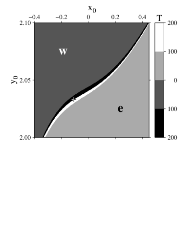
Figure 9: The saddle-trap map. Color modulates the time $T$ which $2.5\cdot 10^{5}$ particles with given initial positions ($x_{0},y_{0}$) need to reach the lines at $x=-1$ or $x=1$ escaping to the west (w) and to the east (e), respectively. The black and white diagonal curve is an image of a fragment of the stable manifold of the saddle trajectory. The cross is a position of a particle on that trajectory at the initial time moment. The integration time is $t=500$.

We have found that particles quit the ST along the unstable manifolds in accordance with specific laws. We distribute a large number of particles along the segment with $x_{0}=0$ and $y_{0}=[2.02;2.06]$, crossing the stable manifold $W_{s}$, and compute the time $T$ particles with given initial latitude positions $y_{0}$ need to quit the ST. More precisely, $T(y_{0})$ is a time moment when a particle with the initial position $y_{0}$ reaches the lines with $x=-1$ or $x=1$. The ‘‘experimental’’ points in Fig. 10 a fit the law $T_{\rm e}=(-85.81\pm 0.04)-(31.216\pm 0.007)\ln(y_{0s}-y_{0})$ for the particles which quit the trap moving to the east and the law $T_{\rm w}=(-60.61\pm 0.03)-(28.933\pm 0.006)\ln(y_{0}-y_{0s})$ for those particles which move to the west when quitting the trap, where $y_{0s}=2.0405755472$ is a crossing point of $W_{s}$ with the segment of initial positions.

Figure 10: (a) Time $T$ a particle with an initial latitude position $y_{0}$ needs to quit the saddle trap. (b) The number of short flights $n$ such a particle performs before quitting the saddle trap. The ranges of $y_{0}$ from which particles quit the trap moving to the west and east are denoted by ‘‘w’’ and ‘‘e’’, respectively.

The ST attracts particles and force them to rotate in its zone of influence performing short flights, the number of which $n$ depends on particle’s initial positions $y_{0}$. The $n(y_{0})$ is a steplike function (see Fig. 10 b) with the lengths of the steps decreasing in a geometric progression in the direction to the singular point, $l_{j}=l_{0}\,q^{-j}$, where $l_{j}$ is the length of the $j$-th step and $q\simeq 2.27$ for the western exits and $q\simeq 2.20$ for the eastern ones. The seeming deviation from this law in the range $y_{0}=[2.045;2.046]$ (see a small western segment between two larger ones in Fig. 10 b) is explained by crossing the initial line $y_{0}=[2.02;2.06]$ by the curve of zero zonal velocity $u$. To have the correct law for the western exits, it is necessary to add the two segments of that cut step. The asymmetry of the functions $T(y_{0})$ and $n(y_{0})$ is caused by the asymmetry of the flow.

5 Ballistic-islands traps

Besides the rotational islands with particles moving around the corresponding elliptic points in the same frame, we have found in Paper I ballistic islands situated both in the stochastic layer and in the peripheral currents. Regular ballistic modes [30] correspond to stable quasiperiodic inter-frame motion of particles. Only the ballistic islands in the stochastic layer are important for chaotic transport. Mapping positions of the regular ballistic trajectories at the moments of time $t_{n}=2\pi n/\omega$ $(n=1,2,\dots)$ onto the first frame, we obtain chains of ballistic islands both in the northern and southern stochastic layers, i. e., between the borders of the northern (southern) peripheral currents and of the corresponding vortex cores. A chain with three large ballistic islands is situated in those stochastic layers. The particles, belonging to these islands, move to the west, and their mean zonal velocity can be easily calculated to be $\left<u_{f}\right>=-2\pi/3T=-\omega/3\simeq-0.0845$. There are also chains of smaller-size ballistic islands along the very border with the peripheral currents.

We have demonstrated in Paper I a stickiness of chaotic trajectories to the borders of those three large ballistic islands (see Figs. 6 and 7 in Paper I). The Poincaré section with fragments of two chaotic trajectories in the northern stochastic layer is shown in Fig. 11 a. One particle performs a long flight sticking to the very border with the regular westward current, and another one moves to the west sticking to the very boundaries of three large ballistic islands. A magnification of a fragment of the border and tracks of a sticking trajectory around a smaller-size ballistic island are demonstrated in Fig. 11 b. Fig. 11 c demonstrates the effective size of the trap of the large ballistic islands with tracks of a sticking trajectory around them.

Figure 11: (a) Poincaré section of the northern stochastic layer where stickiness to the very border with the regular westward current and to three large ballistic islands are shown. Increased density of points along the border with the peripheral current is caused by the traps of the border ballistic islands one of which is shown in (b). (c) The trap of the large ballistic islands.

Figure 12: The distribution of a number of long westward flights with $T_{f}\geq 10^{3}$ over their mean zonal velocities $\left<u_{f}\right>$. The sharp peak corresponds to the trap connected with the very boundaries of the large ballistic islands, the left wing — to a number of traps of families of the border ballistic islands, and the right wing — to the trap situated around the large ballistic islands. Statistics for five tracers with the total number of long westward flights $N_{f}=5\cdot 10^{4}$ and the computation time $t=5\cdot 10^{8}$ for each tracer.

It is reasonable to suppose that the ballistic-islands traps (BIT) contribute, largely, to the statistics of long flights with $|x_{f}|\gg 2\pi$. All the ballistic particles, moving both to the west and to the east, can finish a flight and make a turn only in the strip shown in Fig. 1 c. The loci of the corresponding turning points have a complicated fractal-like structure. We consider further only long westward flights, taking place in the northern stochastic layer, because it is much wider than the stochastic layer between the regular central jet and the southern parts of the vortex cores where eastward flights take place.

To distinguish between contributions of the traps of different ballistic islands (and, maybe, other zones in the phase space) to the statistics of long flights, we compute for five long chaotic trajectories (up to $t=5\cdot 10^{8}$) the distribution of a number of westward flights with $T_{f}\geq 10^{3}$ over the mean zonal velocities $\left<u_{f}\right>=x_{f}/T_{f}$ of the particles performing such flights. The distribution in Fig. 12 has a prominent peak centered at the mean zonal velocity $\left<u_{f}\right>\simeq-0.0845$ which corresponds to a large number of long flights of those particles (and their trajectories) which stick to the very boundaries of the large ballistic islands (see Fig. 11 a) moving with the mean velocity $\left<u_{f}\right>\simeq-0.0845$. The flat left wing of the distribution $N(\left<u_{f}\right>)$ corresponds to the traps of smaller-size ballistic islands nearby the border with the peripheral current. There are different families of these islands (see one of them in Fig. 11 b) with their own values of the mean zonal velocity which are in the range $-0.092\lesssim\left<u_{f}\right>\lesssim-0.0845$. Stickiness to the boundaries of the border islands is weaker because they are smaller than the large islands and their contribution to the statistics of long flights is comparatively small.

The right wing of the distribution $N(\left<u_{f}\right>)$ with $-0.084\lesssim\left<u_{f}\right>\lesssim-0.075$ deserves further investigation. The value $\left<u_{f}\right>\simeq-0.075$ is a minimal value of the zonal velocity for long westward flights possible in the northern stochastic layer. Increasing the minimal duration of a flight from $T_{f}=10^{3}$ to $T_{f}=(2\div 5)\cdot 10^{3}$, we have found splitting of the broad distribution with $-0.084\lesssim\left<u_{f}\right>\lesssim-0.08$ into a number of small distinct peaks. Comparing trajectories with the values of $\left<u_{f}\right>$ corresponding to these peaks, we have found that all they move around the large ballistic islands. The particles with smaller values of $\left<u_{f}\right>$ used to penetrate further to the south from the islands more frequently than those with larger values of $\left<u_{f}\right>$ which prefer to spend more time in the northern part of the dynamical trap connected with those islands. Thus, we attribute the right wing of the distribution $N(\left<u_{f}\right>)$ to an effect of the trap situated around the large ballistic islands.

To estimate the contribution of different BITs to the statistics of long westward flights in Fig. 2 we have computed the PDFs $P(x_{f})$ and $P(T_{f})$ for particles performing westward flights with $x_{f}\geq 100$ and $T_{f}\geq 1000$ and with the mean zonal velocity $\left<u_{f}\right>$ to be chosen in three different ranges shown in Fig. 12: $-0.092\lesssim\left<u_{f}\right>\lesssim-0.085$ (particles sticking to the border islands) $-0.085<\left<u_{f}\right>\lesssim-0.084$ (particles sticking to the very boundary of three large islands), and $-0.084<\left<u_{f}\right>\lesssim-0.075$ (the trap of the three large islands). All the PDFs $P(x_{f})$ decay exponentially but with different values of the exponents equal to $\nu\simeq-0.005$ and $\nu\simeq-0.0018\div-0.0014$ for the traps of border and the large ballistic islands, respectively. The tail of the PDF $P(x_{f})$ for westward flights, shown in Fig. 2, decays exponentially with $\nu\simeq-0.0014$. Thus, the contribution of the large island’s BIT to the statistics of long westward flights is dominant. As to temporal PDFs $P(T_{f})$ for westward long flights, they are neither exponential nor power-law like with strong oscillations at the very tails. The slope for the border BITs is again smaller than for the large ballistic islands trap.

6 Conclusion

A meandering jet is a fundamental structure in oceanic and atmospheric flows. We described statistical properties of chaotic mixing and transport of passive particles in a kinematic model of a meandering jet flow in terms of dynamical traps in the phase (physical) space. The boundaries of rotational islands (including the vortex cores) in circulation zones are dynamical traps (RITs) contributing, mainly, to the statistics of short flights with $|x_{f}|<2\pi$. Characteristic times and spatial scales of the RITs have been shown to correlate with the PDFs for the lengths $x_{f}$ and durations $T_{f}$ of short flights. The stable manifolds of periodic saddle trajectories play a role of saddle traps (STs) with the specific values of the lengths and durations of short flights of the particles sticking to the saddle trajectories. The boundaries of ballistic islands in the stochastic layers (including those situated along the border with the peripheral current) are dynamical traps (BITs) contributing, mainly, to the statistics of very long flights with $|x_{f}|\gg 2\pi$.

Dynamical traps are robust structures in the phase space of dynamical systems in the sense that they present at practically all values of the corresponding control parameters. We never know exact values of the parameters in real flows, especially, in geophysical ones. We don’t know exactly the structure of the corresponding phase space, however, we know that typical features, like islands of regular motion, vortices, and jets, exist in real flows (see their images in some laboratory flows in Ref. [31]). In this paper we chose specific values of the control parameters for which specific PDFs have been computed and explained by the effect of those dynamical traps that exist under the chosen parameters. We have carried out computer experiments with different values of the control parameters and found that the phase space structure has been changed, of course, with changing the values of the parameters, but the corresponding RITs, STs, and BITs with specific temporal and spatial characteristics have been found to contribute to the corresponding statistics.

After finishing our work, we were acquainted with Ref. [32] where meridional chaotic transport, associated with a similar kinematic model of a meandering jet, has been studied by the method of lobe dynamics [33]. In difference from our study of zonal chaotic transport, a geometric structure of cross jet transport has been considered in Ref. [32] where values of the control parameters have been chosen to be sufficiently large to break up the central jet as a barrier to transport of particles across the jet. The mechanisms for particles to cross the jet have been described in terms of lobe dynamics and the mean time to cross the jet for particles entering the jet and the mean residence time for particles in the jet have been estimated in Ref. [32]. We have studied a more realistic situation (at least, for surface oceanic jet currents) when the jet is an absolute barrier to cross jet transport and we explained statistical properties of transport in terms of dynamical traps of saddle trajectories, rotational and ballistic islands. The method of lobe dynamics is hardly applicable for study zonal chaotic transport since it is practically impossible to trace out lobe evolution for a large number of frames.

References

- [1] S.V. Prants, M.V. Budyansky, M.Yu. Uleysky, and G.M. Zaslavsky, Chaos 16, 033117 (2006).
- [2] G.M. Zaslavsky, Phys. D. 168-169, 292 (2002).
- [3] H.A. Dijkstra, Nonlinear physical oceanography (Dordrecht, Kluwer, 2000).
- [4] S. Wiggins, Annu. Rev. Fluid Mech. 37, 295 (2005).
- [5] R.T. Pierrehumbert, Phys. Fluids 3, 1250 (1991).
- [6] M. Cencini, G. Lacorata, A. Vulpiani, and E. Zambianchi, J. Phys. Oceanogr. 29, 2578 (1999).
- [7] T.F. Shuckburgh and P.H. Haynes, Phys. Fluids 15, 3342 (2003).
- [8] V.I. Arnold, C. R. Hebd. Seances Acad. Sci. 261, 17 (1965).
- [9] M. Henon, C. R. Hebd. Seances Acad. Sci. 262, 312 (1966).
- [10] H. Lamb, Hydrodynamics (Dover, New York, 1945).
- [11] G.M. Zaslavsky, Phys. Rep. 371, 461 (2002).
- [12] G.M. Zaslavsky, Hamiltonian chaos and fractional dynamics (Oxford University Press, Oxford, 2005).
- [13] D. del-Castillo-Negrete and P.J. Morrison, Phys. Fluids A 5, 948 (1993).
- [14] R.M. Samelson, J. Phys. Oceanogr. 22, 431 (1992).
- [15] K. Ngan and T. Shepherd, J. Fluid Mech. 334, 315 (1997).
- [16] G.C. Yuan, L.J. Pratt, and C.K.R.T. Jones, Dyn. Atmos. Oceans. 35, 41 (2002).
- [17] M.V. Budyansky, M.Yu. Uleysky, and S.V. Prants, Nelineinaya Dinamika 2, 165 (2006) [in Russian].
- [18] J. Sommeria, S.D. Meyers, and H.L. Swinney, Nature (London) 337, 58 (1989).
- [19] R.P Behringer, S.D. Meyers, and H.L. Swinney, Phys. Fluids A 3, 1243 (1991).
- [20] T.H. Solomon, E.R. Weeks, and H.L. Swinney, Phys. Rev. Lett. 71, 3975 (1993).
- [21] T.H. Solomon, E.R. Weeks, and H.L. Swinney, Phys. D 76, 70 (1994).
- [22] A.S. Bower, J. Phys. Oceanogr. 21, 173 (1989).
- [23] A.S. Bower and H.T. Rossby, J. Phys. Oceanogr. 19, 1177 (1989).
- [24] B.V. Chirikov, Phys. Rep. 52, 263 (1979).
- [25] R.S. Mackay, J.D. Meiss, and I.C. Percival, Phys. D. 13, 55 (1984).
- [26] K.V. Koshel and S.V. Prants, Physics-Uspekhi 49, 1151 (2006) [Uspekhi Fizicheskikh Nauk 176, 1177 (2006)].
- [27] G.M. Zaslavsky, Chaos 5, 653 (1995).
- [28] G.M. Zaslavsky and B. Niyazov, Phys. Rep. 283, 73 (1997).
- [29] B.A. Petrovichev, A.V. Rogalsky, R.Z. Sagdeev, and G.M. Zaslavsky, Phys. Lett. A 150, 391 (1990).
- [30] V. Rom-Kedar and G. Zaslavsky, Chaos 9, 697 (1999).
- [31] J.M. Ottino, The kinematics of mixing: stretching, chaos, and transport (Cambridge University Press, Cambridge, 1989).
- [32] F. Raynal and S. Wiggins, Phys. D 223, 7 (2006).
- [33] W.S. Wiggins, Chaotic Transport in Dynamical System (Springer-Verlag, New York, 1992).