Correcting the apparent mutation rate acceleration at shorter time scales under a Jukes-Cantor model

Abstract.

At macroevolutionary time scales, and for a constant mutation rate, there is an expected linear relationship between time and the number of inferred neutral mutations (the “molecular clock”). However, at shorter time scales a number of recent studies have observed an apparent acceleration in the rate of molecular evolution.

We study this apparent acceleration under a Jukes-Cantor model applied to a randomly mating population, and show that, under the model, it arises as a consequence of ignoring short term effects due to existing diversity within the population. The acceleration can be accounted for by adding the correction term $h_{0}e^{-4\mu t/3}$ to the usual Jukes-Cantor formula $p(t)=\frac{3}{4}(1-e^{-4\mu t/3})$, where $h_{0}$ is the expected heterozygosity in the population at time $t=0$. The true mutation rate $\mu$ may then be recovered, even if $h_{0}$ is not known, by estimating $\mu$ and $h_{0}$ simultaneously using least squares.

Rate estimates made without the correction term (that is, incorrectly assuming the population to be homogeneous) will result in a divergent rate curve of the form $\mu_{\mathrm{div}}=\mu+C/t$, so that the mutation rate appears to approach infinity as the time scale approaches zero. While our quantitative results apply only to the Jukes-Cantor model, it is reasonable to suppose that the qualitative picture that emerges also applies to more complex models. Our study therefore demonstrates the importance of properly accounting for any ancestral diversity, as it may otherwise play a dominant role in rate overestimation.

1. Introduction

It is well-known since Kimura (1968; 1983) that over time scales of tens and hundreds of millions of years the longer term rate of molecular evolution, $k$, is expected to be virtually the same as the short term rate of neutral mutations $\mu$, that is, $k\approx\mu$. However, at shorter time scales a number of recent studies (for example García-Moreno (2004); Ho et al. (2005); Penny (2005); Millar et al. (2008); Henn et al. (2009); although there were some earlier indications (Fitch and Atchley, 1985)) have observed an apparent acceleration in the rate of molecular evolution. This has led to debate as to the underlying causes of the apparent acceleration, and raised important questions as to how long it persists and how to correct for it.

A number of factors that may contribute to this apparent rate acceleration have been proposed, and we refer the reader to Ho et al. (2011) for a recent review. One such factor is the effect of ancestral polymorphism (Peterson and Masel, 2009; Charlesworth, 2010). Indeed, it is clear that, if ancestral polymorphism is present and not properly accounted for, then an apparent rate acceleration will inevitably be seen. Consider a comparison between two sequences drawn from a population at time $t=0$ which is incorrectly assumed to be homogeneous. Any differences between the sequences due to polymorphism will appear to be mutations that have occurred in zero time, leading to an apparent infinite substitution rate at time zero. Moreover, on sufficiently short time scales the average difference due to polymorphism will dominate any changes due to substitution, and to first order the expected difference between sequences at times $0$ and $t$ will be given by $p(t)=C+\mu^{\prime}t$. (Here $\mu^{\prime}$ will differ slightly from the mutation rate $\mu$, as some mutations will act to decrease polymorphism.) Naively dividing by $t$ to recover $\mu$, under the assumption that the first order approximation is given by $p(t)=\mu t$, then gives an apparent divergent rate curve $\mu^{\prime}+C/t$, suggesting that unaccounted ancestral polymorphism will contribute a term of the form $C/t$ to rate estimates. This a priori estimate is in sharp contrast with the use of exponential decay curves of the form $k+\mu e^{-\lambda t}$ (for example, by Ho et al. (2005)) to fit estimated rates.

The effect of ancestral polymorphism on sequence divergence has been studied quantitatively by Peterson and Masel (2009), who calculate the expected divergence between two sequences as a function of time under the Moran model with selection. Their model provides a reasonable fit to data from Genner et al. (2007) and Henn et al. (2009), confirming that the observed rate acceleration is consistent with an underlying constant mutation rate. However, their model does not admit a simple closed form analytic expression, and this makes it difficult to correct for the apparent rate acceleration or quantify its duration.

The purpose of this paper is to quantify the effect of ancestral polymorphism under a Jukes-Cantor type model applied to a randomly mating population. This is a more restrictive setting than that considered by Peterson and Masel, but the benefit of working in this simpler setting is that we are able to obtain simple and explicit analytic expressions for quantities of interest. In particular, we show that, under the model, ancestral polymorphism contributes a term $h_{0}e^{-4\mu t/3}$ to the usual Jukes-Cantor formula $p(t)=\frac{3}{4}(1-e^{-4\mu t/3})$, where $h_{0}$ is the expected heterozygosity at time $t=0$, and confirm that comparisons between sequences made under the incorrect assumption $h_{0}=0$ lead to a divergent rate curve of the form $\mu_{\mathrm{div}}=\mu+C/t$. This has consequences at long time scales as well as short, as $C/t$ tends to zero comparatively slowly as $t$ tends to infinity (in particular, more slowly than any exponential decay), and so the effects of ancestral polymorphism may be relatively long lived. We show however that the true mutation rate $\mu$ may still be recovered from several observations even if the level of heterozygosity at time 0 is unknown, by estimating $h_{0}$ simultaneously with $\mu$ using least squares. We show further that our correction term also applies to other population structures (for example, island models) under an appropriate assumption on $h_{0}$.

These results show that ancestral polymorphism, where present and unaccounted for, will be a significant contributing factor to mutation rate overestimation, with the magnitude of the effect approaching infinity as the time scale shrinks to zero. Our principal finding then is that an apparent rate acceleration at short time scales is consistent with — and indeed to be expected under — a constant mutation rate, in the presence of ancestral polymorphism that is not properly taken into account. This finding is in agreement with that of Peterson and Masel (2009).

Ancestral polymorphism is just one of several processes that are thought to contribute to the apparent rate acceleration, and is unlikely to be the sole contributing factor. However, it is clearly vital that its effect be quantified and accounted for if we are to obtain meaningful and accurate rate estimates on short time scales, and fully resolve the question of the apparent acceleration.

2. The model, and our main result

We consider a population of $N$ individuals evolving under a random mating process, with discrete generations, where at each generation the allele of each individual is replaced with a copy of the allele from the previous generation, chosen uniformly at random (Wright, 1931). For simplicity we restrict our attention to haploid populations. We assume that alleles are $r$-state characters evolving under the $r$-state Jukes-Cantor model (Jukes and Cantor, 1969), with an instantaneous mutation rate of $\mu$ mutations per individual per generation per site. All mutations are assumed to be neutral. We orient time in the forwards direction, so that populations at times $t>0$ descend from the population at $t=0$. We refer to the population at time $0$ as the reference population, and the population at a given time $t>0$ of interest as the contemporary population.

Consider a pair of individuals chosen uniformly at random, one from each of the reference and contemporary populations, and let $P(t)$ be the probability that they have different character states at a fixed site. Suppose that the distribution of character states at that site in the reference population is given by $\pi=(\pi_{1},\ldots,\pi_{r})$. (Note that $\pi$ as used here is the distribution of states within the population at a given site, rather than the equilibrium distribution of the Jukes-Cantor model, which is the distribution of states across all sites within an individual.) Then

Theorem.

The probability that uniformly randomly chosen members of the reference and contemporary populations have different states at a given site is given by

(1) $$P(t)=h_{0}e^{-\frac{r}{r-1}\mu t}+\tfrac{r-1}{r}(1-e^{-\frac{r}{r-1}\mu t}),$$

where

$$h_{0}=P(0)=\sum_{i=1}^{r}\pi_{i}(1-\pi_{i})=\sum_{i}\sum_{j\neq i}\pi_{i}\pi_{j}$$

is the expected heterozygosity at $t=0$. In particular, for $r=4$ (as for nucleotides) we get

$$P(t)=h_{0}e^{-\frac{4}{3}\mu t}+\tfrac{3}{4}(1-e^{-\frac{4}{3}\mu t}).$$

The proof of the theorem is given in the Appendix. Note that the second term in equation (1) is the standard probability under the $r$-state Jukes-Cantor model that a net change takes place at the given site, when the contemporary sequence directly descends from the reference sequence — this second term is the usual form of the equation for longer time periods. Thus the theorem adds the correction term $h_{0}e^{-r\mu t/(r-1)}$ when the sequences being compared are not necessarily direct descendants. This accounts for the variation that is present in the reference population from past mutations that have not yet been either fixed or lost. The two expressions $P(t)$ and the Jukes-Cantor mutation probability are asymptotic, in the sense that

$$\frac{P(t)}{\tfrac{r-1}{r}(1-e^{-\frac{r}{r-1}\mu t})}=1+\frac{h_{0}e^{-\frac{r}{r-1}\mu t}}{\tfrac{r-1}{r}(1-e^{-\frac{r}{r-1}\mu t})}\rightarrow 1$$

as $t\to\infty$.

Note that the theorem requires that the population at the earlier time be used as the reference population. In particular, if populations at several different times are to be compared, then this should be done by comparing each population against the oldest population, to ensure that all pairwise comparisons made involve the same value of the initial heterozygosity $h_{0}$. This requirement may be relaxed if there is reason to believe that the heterozygosity $h$ is constant, or nearly so. In general, we expect $\pi$ (and hence $h$) to depend on $t$, but as $t\rightarrow\infty$ we also expect $\pi$ to approach an equilibrium distribution $\pi_{\infty}$, where the rate at which new mutations are introduced balances the rate at which mutations are fixed or lost by the mating process. If this equilibrium is assumed to have occurred then equation (1) may be written in the form

(2) $$P(t)=h_{\infty}e^{-\frac{r}{r-1}\mu t}+\tfrac{r-1}{r}(1-e^{-\frac{r}{r-1}\mu t}),$$

where $h_{\infty}$ is the expected heterozygosity at equilibrium. Under this assumption any two populations at times $t_{1}$ and $t_{2}$ may be compared, using $t=|t_{1}-t_{2}|$.

2.1. Recovering the mutation rate from observed data

We now demonstrate how the mutation rate $\mu$ may be estimated from observations of $P(t)$. If the expected heterozygosity is assumed to have reached equilibrium, then $h_{\infty}$ may be substituted for $h_{0}$ throughout.

Equation (1) may be rearranged to the form

(3) $$P(t)=\tfrac{r-1}{r}\left(1-(1-\tfrac{r}{r-1}h_{0})e^{-\frac{r}{r-1}\mu t}\right).$$

If $h_{0}$ is known then we may estimate $\mu$ as

(4) $$\mu=-\frac{r-1}{rt}\log\frac{1-\tfrac{r}{r-1}P(t)}{1-\tfrac{r}{r-1}h_{0}}.$$

On the other hand, if $h_{0}$ is not known then it will need to be estimated simultaneously with $\mu$. This may be done using a least squares fit to

$$\log\left(1-\tfrac{r}{r-1}P(t)\right)=\log(1-\tfrac{r}{r-1}h_{0})-\tfrac{r}{r-1}\mu t;$$

if the least squares line is $y=mt+b$ then we recover $\mu$ and $h_{0}$ as

$$\mu =-\tfrac{r-1}{r}m, h_{0} =\tfrac{r-1}{r}(1-e^{b}).$$

2.2. The divergent rate curve

A divergent rate curve arises when we either omit or use an incorrect value for $h_{0}$ to estimate $\mu$. In particular, if we ignore the existing diversity and thus use $h_{0}=0$ we get the estimate

(5) $$\mu_{\mathrm{div}} =-\frac{(r-1)\log(1-\tfrac{r}{r-1}P(t))}{rt}$$

$$=\mu-\frac{(r-1)\log\left(1-\tfrac{r}{r-1}h_{0}\right)}{rt},$$

which adds the divergent term $\frac{(1-r)\log\left(1-\tfrac{r}{r-1}h_{0}\right)}{rt}$ to the estimate above. Thus, if the variation present within the reference population is ignored we obtain a divergent rate curve of the form $\mu_{\mathrm{div}}=\mu+C/t$, where $C=\frac{1-r}{r}\log\left(1-\tfrac{r}{r-1}h_{0}\right)$ is a positive constant independent of $t$. This rate estimate tends to infinity as $t\to 0$, and thus becomes increasingly inaccurate on shorter and shorter times scales.

3. Results of simulations

Figure 1A shows results of simulations over microevolutionary time scales, and exhibits the phenomena described above. Most importantly, if we do not correct for existing genetic diversity there is the apparent acceleration at shorter times, even though the basic neutral mutation rate $\mu$ is kept constant. This first main point then is that the apparent increase in “rate” (the divergent rate curve) is obtained at shorter periods. However, it is then important that, using equation (4) and the value of $h_{0}$, the value of $\mu$ can still be estimated accurately at these shorter intervals. This is certainly as expected; it has always been assumed that the mutation rate $\mu$ was basically constant, that it was independent of time. Thus the conclusion from Figure 1A is that by explicitly considering genetic variability in the ancestral (reference) population — either by using an a priori estimate of it (blue curve), or by estimating it simultaneously using least squares (dashed black line) — it is possible to recover the mutation rate $\mu$. In practice, it may be that knowledge of $\mu$ (from longer term studies) may also be important in understanding population structure and its change over time.

3.1. The simulations

The simulations were run using the statistical package R (2011). Each simulation begins with a haploid population containing 70 individuals having allele A and 30 individuals having allele B, giving a true $h_{0}$ of 0.42. There are four allele types in total, and mutations from any given allele to any of the other three take place at equal rates, as in the Jukes-Cantor model for DNA substitutions. This population is then evolved for 1000 generations. In each generation, reproduction is simulated according to the Wright-Fisher process, whereby each of the 100 individuals making up the new population is chosen randomly with replacement from the previous generation; each of these new individuals is then subjected to mutation at the rate of $\mu=0.001$ mutations per individual per generation. For the final step in each generation, a pair of individuals — one from the current population and one from the initial population — is picked randomly and compared; if they have different alleles, a counter for that generation is increased by 1. The entire simulation was repeated 2000 times, with counters accumulating across runs: consequently the final counter value for generation $i$, after dividing by 2000, is an estimate of the probability that an individual picked randomly from the initial population differs from an individual picked randomly from generation $i$. These relative frequencies are used to estimate the mutation rate parameter $\mu$ in several different ways, as we now describe.

3.2. Estimating $\mu$

Three different approaches to estimating $\mu$ are shown in Figure 1A. The dashed pink curve shows the result of estimating $\mu$ while incorrectly assuming $h_{0}=0$ (the assumption made by most previous studies); the solid blue curve shows the result of estimating $\mu$ assuming $h_{0}$ to be its true value, 0.42. The difference is plain, particularly at early times when the probability of observing a difference is dominated by the heterozygosity of the initial population. To demonstrate the limited accuracy achievable using the incorrect assumption that $h_{0}=0$, the $\mu$ curve that would be estimated from an infinite number of observations (instead of 2000) is shown as a dashed green line — it is scarcely better, indicating that sampling error is not the problem. The fact that the pink curve tracks the dashed green curve also indicates that, as expected, the simulation fits our theoretical divergent curve $\mu_{\mathrm{div}}$ of equation (5). Note that the erratic behaviour of the blue curve near 0 is due to numerical instability, as the calculations there involve logs and ratios of numbers close to zero.

Both of the above estimation procedures can estimate $\mu$ using a probability estimate from a single time point, but assume $h_{0}$ to be known a priori. Where this is not the case, $h_{0}$ can be estimated simultaneously with $\mu$ using least squares, which requires probability estimates from multiple time points. The result of estimating a single value for $\mu$ using all 1001 time points is shown as a horizontal dashed black line in Figure 1A.

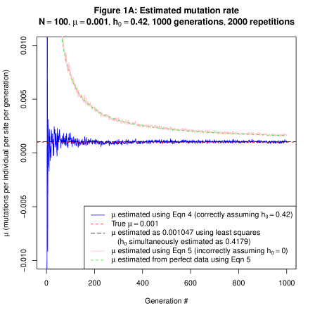
Figure 1. Estimated mutation rates against time for three different population structures. (1A): A single population initially containing 70 individuals having allele A and 30 individuals having allele B; (1B): A 2-island model, both of whose subpopulations are initially the same as for (1A), with 1% migration per generation from island 1 to island 2, and 10% migration per generation in the reverse direction; (1C): A 2-island model, whose first subpopulation is the same as for (1A), and whose second subpopulation contains 25 individuals of each of the four states. The graphs show the results of simulations of four state data. Dashed red line: the value of the mutation rate $\mu$ used. Blue curve: $\mu$ estimated at each time point from simulated data transformed using equation (4) and the correct value for the ancestral heterozygosity $h_{0}$. Pink curve: simulated data transformed using the incorrect transform (equation (5)) to estimate $\mu$, giving a divergent rate curve. Dashed green curve (1A, 1B): theoretical divergent rate curve, obtained by transforming perfect data (equation (1)) according to equation (5). This assumes an incorrect value of $h_{0}$= 0. Dashed black line: the least squares estimate of $\mu$ from the simulated data. This uses no knowledge of $h_{0}$ or $\mu$ (unlike the blue curve). Note that the blue curve behaves poorly near 0, where the calculations are numerically unstable as they involve logs and ratios of numbers close to zero.

3.3. Other population structures

Our corrected formula extends to cases where the population consists of multiple subpopulations that interact via arbitrary migration rates, provided that the initial distribution of states is the same for each subpopulation. Figure 1B shows the accurate recovery of $\mu$ and $h_{0}$ for a simulated population consisting of two islands, each containing 70 individuals having allele A and 30 individuals having allele B, that mix sporadically and asymmetrically: in each generation, the probability that an individual in subpopulation 1 comes from subpopulation 2 is just 1%, while the probability that an individual in subpopulation 2 comes from subpopulation 1 is 10%. Adding this limited kind of population structure does not alter the fact that the probability distribution of states for the ancestor of an individual chosen randomly at time $t$ remains equal to that for an individual chosen randomly from the initial population, so the probability $p_{\mathrm{diff}}$ that the ancestral and reference states differ is still given by $h_{0}$.

If the initial state distributions differ across subpopulations, then the probability that the ancestor of a randomly-chosen contemporary individual has a particular state is no longer constant, so $h_{0}$ in equation (1) must be replaced with a function of time, $p_{\mathrm{diff}}(t)$. Figure 1C shows results from a simulation of one such scenario. There are two islands, each containing 100 individuals: the first contains 70 individuals having allele A and 30 individuals having allele B, the second contains 25 individuals with each of the four alleles. Migration rates are as for Figure 1B. The blue curve, which shows an attempt to estimate $\mu$ using equation (4) and assuming that $h_{0}=0.6675$ (the probability that two individuals chosen randomly from the initial population have different states), produces a divergent rate curve because this more general population structure violates the assumption that $p_{\mathrm{diff}}$ is constant and equal to $h_{0}$.

Despite the fact that $p_{\mathrm{diff}}$ is nonconstant when the subpopulations have different initial state distributions, our approach is still useful here. Under reasonable conditions on migration probabilities, the probability that the ancestor of a randomly-chosen individual has a given state converges towards an equilibrium value as $t\to\infty$, and so $p_{\mathrm{diff}}$ will approach an equilibrium value also. In particular, when estimating $\mu$ and $h_{0}$ simultaneously via least squares, only the estimate of $h_{0}$ is affected by different initial state distributions across subpopulations: as expected, the dashed black line depicting the least squares estimate of $\mu$ in Figure 1C is close to the true value of $\mu$. Since $\mu$ is usually the parameter of interest, this means that our model can still be used for inference with these more general population structures. Note that any edge-weighted graph describing mating probabilities within a population can be represented as a multi-island model in which each island contains a single individual.

4. Conclusions

The Jukes-Cantor model is one of the oldest and simplest substitution models, and the benefit of studying ancestral polymorphism in this simple setting is that we are able to obtain explicit analytic expressions for quantities of interest, including the expected divergence between two sequences, and the uncorrected rate curve $\mu_{\mathrm{div}}$. Moreover, many more complex and realistic models include the Jukes-Cantor model as a special case, so while our precise quantitative findings are only supported under the limited model considered here, there are clear qualitative implications for these more general models.

Given the rapid advance in DNA sequencing technology we expect a large increase in sequences that have diverged in recent, intermediate and longer times. It is therefore essential to be able to generalise results to a full range of divergence times — it is no longer appropriate to consider separately shorter term microevolutionary and longer term macroevolutionary studies. Our results show that a significant contributing factor to the apparent acceleration at shorter times is the pre-existing diversity within a population, and this can be estimated for a wide range of population sizes and structures (Charlesworth and Charlesworth, 2010). By considering the expected diversity in a population we show how the real rate of neutral mutation can be estimated at shorter times, using either an appropriate estimate of genetic diversity or data from multiple time points. As the timescales of traditional phylogenetics and population genetics draw closer together, we anticipate seeing an increasing emphasis on the careful handling of genetic diversity in phylogenetic analyses; the work presented here can provide a starting point for the exploration of more general models involving more complex substitution processes, time-varying population sizes, and other effects.

Appendix A Proof of the main result

The individual chosen from the contemporary population descends from a unique member of the reference population, and this ancestor is equally likely to be any member of the reference population. We may therefore calculate the probability that the contemporary and reference states differ by considering two cases: the ancestral state agrees with the reference state, but evolves to disagree; and the ancestral state disagrees with the reference state, and evolves so as to remain in disagreement at time $t$.

Under the $r$-state Jukes-Cantor model the probability that there is a net transition from state $i$ to state $j\neq i$ in time $t$ is given by

$$p(t)=\tfrac{1}{r}(1-e^{-\frac{r}{r-1}\mu t}).$$

The probability that the ancestral state agrees with the reference state but evolves to disagree is therefore given by

(6) $$\sum_{i}\pi_{i}^{2}(r-1)p(t)=(r-1)p(t)\sum_{i}\pi_{i}^{2},$$

while the probability that both the ancestral and contemporary states differ from the reference is given by

(7) $$\sum_{i}\sum_{j\neq i}\pi_{i}\pi_{j}(1-p(t)) =(1-p(t))h_{0}.$$

Observe that

$$1=\left(\sum_{i}\pi_{i}\right)^{2}=\sum_{i}\pi_{i}^{2}+\sum_{i}\sum_{j\neq i}\pi_{i}\pi_{j}=h_{0}+\sum_{i}\pi_{i}^{2},$$

so $\sum_{i}\pi_{i}^{2}=1-h_{0}$. Hence summing equations (6) and (7) we get

$$P(t) =(1-h_{0})(r-1)p(t)+h_{0}\left(1-p(t)\right)$$

$$=(r-1)p(t)+h_{0}(1-p(t)-(r-1)p(t))$$

$$=(r-1)p(t)+h_{0}(1-rp(t))$$

$$=\frac{r-1}{r}(1-e^{-\frac{r}{r-1}\mu t})+h_{0}e^{-\frac{r}{r-1}\mu t},$$

as claimed.

References

- Charlesworth and Charlesworth (2010) B. Charlesworth and D. Charlesworth. Elements of evolutionary genetics. Roberts and Co., Greenwood Village, Colo., 2010.
- Charlesworth (2010) D. Charlesworth. Don’t forget the ancestral polymorphisms. Heredity, 105:509–510, 2010.
- Fitch and Atchley (1985) W. M. Fitch and W. R. Atchley. Evolution in inbred strains of mice appears rapid. Science, 228(4704):1169–1175, 1985.
- García-Moreno (2004) J. García-Moreno. Is there a universal mtDNA clock for birds? Journal of Avian Biology, 35(6):465–468, 2004.
- Genner et al. (2007) Martin J. Genner, Ole Seehausen, David H. Lunt, Domino A. Joyce, Paul W. Shaw, Gary R. Carvalho, and George F. Turner. Age of cichlids: New dates for ancient lake fish radiations. Mol. Biol. Evol., 24(5):1269–1282, 2007.
- Henn et al. (2009) B. M. Henn, C. R. Gignoux, M. W. Feldman, and J. L. Mountain. Characterizing the time dependency of human mitochondrial DNA mutation rate estimates. Molecular Biology and Evolution, 26(1):217–230, 2009.
- Ho et al. (2005) S. Y. W. Ho, M. J. Phillips, A. Cooper, and A. J. Drummond. Time dependency of molecular rate estimates and systematic overestimation of recent divergence times. Molecular Biology and Evolution, 22(7):1561–1568, 2005.
- Ho et al. (2011) S. Y. W. Ho, R. Lanfear, L. Bromham, M. J. Phillips, J. Soubrier, A. G. Rodrigo, and A. Cooper. Time-dependent rates of molecular evolution. Molecular Ecology, 20(15):3087–3101, 2011.
- Jukes and Cantor (1969) T. H. Jukes and C. R. Cantor. Evolution of protein molecules. In H. N. Munro and J. B. Allison, editors, Mammalian protein metabolism, pages 21–123. Academic Press, New York, 1969.
- Kimura (1968) M. Kimura. Evolutionary rate at the molecular level. Nature, 217(5129):624–626, 1968.
- Kimura (1983) M. Kimura. The neutral theory of molecular evolution. Cambridge University Press, 1983.
- Millar et al. (2008) C. D. Millar, A. Dodd, J. Anderson, G. C. Gibb, P. A. Ritchie, C. Baroni, M. D. Woodhams, M. D. Hendy, and D. M. Lambert. Mutation and evolutionary rates in adélie penguins from the antarctic. PLoS Genetics, 4(10), 2008.
- Penny (2005) D. Penny. Evolutionary biology: Relativity for molecular clocks. Nature, 436(7048):183–184, 2005.
- Peterson and Masel (2009) G. I. Peterson and J. Masel. Quantitative prediction of molecular clock and at short timescales. Molecular Biology and Evolution, 26(11):2595–2603, 2009.
- R Development Core Team (2011) R Development Core Team. R: A Language and Environment for Statistical Computing. R Foundation for Statistical Computing, Vienna, Austria, 2011.
- Wright (1931) S. Wright. Evolution in Mendelian populations. Genetics, 16(2):97–159, 1931.