Evaluating Network Models: A Likelihood Analysis

Abstract

Many models are put forward to mimic the evolution of real networked systems. A well-accepted way to judge the validity is to compare the modeling results with real networks subject to several structural features. Even for a specific real network, we cannot fairly evaluate the goodness of different models since there are too many structural features while there is no criterion to select and assign weights on them. Motivated by the studies on link prediction algorithms, we propose a unified method to evaluate the network models via the comparison of the likelihoods of the currently observed network driven by different models, with an assumption that the higher the likelihood is, the better the model is. We test our method on the real Internet at the Autonomous System (AS) level, and the results suggest that the Generalized Linear Preferential (GLP) model outperforms the Tel Aviv Network Generator (Tang), while both two models are better than the Barabási-Albert (BA) and Erdös-Rényi (ER) models. Our method can be further applied in determining the optimal values of parameters that correspond to the maximal likelihood. Experiment indicates that the parameters obtained by our method can better capture the characters of newly-added nodes and links in the AS-level Internet than the original methods in the literature.

I Introduction

Recent years have witnessed a fast development of complex networks Albert_rmp_2002 ; Dorogovtsev_aip_2002 ; Newman_siam_2003 ; Barabasi_science_2009 . A network is a set of items that are called vertices with connections between them, which are named as edges. Many natural and man-made systems can be described as networks. Such paragons cannot be numbered that biological networks including protein-protein interaction networks HJ_nature_2001 and metabolic network HJ_nature_2000 ; social networks such as movie actor collaboration He_physicaa_2006 and scientific collaboration networks Newman_pnas_2001 ; technological networks like power grids Watts_nature_1998 , WWW Albert_nature_1999 and the Internet at the Autonomous System (AS) level Bu_infocom_2002 ; Zhou_2003 ; Park_infocom_2004 ; Zhou_pre_2004 ; Bar_lncs_2004 ; Zhang_njp_2008 . A major endeavor in academics is to discover the common properties shared by many real networks and the specific features owned by a certain type of networks. A great number of measurements to reveal the structural features of networks are applied Costa_ap_2007 . The degree distribution Clauset_siam_2009 , as one of the most important global measurements, has attracted increasing attention since the awareness of the scale-freeness Barabasi_science_1999 . Clustering coefficient is a local measurement that characterizes the loop structure of order three. Another significant measurement is the average distance. A network is considered to be small-world if it has large clustering coefficient but short average distance Watts_nature_1998 . Except for the properties mentioned above, there are many other measurements such as degree-degree correlation Callaway_pre_2001 , betweenness centrality Freeman_sociometry_1977 and so forth. Moreover, some statistical measurements borrowed from physics such as entropy Shannon_BSTJ_1948 , and novel metrics such as modularity Newman_pnas_2006 also play important roles in characterizing networks.

Not only the statistical features but also the dynamical evolution of networks the current research interest has focused on. A mess of models have been proposed to reveal the origins of the impressive statistical features of complex networks. There are also many evolving models developed for some certain type of networks such as the Internet at the AS level Bu_infocom_2002 ; Zhou_2003 ; Park_infocom_2004 ; Zhou_pre_2004 ; Bar_lncs_2004 ; Zhang_njp_2008 , the social networks Viscek_physciaa_2002 ; Arenas_pre_2004 ; Kumar_2010 ; Huang_wsdm_2008 ; Albert_prl_2000 ; Dorogovtsev_pre_2000 and so forth. However the prosperous development of measurements sets a barrier for evaluating different evolving models. The traditional idea is that: if the network generated by a model resembles the target network in terms of some statistical features usually selected by the authors themselves, the model is claimed as a proper description of the real evolution. But this methodology seems to be puzzling. First, unselected statistical properties are entirely ignored so no one knows whether the model is sufficient to describe them as well. Secondly, the authors tend to select the metrics that support their models. Therefore, it is impossible to give a fair remark that which model is better. Thirdly, it is difficult to quantify the extent to which the models resemble the real evolving mechanisms.

Inspired by the link prediction approaches and likelihood analysis, we propose a method that tries to fairly and objectively evaluate different models. Link prediction aims at estimating the likelihood of non-existing edges in a network and try to dig out the missing edges Lv_physicaa_2011 . The evolution of networks involves two processes - one is the addition or deletion of nodes and another one is the changing of edges between nodes Albert_prl_2000 . In principle the rules of the additions of edges of a model can be considered as a kind of link prediction algorithm and here lies the bridge between link prediction and the mechanism of evolving models.

The present paper is organized as follows. We will give a general description of our method in Section II. Section III introduces the data and explains how to use our method to evaluate evolving models in details with the AS-level Internet being an example network. The results obtained by our method are shown in Section IV. We draw the conclusion and give some discussion in the last section.

II Method

In this section, we will give a general description about our method to evaluate evolving models. It is believed that an evolving model is a description of the evolving process of a network in reality. An evolving model describes the evolving mechanism of a real network or a class of networks. Given two snaps of one network at time $t_{1}$ and $t_{2}$ ($t_{1}<t_{2}$), as well as an evolving model, we can in principle calculate the likelihood that the network starting from the configuration at time $t_{1}$ will evolves to the configuration at $t_{2}$ under the rules of the given model. We say a model is better than another one if the likelihood of the former model is greater than that of the latter one. However, how to calculate such likelihood is still a big challenge. Inspired by the like prediction algorithms, we can calculate the likelihood of the addition of an edge according to a given evolving model Lv_physicaa_2011 . In a short duration of time, each edge’s generation can be thought as independent to others and the sequence of generations can be ignored. Thus the likelihood mentioned above is the product of the newly generated edges’ likelihoods.

Denote by $G$ the network and $E_{t}$ the set of edges at time step $t$. The new edges generated at the current time step is $E_{new}=E_{t+1}\backslash E_{t}$. The probability that node $i$ is selected as one end of the newly generated edge is

$$\Pi_{i}=f(G,\vec{a}),$$ (1)

where $\vec{a}$ is the set of parameters applied by the model. Then the likelihood of a new monitored edge $(i,j)$ is

$$P_{(i,j)}=\Pi_{i}\times\Pi_{j}.$$ (2)

Eq. (2) is applicable only when $i$ and $j$ are both old nodes. If $i$ or $j$ is newly generated, we set $\Pi_{i}=1$ or $\Pi_{j}=1$. In order to make comparison between different models, $P(i,j)$ is normalized by $1/\sum_{(a,b)\in E^{N}}{p(a,b)}$, where $E^{N}$ is the set of nonexisting edges($(i,j)\in E^{N}$). Given different parameters $\vec{a}$, the values of $P(i,j)$ may be different, resulting in different likelihoods of the target network. The parameters corresponding to the maximum likelihood are intuitively considered to be the optimal set of parameters for the evaluated model. In a word, a network’s likelihood can be calculated if the evolution data and the corresponding model are given. And if there are several candidate models, our method could judge them by comparing the corresponding likelihoods: the model giving higher likelihood according to the target network is more favored.

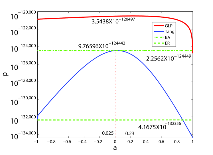
Figure 1: Likelihoods for different models and different parameters.

.

III Experimental Analysis

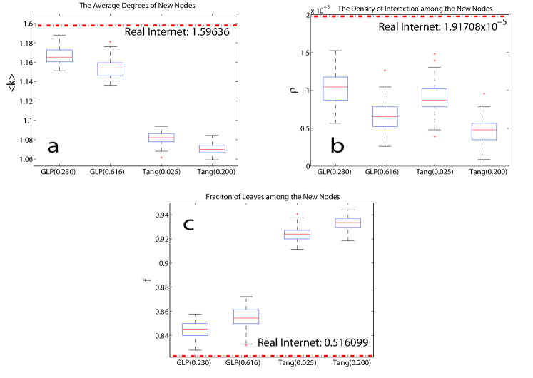
Figure 2: (a) The average degree of the newly generated nodes; (b) The density among the newly generated nodes; (c) The fraction of leaves in the newly generated nodes. Dash line in each plot represents the values for the real Internet. The structural features corresponding to the networks obtained by our suggesting parameters are closer to the reality. For each model with each parameter, we generate $100$ networks and use the so-called box-and-whisker plot boxplot to display the results, where the horizontal lines from top to bottom respectively stand for the maximum, the upper quartile, the median, the lower quartile and the minimum of a set of data.

In this paper we focus on the models of the AS-level Internet. Two popular models - Generalized Linear Preferential model (GLP) Bu_infocom_2002 and Tel Aviv Network Generator (Tang) Bar_lncs_2004 - will be evaluated by our method. The well-known Barabási-Albert (BA) Barabasi_science_1999 and Erdös-Rényi (ER) Erdos_1960 ; Bollobas_1985 models are also analyzed as two benchmarks.

The data sets we utilize here are collected by the Routeviews Project RP_website . We use the data of Jun. 2006 and Dec. 2006. Some nodes and edges in Jun. 2006 disappear in the record of Dec. 2006. Although an autonomous system might be canceled, rarely does it happen during a short time span. Therefore we assume that the nodes and edges in Jun. 2006 will not disappear in Dec. 2006. That is to say that the network configuration in Jun. 2006 is a subgraph of that in Dec. 2006. We merge the network of Jun. 2006 into that of Dec. 2006 to make a set substraction between the two sets to obtain the newly generated edges and nodes. The basic information of the processed data set of Dec. 2006 and two original data sets is shown in Table 1.

Table 1: The number of nodes and edges of the three data sets: two real data sets and one data set that is processed as we describe in the paper.

Time	# Nodes	# Edges
2006.06	22960	49545
2006.12	24403	52826
2006.12 (processed)	25103	59268

Now we will describe how to calculate the likelihood of each newly-generated edge in terms of the four models. (i) GLP model - This model starts from a few nodes. At each time step, with the probability $1-p$, one new node is added and $m$ edges are generated between the new node and $m$ old ones and with the probability $p$, $m$ edges are generated among the existing nodes. The ends of new edges are selected following the rule of generalized linear preferential attachment as

$$\Pi_{i}=\frac{k_{i}-\beta}{\sum_{j}{(k_{j}-\beta)}},$$ (3)

in which $\beta\in(-\infty,1)$. In our method if the end $i$ of a new edge is selected among the existing nodes, then $\Pi_{i}$ is calculated by the Eq. (3). Otherwise, if the end $i$ itself is a new node, $\Pi_{i}$ is $1$. So the likelihood of a new edge connecting two existing nodes $a$ and $b$ is

$$P_{(a,b)}=\frac{k_{a}-\beta}{\sum_{j}{(k_{j}-\beta)}}\frac{k_{b}-\beta}{\sum_{j}{(k_{j}-\beta)}}.$$ (4)

The likelihood of an edge generated between a new node $b$ and an existing node $a$ is

$$P_{(a,b)}=\frac{k_{a}-\beta}{\sum_{j}{(k_{j}-\beta)}}.$$ (5)

When a new edge connects two new nodes $a$ and $b$, its likelihood is

$$P_{(a,b)}=1.$$ (6)

(ii) Tang model - This model applies a super linear preferential mechanism, say

$$\Pi_{i}=\frac{k^{1+\epsilon}_{i}}{\sum_{j}{k^{1+\epsilon}_{j}}}.$$ (7)

This model also starts with a few nodes and at each time step a new node is generated with one edge connecting to one of the existing nodes that is selected with the probability described in Eq. (7). The remaining $m-1$ edges are added between the existing nodes. For these $m-1$ nodes, one end is selected according to Eq. (7), while the other one is selected randomly. Hence the likelihood of a new edge between existing nodes is

$$P_{(a,b)}=\frac{1}{N}\sqrt{\frac{k_{a}^{1+\epsilon}}{\sum_{j}{k_{j}^{1+\epsilon}}}\frac{k_{b}^{1+\epsilon}}{\sum_{j}{k_{j}^{1+\epsilon}}}},$$ (8)

where $N$ is the current size of the monitored network. Eq. (8) takes a geometric mean due to the fact that either $a$ or $b$ could be the one selected randomly. The cases involving new nodes are managed in the same way as that for the GLP model. (iii) BA model - The BA model also starts from a small graph and at each time step a new node associated with $m$ edges is added. The probability that the existing node $i$ is selected is

$$\Pi_{i}=\frac{k_{i}}{\sum_{j}{k_{j}}}.$$ (9)

Note that the original BA model cannot deal with the situation where edges are generated between two existing nodes. We thus generalize the BA model as if one edge is generated between two existing nodes, one node is selected preferentially following the Eq. (9) and another one is selected randomly. Therefore the likelihood of an edge between two existing nodes $a$ and $b$ is calculated as

$$P_{(a,b)}=\frac{1}{N}\sqrt{\frac{k_{a}}{\sum_{j}{k_{j}}}\frac{k_{b}}{\sum_{j}{k_{j}}}}.$$ (10)

The likelihood of an edge connecting a new node $b$ and an old one $a$ is

$$P_{(a,b)}=\frac{k_{a}}{\sum_{j}{k_{j}}}.$$ (11)

The likelihood of a new edge generated between two new nodes is $1$ as discussed above. (iv) ER model - The mechanism of this model is that when one edge is generated, both its ends are selected in a random fashion. The likelihood of one edge $(a,b)$ between two old nodes is

$$P_{(a,b)}=\frac{1}{N^{2}}.$$ (12)

The calculation of other two types of edges is similar to that of GLP. Note that BA is a special case equivalent to the GLP model when $\beta=0$. It is also obvious that the ER model is a special case of the Tang model when $\epsilon=0$.

Table 2: Maximum likelihoods and the corresponding parameters for the four models.

Model	Maximum Likelihood	Optimum parameters
GLP	$3.54\times 10^{-120497}$	$0.230$
Tang	$9.77\times 10^{-124442}$	$0.025$
ER	$4.17\times 10^{-132356}$	N/A
BA	$2.26\times 10^{-124449}$	N/A

The likelihoods of the four evolving models with different parameters are shown in Figure 1. The maximum likelihoods as well as the corresponding parameters are listed in Table 2. The maximum likelihoods of both specific Internet models (GLP and Tang) are greater than those of the BA model and the ER model. Notice that the BA and ER model are parameter-free and thus represented by two straight lines in Figure 1. Our results suggest that subject to the mimicking of the AS-level Internet evolution, the GLP model is better than the Tang model, and the Tang model is better than the BA model, of course, the ER model performs the worst. A puzzling point is that the optimal parameters corresponding to the maximum likelihoods are far from the ones suggested in the original literature Bu_infocom_2002 ; Bar_lncs_2004 . We next devise an experiment to demonstrate that the parameters obtained by our method are more advantageous than the original ones.

Traditionally, an evolving model starts from a small network with a few nodes. In this experiment, we respectively use the GLP and Tang models to drive the network evolution starting from the configuration of Jun. 2006, ending with the same size of the configuration of Dec. 2006. According to the Refs. Bu_infocom_2002 ; Bar_lncs_2004 and the data, $\beta=0.616,m=1.13,p=0.5214$ and $\epsilon=0.2$. Then we analyze some statistical features of the newly generated part including the average degree, the density of interaction and the fraction of leaves. We find that the performance of the GLP model is better than the Tang model with the same kind of parameters in the three cases, demonstrating that our evaluating method is reasonable. For both the two models, the statistical features obtained by the optimum parameters suggested by us resemble the real data better than those obtained by using the original parameters. The comparisons are shown in Figure 2.

IV Conclusion and Discussion

Thousands of network models are put forward in recent ten years. Some of them aim at uncovering mechanisms that underlie general topological properties like scale-free nature and small-world phenomenon, others are proposed to reproduce structural features of specific networks, such as the Internet, the World Wide Web, co-authorship networks, food webs, protein-protein interacting networks, metabolic networks, and so on. Besides the prosperity, we are worrying that there is no unified method to evaluate the performance of different models, even if the target network is given beforehand.

Instead of considering many structural metrics, this paper reports an evaluating method based on likelihood analysis, with an assumption that a better model will assign a higher likelihood to the observed structure. We have tested our method on the real Internet at the AS level, and the results suggest that the GLP model outperforms the Tang model, and both models are better than the BA and ER models. This method can be further applied in determining the optimal parameters of network models, and the experiment indicates that the parameters obtained by our method can better capture the structural characters of newly-added nodes and links.

The main contributions of this work are twofold. In the methodology aspect, we provide a starting point towards a unified way to evaluate network models. In the perspective aspect, we believe for majority of real evolutionary networks, the driven factors and the parameters will vary in time. For example, recent empirical analysis suggests that before and after the year 2004, the Internet at the AS level grows with different mechanisms Zhang_njp_2008 . To find out a single mechanisms that drives a network from a little baby to a giant may be an infeasible task. In fact, in different stages, a network could grow in different ways, or in a hybrid matter with changing weight distribution on several mechanisms. Once, the research focus has shifted from analyzing static models to evolutionary models. In the near future, it may shift from the evolutionary models to the evolving of the evolutionary models themselves. In principle, the current method could capture the tracks of not only the network evolution, but also the mechanism evolution. Hopefully this work could provide some insights into the studies on network modeling.

- (1) R. Albert and A.-L. Barabási, Rev. Mod. Phys. 74, 47 (2002).
- (2) S. N. Dorogovtsev and J. F. F. Mendes, Adv. Phys. 51, 1079 (2002).
- (3) M. E. J. Newman, SIAM Rev. 45, 167 (2003).
- (4) A.-L. Barabási, Science 325, 412 (2009).
- (5) H. Jeong, S. P. Mason, A.-L. Barabási, and Z. N. Oltvai, Nature (London) 411, 41 (2001).
- (6) H. Jeong, B. Tombor, R. Albert, Z. N. Oltvai, and A.-L. Barabási, Nature (London) 407, 651 (2001).
- (7) P.-P. Zhang, K. Chen, Y. He, T. Zhou, B.-B. Su, Y. Jin, H. Chang, Y.-P. Zhou, L.-C. Sun, B.-H. Wang, and D.-R. He, Physica A 360, 599 (2006).
- (8) M. E. J. Newman, Proc. Natl. Acad. Sci. U.S.A. 98, 404 (2001).
- (9) D. J. Watts and S. H. Strogatz, Nature (London) 393, 440 (1998).
- (10) R. Albert, H. Jeong, and A.-L. Barabási, Nature (London) 401, 130 (1999).
- (11) T. Bu and D. Towsley, in Proc. of IEEE INFOCOM 2002, p. 638.
- (12) S. Zhou and R. J. Mondragon, in Proc. of the 18th International Teletraffic Congress, p. 121.
- (13) S. T. Park, D. M. Pennock, and C. L. Giles, in Proc. of IEEE INFOCOM 2002, p. 1616.
- (14) S. Zhou and R. J. Mondragon, Phys. Rev. E 70, 066108 (2004).
- (15) S. Bar, M. Gonen, and A. Wool, Lect. Notes Comput. Sci. 3015, 53 (2004).
- (16) G.-Q. Zhang, G.-Q. Zhang, Q.-F. Yang, S.-Q. Cheng, and T. Zhou, New J. Phys. 10, 123027 (2008).
- (17) L. da F. Costa, F. A. Rodrigues, G. Travieso, and P. R. Villas Boas, Adv. Phys. 56, 167 (2007).
- (18) A. Clauset, C. R. Shalizi, and M. E. J. Newman, SIAM Rev. 54, 661 (2009).
- (19) A.-L. Barabási and R. Albert, Science 286, 509 (1999).
- (20) D. S. Callaway, J. E. Hopcroft, J. M. Kleinberg, M. E. J. Newman, and S. H. Strogatz, Phys. Rev. E 64, 041902 (2001).
- (21) L. C. Freeman, Sociometry 40, 35 (1977).
- (22) C. E. Shannon, Bell Syst. Tech. J. 27, 379 (1948).
- (23) M. E. Newman, Proc. Natl. Acad. Sci. U.S.A. 103, 8577 (2006).
- (24) A.-L. Barabási, H. Jeong, Z. Héda, E. Ravasz, A. Schubert, and T. Vicsek, Physica A 311, 590 (2002).
- (25) M. Boguná, R. Pastor-Satorras, A. Díaz-Guilera, and A. Arenas, Phys. Rev. E 70, 056122 (2004).
- (26) R. Kumar, J. Novak, and A. Tomkins, Link mining: models, algorithms and applications (Springer press, New York, 2010).
- (27) J. Huang, Z. Zhuang, J. Li, and C. L. Giles, in Proc. of the International Conference on Web Search and Web Data Mining 2008.
- (28) R. Albert and A.-L. Barabási, Phys. Rev. Lett. 85, 5234 (2000).
- (29) S. N. Dorogovtsev and J. F. F. Mendes, Phys. Rev. E 62, 1842 (2000).
- (30) L. Lü and T. Zhou, Physica A 390, 1150 (2011).
- (31) P. Erdös and A. Rényi, Publ. Math. Inst. Hung. Acad. Sci. 5, 17 (1960).
- (32) B. Bollobás, Random Graphs (Academic Press, London, 1985).
- (33) http://www.routeviews.org
- (34) R. McGill, J. W. Tukey, and W. A. Larsen, Am. Stat. 32, 12 (1972).