The effect of intergalactic helium on hydrogen reionisation: implications for the sources of ionising photons at $z>6$

Abstract

We investigate the effect of primordial helium on hydrogen reionisation using a hydrodynamical simulation combined with the cosmological radiative transfer code CRASH. The radiative transfer simulations are performed in a $35.12h^{-1}$ comoving Mpc box using a variety of assumptions for the amplitude and power-law extreme-UV (EUV) spectral index of the ionising emissivity at $z>6$. We use an empirically motivated prescription for ionising sources which, by design, ensures all of the models are consistent with constraints on the Thomson scattering optical depth and the metagalactic hydrogen photo-ionisation rate at $z\sim 6$. The inclusion of helium slightly delays reionisation due to the small number of ionising photons which reionise neutral helium instead of hydrogen. However, helium has a significant impact on the thermal state of the IGM during hydrogen reionisation. Models with a soft EUV spectral index, $\alpha=3$, produce IGM temperatures at the mean density at $z\sim 6$, $T_{0}\simeq 10500\rm\,K$, which are $\sim 20$ per cent higher compared to models in which helium photo-heating is excluded. Harder EUV indices produce even larger IGM temperature boosts by the end of hydrogen reionisation. A comparison of these simulations to recent observational estimates of the IGM temperature at $z\sim 5$–$6$ suggests that hydrogen reionisation was primarily driven by population-II stellar sources with a soft EUV index, $\alpha\lower 2.15277pt\hbox{$\;\buildrel<\over{\sim}\;$}3$. We also find that faint, as yet undetected galaxies, characterised by a luminosity function with a steepening faint-end slope ($\alpha_{\rm LF}\leq-2$) and an increasing Lyman continuum escape fraction ($f_{\rm esc}\sim 0.5$), are required to reproduce the ionising emissivity used in our simulations at $z>6$. Finally, we note there is some tension between recent observational constraints which indicate the IGM is $>10$ per cent neutral by volume $z\sim 7$, and estimates of the ionising emissivity at $z=6$ which indicate only $1$–$3$ ionising photons are emitted per hydrogen atom over a Hubble time at $z=6$. This tension may be alleviated by either a lower neutral fraction at $z\sim 7$ or an IGM which still remains a few per cent neutral by volume at $z=6$.

1 Introduction

The last decade has witnessed the establishment of the two key pieces of observational evidence which presently shape our empirical understanding of the hydrogen reionisation epoch. The first is the Thomson scattering optical depth inferred from observations of the cosmic microwave background (CMB). This measurement provides a constraint on the integrated reionisation history, and is consistent with hydrogen reionisation beginning no later than $z=10.6\pm 1.2$ (Komatsu et al., 2011). The second is the signature of H$\,\rm\scriptstyle I\$Ly$\alpha$ absorption in the spectra of high redshift quasars; observations of the Gunn & Peterson (1965) trough indicate that the intergalactic medium (IGM) is largely ionised by redshifts less than $z\simeq 6$ (Becker et al. 2001; Fan et al. 2006). These observational data therefore broadly constrain hydrogen reionisation to the redshift range $z\simeq 6-12$.

Despite this progress, however, a detailed determination of the timing and extent of hydrogen reionisation, as well as the exact nature of the sources responsible for driving this process, remains elusive. Due to the integral nature of the CMB constraint a wide range of extended reionisation histories are compatible with the Thomson scattering optical depth measurement. The small neutral hydrogen fractions, $x_{\rm HI}\sim 10^{-4}$, at which Ly$\alpha$ absorption saturates also leave room for alternative interpretations of the quasar data (e.g. Songaila 2004; Becker et al. 2007). Furthermore, Mesinger (2010) has recently pointed out that even at $z\sim 5$–$6$, the IGM may still harbour large patches of neutral hydrogen; the number of currently known quasar sight-lines is insufficient to fully rule out this possibility with intergalactic Ly$\alpha$ absorption observations alone.

One route to making further progress is therefore developing detailed simulations (e.g. Ciardi et al. 2003; Iliev et al. 2007; Trac & Cen 2007; Finlator et al. 2009; Aubert & Teyssier 2010; Baek et al. 2010), and semi-numerical/analytical models (e.g. Choudhury & Ferrara 2006; Zahn et al. 2007; Mesinger & Furlanetto 2007; Santos et al. 2010; Shull et al. 2011; Raskutti et al. 2012) which can be compared to these data to make inferences about the reionisation process. However, most existing numerical simulations do not explore the effect of hard, helium ionising photons on the thermal state of the IGM during hydrogen reionisation (although see e.g. Sokasian et al. 2002; Paschos et al. 2007; McQuinn et al. 2009 for treatments of He$\,\rm\scriptstyle II\$reionisation at $z\simeq 3$). This renders the comparison of these models to measurements of the IGM temperature at $z<6$ problematic. In addition, many numerical models significantly over-predict the number of ionising photons in the IGM relative to observational constraints on the H$\,\rm\scriptstyle I\$photo-ionisation rate from the Ly$\alpha$ forest at $z\sim 5$–$6$. These data are consistent with $\sim 1$–$3$ ionising photons emitted per hydrogen atom over a Hubble time at $z=6$. As a result, in order for hydrogen reionisation to complete by $z=6$ and simultaneously match observational constraints from the CMB and the background photo-ionisation rate at $z\leq 6$, reionisation must be an extended process where the ionising emissivity increases at $z>6$ (Miralda-Escudé 2003; Meiksin 2005; Bolton & Haehnelt 2007; Haardt & Madau 2012; McQuinn et al. 2011). Correctly matching these “post-reionisation” constraints therefore has important implications for reionisation and the properties of the ionising sources in the early Universe.

In this work we address these issues using radiative transfer simulations of reionisation performed using the code CRASH (Ciardi et al., 2001; Maselli et al., 2003, 2009; Partl et al., 2011). CRASH is a 3D Monte Carlo based code which follows the propagation of ionising photons (from both point sources and diffuse radiation) and self-consistently calculates the evolution of the gas temperature and ionisation state of hydrogen and helium in the IGM. Our approach differs from previous studies in two important ways. Firstly, we include the effect of helium ionising photons on the progression of hydrogen reionisation. This is especially important for computing the thermal state of the IGM (e.g. Tittley & Meiksin 2007; Cantalupo & Porciani 2011; Pawlik & Schaye 2011), and it enables us to directly compare our simulations to recent measurements of the IGM temperature at $z=5$–$6$ (Becker et al. 2011; Bolton et al. 2012). Secondly, instead of using a numerical sub-grid model for the sources of ionising photons, the ionising emissivity in our simulations is matched to the CMB and Ly$\alpha$ forest observational constraints by design. The goal of this empirical approach is to explore the consequences of satisfying these observational constraints for reionisation models from the outset, instead of tuning free parameters and/or sub-grid prescriptions within the simulations.

The structure of this paper is as follows. We begin in Section 2 with a discussion of the empirically motivated reionisation models used in our analysis, and continue in Section 3 with a description of our numerical simulations. In Section 4 we demonstrate that our RT simulations match the observational constraints on the Thomson scattering optical depth and photo-ionisation rate inferred from the Ly$\alpha$ forest at $z\sim 6$, before going on to discuss in detail the effect of including helium on the ionisation and thermal state of the IGM in Section 5. We perform a comparison of our simulations to the observational data in Section 6 and discuss the implications for the the properties of ionising sources at $z>6$. Finally, we summarise and conclude in Section 7. An appendix presenting selected numerical convergence tests of our simulations is provided at the end of the paper. Throughout the paper, the following cosmological parameters are used: $\Omega_{\Lambda}=0.74$, $\Omega_{m}=0.26$, $\Omega_{b}=0.024h^{2}$, $h=0.72$, $n_{s}=0.95$ and $\sigma_{8}=0.85$, where the symbols have the usual meaning.

2 The reionisation history

The primary goal of this work is to model the effect of hydrogen and helium ionising photons on the IGM, rather than self-consistently modelling star formation and feedback effects during reionisation. Rather than use a sub-grid prescription for modelling the production of ionising photons in our simulations, we shall instead adopt an empirically motivated approach which satisfies the observational constraints from the CMB and Ly$\alpha$ forest at $z\sim 6$ by design. We achieve this by using a simple semi-analytical model to initially guide the choice of ionising emissivity within our radiative transfer simulations.

We first define the total comoving hydrogen ionising emissivity to be $\epsilon_{\rm HI}\rm\,[s^{-1}\,Mpc^{-3}]$, where the volume filling factor of H$\,\rm\scriptstyle II\$is obtained by solving (e.g. Madau et al. 1999)

$$\frac{dQ_{\rm HII}}{dt}=\frac{\epsilon_{\rm HI}}{\langle n_{\rm H}\rangle}-Q_{\rm HII}C_{\rm HII}\frac{\langle n_{\rm e}\rangle_{\rm HII}}{a^{3}}\alpha_{\rm HII}(T).$$ (1)

Here $\alpha_{\rm HII}(T)$ is the case-A recombination coefficient, $\langle n_{\rm H}\rangle$ is the mean comoving hydrogen number density, $\langle n_{\rm e}\rangle$ is the mean comoving electron number density, $a=(1+z)^{-1}$ and $C_{\rm HII}=\langle n_{\rm HII}^{2}\rangle/\langle n_{\rm HII}\rangle^{2}$ is the clumping factor of hydrogen within the ionised IGM.

The He$\,\rm\scriptstyle III\$filling factor is modelled in a similar fashion; the much higher energy photons ($>54.4\rm\,eV$) required to reionise He$\,\rm\scriptstyle II\$mean that this quantity can be decoupled from H$\,\rm\scriptstyle I\$reionisation (e.g. Madau et al. 1999). Defining the comoving He$\,\rm\scriptstyle II\$ionising emissivity as $\epsilon_{\rm HeII}$, we then have

$$\frac{dQ_{\rm HeIII}}{dt}=\frac{\epsilon_{\rm HeII}}{\langle n_{\rm He}\rangle}-Q_{\rm HeIII}C_{\rm HeIII}\frac{\langle n_{\rm e}\rangle_{\rm HeIII}}{a^{3}}\alpha_{\rm HeIII}(T),$$ (2)

where $\langle n_{\rm He}\rangle=Y(1-Y)^{-1}\langle n_{\rm H}\rangle/4$, $Y=0.258$ is the cosmic fraction of helium by mass, $\langle n_{\rm e}\rangle_{\rm HeIII}=\langle n_{\rm H}\rangle+2\langle n_{\rm He}\rangle$, $C_{\rm HeIII}=\langle n_{\rm HeIII}^{2}\rangle/\langle n_{\rm HeIII}\rangle^{2}$ and $\langle n_{\rm e}\rangle_{\rm HII}=\langle n_{\rm H}\rangle+2\langle n_{\rm He}\rangle Q_{\rm HeIII}/Q_{\rm HII}$. For a power-law spectrum with spectral index $\alpha$, ${\epsilon}_{\rm HeII}=4^{-\alpha}{\epsilon}_{\rm HI}$. We shall assume $T=2\times 10^{4}\rm\,K$ and adopt time independent clumping factors $C_{\rm HII}=3$ and $C_{\rm HeIII}=3$ in Eqs (1) and (2). Note, however, the assumed clumping factor and temperature are used as a guide only, and will be computed self-consistently within our radiative transfer simulations.

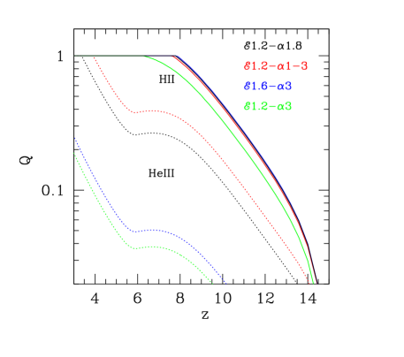
Figure 1: The evolution of the filling factor calculated for four of the reionisation models listed in Table 1. The black, red, blue and green curves correspond to model ${\mathcal{E}}$1.2-$\alpha$1.8, ${\mathcal{E}}$1.2-$\alpha$1-3, ${\mathcal{E}}$1.6-$\alpha$3 and ${\mathcal{E}}$1.2-$\alpha$3, while the solid and dotted curves display the H$\,\rm\scriptstyle II\$and He$\,\rm\scriptstyle III\$filling factors, respectively.

We next define the redshift evolution of the total comoving hydrogen ionising emissivity as:

$${\epsilon}_{\rm HI}=\left\{\begin{array}[]{ll}{\mathcal{E}}\times 10^{50.89+{\rm log}(\chi(z))}\frac{\alpha^{-1}(\alpha_{\rm b}+3)}{2}&z>6,\\ {\mathcal{E}}\times 10^{50.50-0.06(z-6)}\frac{\alpha^{-1}(\alpha_{\rm b}+3)}{2}&z\leq 6,\\ \end{array}\right.$$ (3)

with

$$\chi(z)=\frac{\xi{\rm e}^{\zeta(z-9)}}{\left(\xi-\zeta+\zeta{\rm e}^{\xi(z-9)}\right)}.$$ (4)

Here ${\mathcal{E}}$ is a free parameter which sets the amplitude of the emissivity, $\xi=14/15$, $\zeta=2/3$, $\alpha$ is the extreme-UV (EUV) power-law spectral index of the sources and $\alpha_{\rm b}$ is the spectral index of the ionising background; we shall assume the same value for both. Eq. (3) is consistent with observational constraints on the H$\,\rm\scriptstyle I\$photo-ionisation rate from the Ly$\alpha$ forest at $z\leq 6$ (Bolton & Haehnelt 2007, see also Section 6.2) and the mean free path for Lyman limit photons (Songaila & Cowie 2010), while Eq. (4) (Springel & Hernquist 2003) provides a simple parameterisation for the rising emissivity at $z>6$ (peaking at $z=9$) required by the Ly$\alpha$ forest data (e.g. Bolton & Haehnelt 2007; Pritchard et al. 2010).

We shall consider three different models for the spectral shape of the ionising emission, all of which achieve H$\,\rm\scriptstyle I\$reionisation by $z\geq 6$ (i.e. $Q_{\rm HII}\sim 1$). Our reference models (${\mathcal{E}}$1.2-$\alpha$1.8 and ${\mathcal{E}}$1.6-$\alpha$3) assume $\alpha=1.8$ and $\alpha=3$, while a third model (${\mathcal{E}}$1.2-$\alpha$1-3) assumes 30 (70) per cent of the sources have $\alpha=1$ (3). A spectral index of $\alpha=1.8$ is typical of quasars (Telfer et al. 2002), while $\alpha=3$ is consistent with star forming galaxies with metallicities close to solar, i.e. population-II stellar sources (Leitherer et al. 1999). The third model assumes that a fraction of the sources instead have rather hard spectra, $\alpha=1$, typical of hard quasars or population-III stars (e.g. Bromm et al. 2001b).

In Figure 1, the evolution of both $Q_{\rm HII}$ (solid curves) and $Q_{\rm HeIII}$ (dotted curves) is shown for model ${\mathcal{E}}$1.2-$\alpha$1.8 (black curves), ${\mathcal{E}}$1.2-$\alpha$1-3 (red curves) and ${\mathcal{E}}$1.6-$\alpha$3 (blue curves). The models are normalised to have similar comoving hydrogen ionising emissivities at each redshift, ensuring that any differences in the reionisation histories are largely due to the different EUV spectral indices. For example, He$\,\rm\scriptstyle II\$reionisation is completed ($Q_{\rm HeIII}\sim 1$) progressively later in models ${\mathcal{E}}$1.2-$\alpha$1.8 and ${\mathcal{E}}$1.6-$\alpha$3, which have softer ionising spectra compared to ${\mathcal{E}}$1.2-$\alpha$1-3.

Finally, in addition to these three reference reionisation histories, we shall also consider two further models; ${\mathcal{E}}$1.2-$\alpha$1.8-H which excludes the treatment of helium, and ${\mathcal{E}}$1.2-$\alpha$3 which results in a late H$\,\rm\scriptstyle I\$reionisation at $z\simeq 6$. We include the latter to explore the possibility that the volume weighted neutral fraction in the IGM at $z\simeq 7$ may be greater than 10 per cent. Such a substantial neutral fraction is suggested by recent observations, which, if confirmed by future investigations, may be in tension with models which satisfy constraints on the Thomson scattering optical depth and the hydrogen photo-ionisation rate (see Section 6 later for further details). The parameters for these reionisation models are summarised in Table 1. Using these simple emissivity models, we now turn to describing our cosmological radiative transfer simulations.

Table 1: Summary of the ionising emissivity models used in this work. The columns indicate, from left to right, the name of the model, the amplitude of the emissivity, ${\mathcal{E}}$, the assumed EUV spectral index of the source spectrum, $\alpha$, and the percentage of sources with that spectrum, $f_{\alpha}$. The final column indicates whether or not helium has been included in the simulations.

Model	${\mathcal{E}}$	$\alpha$	$f_{\alpha}$ [%]	He
${\mathcal{E}}$1.2-$\alpha$1.8-H	1.2	1.8	100	No
${\mathcal{E}}$1.2-$\alpha$1.8	1.2	1.8	100	Yes
${\mathcal{E}}$1.2-$\alpha$1-3	1.2	1 (3)	30 (70)	Yes
${\mathcal{E}}$1.6-$\alpha$3	1.6	3	100	Yes
${\mathcal{E}}$1.2-$\alpha$3	1.2	3	100	Yes

3 Numerical simulations

3.1 Hydrodynamical simulations

In order to perform our reionisation simulations, we require a model for the intergalactic medium. In this work we use a hydrodynamical simulation performed in a comoving cubic box of size $35.12h^{-1}\rm\,Mpc$. The simulation was performed using the parallel smoothed particle hydrodynamics (SPH) code GADGET-3, which is an updated version of the publicly available code GADGET-2 (Springel 2005). A total of $2\times 512^{3}$ dark matter and gas particles were followed in the simulation, yielding a mass per gas particle of $4.15\times 10^{6}h^{-1}\rm\,M_{\odot}$. Beginning at $z=16$, outputs were obtained from the simulation at redshift intervals $\Delta z=0.5$ until $z=7$, and then at $\Delta z=0.4$ intervals until $z=5$. Haloes were identified at each redshift using a friend-of-friends halo finding algorithm with a linking length of $0.2$. Star formation was included using a simplified prescription which converts all gas particles with overdensity $\Delta=\rho/\langle\rho\rangle>10^{3}$ and temperature $T<10^{5}\rm~{}K$ into collisionless stars. Note that because of this simple treatment our simulations do not self-consistently model star formation and feedback. Instead, as discussed in Section 2, we shall model the ionising emissivity during reionisation using our empirically motivated prescription.

The hydrodynamical simulation also includes the photo-ionisation and heating of the IGM by a spatially uniform ionising background (Haardt & Madau 2001). This model assumes the IGM is optically thin, and that the IGM is reionised instantaneously at $z=9$. Although we shall recompute the IGM ionisation and thermal state with our radiative transfer (RT) simulations at all redshifts, including the UV background in the hydrodynamical simulation at $z<9$ is nevertheless important for properly modelling the gas distribution. The photo-heating significantly reduces the clumping factor of the gas in the hydrodynamical simulation due to pressure smoothing (Pawlik et al. 2009), and without this feedback effect the simulation would over-predict the gas clumping factor towards the end of reionisation. On the other hand, we note that increasing the mass resolution of our simulations would increase the clumping factor and hence the rate of recombination in the simulations. However, we defer a detailed investigation of the clumping factor to a future study. It should be noted though that, while the inclusion of a clumping factor assures a better estimate of the gas recombination rate, it does not capture all the relevant radiative transfer effects, such as self-shielding.

3.2 Radiative transfer simulations

Once the hydrodynamical simulation outputs were obtained, the gas number densities, $n$, temperatures, $T$ (at $z>9$ only, see Section 3.1) and the halo masses, $M$, were transferred to a $128^{3}$ grid for the RT calculations, which are performed as a post-process. The gridded densities and temperatures are obtained by assigning the particle data to a regular grid using the SPH kernel (e.g. Monaghan 1992). The corresponding grid for the halo masses is obtained by using the cloud-in-cell algorithm (Hockney & Eastwood 1988) to assign the haloes identified by the friends-of-friends algorithm to a regular grid with the same dimensions.

The RT is followed using the code CRASH (Ciardi et al., 2001; Maselli et al., 2003, 2009; Partl et al., 2011), which self-consistently calculates the evolution of the hydrogen and helium ionisation state and the gas temperature. CRASH is a Monte Carlo based ray tracing scheme, where the ionising radiation and its time varying distribution in space is represented by multi-frequency photon packets which travel through the simulation volume. For further details regarding the radiative transfer implementation we refer the reader to the original CRASH papers. For each output $i$ of the hydrodynamical simulation, the RT is followed for a time $t_{\rm rt,i}=t_{\rm H}(z_{\rm i+1})-t_{\rm H}(z_{\rm i})$, where $t_{\rm H}(z_{\rm i})$ is the Hubble time corresponding to $z_{\rm i}$ which is the redshift of output $i$. The gas number density is updated at each hydrodynamical simulation snapshot, and between two snapshots it is evolved as $n(x_{\rm c},y_{\rm c},z_{\rm c})(z)=n(x_{\rm c},y_{\rm c},z_{\rm c})(z_{\rm i})(1+z)^{3}/(1+z_{\rm i})^{3}$, where $(x_{\rm c},y_{\rm c},z_{\rm c})$ are the coordinates of cell $c$ and $z_{\rm i}>z>z_{\rm i+1}$. Although the current implementation of CRASH is able to model diffuse radiation without approximations, in this work we choose to use the on-the-spot approximation. The infinite velocity of light approximation is made and a photon packet is considered as lost once it has exited the simulation box, i.e. we do not use periodic boundary conditions.

The emission properties of the sources are derived as follows. Guided by our semi-analytical calculations in Section 3.1, we assume that the total comoving hydrogen ionising emissivity at each redshift is given by Eqs. (3) and (4). Thus, the total rate of ionising photons emitted at each output of the hydrodynamical simulation is given by $\dot{N}_{\rm i}=\epsilon_{\rm HI}(z_{\rm i})V_{\rm com}$, where $V_{\rm com}$ is the comoving volume of the simulation. The emissivity, $\dot{N}_{\rm i}$, is then distributed among the sources according to their gas mass, i.e. $\dot{N}_{\rm i,j}=\dot{N}_{\rm i}M_{\rm j}/M_{\rm tot,i}$, where $j$ refers to the source and $M_{\rm tot,i}$ is the total gas mass of sources at output $i$. This method of assigning the emissivity avoids assuming an escape fraction of ionising photons and a star formation efficiency, which are very uncertain parameters. Furthermore, as already discussed this empirical approach is designed to be consistent with the existing observational constraints on the photo-ionisation rate at $z\sim 6$. Depending on the redshift and number of sources, we emit $10^{5}-10^{6}$ photon packets per source at each $t_{\rm rt,i}$, corresponding to a total of $\sim 5\times 10^{7}-10^{10}$ photon packets. At $z<8.5$ the total number is always $>10^{9}$, assuring convergence of the results to less than one percent (in relative terms) in the ionisation and neutral fraction for all the species, as well as the gas temperature (see the appendix for further details).

The ionisation fraction in the RT simulations is initialised to its equilibrium value at $z_{\rm in}$, while the initial gas temperatures correspond to those predicted by the hydrodynamical simulation, and remain so until either a cell is crossed by a photon packet or at redshifts $z<9$. In the latter instance, the temperature is held fixed at the $z=9$ value, prior to the onset of photo-heating in the hydrodynamical simulation. Once a cell is crossed by a photon packet, the ionisation fraction and gas temperature are then updated self-consistently within the radiative transfer calculation.

We have performed five RT simulations in total in this study, using the models summarised in Table 1. In order to assess the effect of including helium on the evolution of hydrogen reionisation, in model ${\mathcal{E}}$1.2-$\alpha$1.8-H we include only hydrogen with a fraction by mass (number) of 0.742 (0.92). Furthermore, in model ${\mathcal{E}}$1.2-$\alpha$1-3, where there are two populations of ionising sources with different power-law spectra, the EUV spectral indices are assigned to sources randomly (i.e. no correlation with the halo mass is assumed) to reproduce the correct relative proportions. Note also that in all five models the power-law ionising spectra extend to a maximum frequency of $\sim 200$ eV and that the contribution from X-rays is not included. Finally, due to the large number of sources present in the box, to reduce the computational time we adopt the clustering technique described and tested in Pierleoni et al. (in prep). This approach significantly speeds up our simulations; for reference, the number of sources in the $35.12h^{-1}$ Mpc box is reduced from 68 (80597) to 34 (14112) at $z=15$ (8).

4 Empirical calibration of the reionisation simulations

Before proceeding to discuss the results of our simulations in detail, we first compare them to the two key observables we deliberately calibrate to; the electron scattering optical depth and the background photo-ionisation rate at $z\sim 6$ inferred from the Ly$\alpha$ forest. As mentioned in Section 2, our choice for the reionisation histories in the simulations is such that these key observational constraints should automatically be satisfied.

4.1 The Thomson scattering optical depth

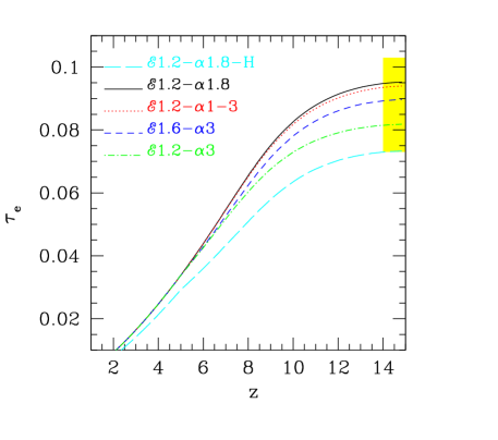
Figure 2: The Thomson scattering optical depth computed from each of our five radiative transfer simulations: ${\mathcal{E}}$1.2-$\alpha$1.8-H (cyan long dashed line), ${\mathcal{E}}$1.2-$\alpha$1.8 (black solid), ${\mathcal{E}}$1.2-$\alpha$1-3 (red dotted), ${\mathcal{E}}$1.6-$\alpha$3 (blue dashed) and ${\mathcal{E}}$1.2-$\alpha$3 (green dotted dashed). The shaded area corresponds to the 7-yr WMAP value of $0.088\pm 0.015$ (Komatsu et al., 2011).

We first consider the observational constraint on the integrated reionisation history, in the form of the Thomson scattering optical depth, $\tau_{\rm e}$. In Figure 2 the evolution of $\tau_{e}$ is shown for all five of our RT simulations, together with the value measured by the 7-yr WMAP mission, $0.088\pm 0.015$ (Komatsu et al., 2011). The optical depth, $\tau_{e}$, is calculated from the RT simulations as:

$$\tau_{e}=c\sigma_{\rm T}\int n_{\rm e}(t)dt,$$ (5)

where $c$ is the speed of light, $\sigma_{\rm T}=6.65\times 10^{-25}$ cm² is the Thomson scattering cross section, $n_{\rm e}=n_{\rm HII}+n_{\rm HeII}+2n_{\rm HeIII}$ is the electron number density in units of cm^-3 and $n_{\rm i}$ is the number density of species $i$, with $i$=H$\,\rm\scriptstyle II\$, He$\,\rm\scriptstyle II\$and He$\,\rm\scriptstyle III$. Here $n_{\rm e}$ is evaluated directly from the simulations for $z>z_{\rm min}=5$, which is the redshift at which the radiative transfer simulations are stopped. At lower redshift, where we do not have simulation outputs, we instead calculate $n_{\rm e}$ analytically assuming that: (i) the average density equals the cosmological mean density; (ii) hydrogen is completely ionised; (iii) $x_{\rm{HeII}}=1$ ($x_{\rm{HeIII}}=0$) for $3<z<z_{\rm min}$ and $x_{\rm{HeII}}=0$ ($x_{\rm{HeIII}}=1$) for $z<3$.

The Thomson scattering optical depth calculated in this manner has a value of 0.073, 0.095, 0.094, 0.090, 0.081 for the simulations ${\mathcal{E}}$1.2-$\alpha$1.8-H, ${\mathcal{E}}$1.2-$\alpha$1.8, ${\mathcal{E}}$1.2-$\alpha$1-3, ${\mathcal{E}}$1.6-$\alpha$3 and ${\mathcal{E}}$1.2-$\alpha$3, respectively. As expected, these values are consistent with those measured by the WMAP satellite (Komatsu et al., 2011). Note, however, that for model ${\mathcal{E}}$1.2-$\alpha$1.8-H we consider only the contribution from hydrogen. The inclusion of helium in these models is clearly important, adding an additional $\tau_{\rm e}\sim 0.02$ to the total optical depth for ${\mathcal{E}}$1.2-$\alpha$1.8. This is largely because of the extra electrons liberated by the reionisation of helium, but will also be partly due to the higher IGM temperatures which arise from He$\,\rm\scriptstyle II\$photo-heating; the temperature dependence of the H$\,\rm\scriptstyle II\$recombination rate, $\alpha_{\rm HII}\propto T^{-0.7}$, means higher temperatures will produce a slight increase in the H$\,\rm\scriptstyle II\$fraction and hence the electron number density.

4.2 The background photo-ionisation rate

The photo-ionisation rates are compared to the observational data in Figure 3. This comparison, however, is less straightforward for two reasons. Firstly, the photo-ionisation rate is not a direct output from our RT simulations, and so we must estimate it indirectly by assuming ionisation equilibrium in each cell $(x_{\rm c},y_{\rm c},z_{\rm c})$, such that:

$$\Gamma_{\rm HI}=\alpha_{\rm HII}(T)\frac{n_{\rm e}n_{\rm HII}}{n_{\rm HI}}-\gamma_{\rm eHI}(T)n_{\rm e},$$ (6)

where $\alpha_{\rm HII}$ and $\gamma_{\rm eHI}$ are the hydrogen recombination and collisional ionisation rate in units of $\rm cm^{3}\,s^{-1}$, respectively. All the other quantities have their usual meaning. This will be a reasonable approximation for most of the cells in our simulation volume after they have been reionised, but will break down close to reionisation when non-equilibrium effects are important. Secondly, the observational constraints on the photo-ionisation rate are derived from the Ly$\alpha$ absorption observed in $z\simeq 6$ quasar spectra (e.g. Fan et al. 2006; Bolton & Haehnelt 2007; Calverley et al. 2011). The transmitted Ly$\alpha$ flux at these redshifts preferentially samples highly ionised, underdense regions in the IGM, and so we must take care to use similar criteria when comparing to volume averaged values in the simulations.

In the upper panel of Figure 3 the evolution of the volume averaged H$\,\rm\scriptstyle I\$photo-ionisation rate, $\Gamma_{\rm HI}$, is shown for model ${\mathcal{E}}$1.2-$\alpha$3. The different curves display $\Gamma_{\rm HI}$ for a variety of different sub-samples drawn from the simulation volume. The black solid curve shows the photo-ionisation rate for all cells, whereas the dotted red curve displays the data for underdense cells ($\Delta<1$) only. The remaining three curves again show the photo-ionisation rate in underdense cells, but now with the additional condition that $x_{\rm HI}<10^{-2}$ (blue dashed), $10^{-3}$ (green dot-dashed) and $10^{-4}$ (cyan long dashed). These cuts correspond to $\sim 0.13$, $0.13$, $0.84$ per cent of the total number of cells in the simulation volume at $z=14$. At $z=6$ the percentages are instead 63, 62, and 18, respectively. When all cells are included, the evolution of $\Gamma_{\rm HI}$ rises to a peak at $z\sim 8$ (following the rising emissivity at $z>6$ in Eq. 4) but declines toward higher redshift. This is because a larger number of neutral cells are present toward higher redshifts, lowering the volume averaged photo-ionisation rate. The average photo-ionisation rate is slightly lower if only underdense cells are included because the overdense (and hence first to reionise) regions are discarded. In other words, the photo-ionisation rates are higher in the overdense cells since the ionising radiation is correlated with the underlying density field (see also Iliev et al. 2008; Mesinger & Furlanetto 2009).

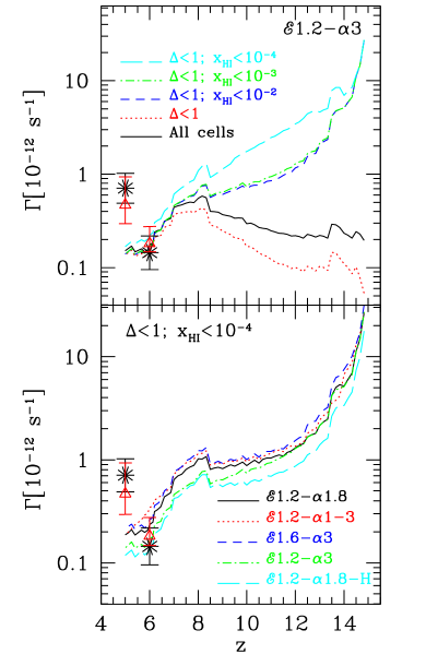
Figure 3: Upper panel: The redshift evolution of the volume averaged photo-ionisation rate, $\Gamma_{\rm HI}$, for model ${\mathcal{E}}$1.2-$\alpha$3. The black solid curve shows the photo-ionisation rate for all cells, while the dotted red curve displays the data for underdense cells ($\Delta<1$) only. The remaining three curves show the photo-ionisation rate in underdense cells, but now with the additional condition that $x_{\rm HI}<10^{-2}$ (blue dashed), $10^{-3}$ (green dot-dashed) and $10^{-4}$ (cyan long dashed). Lower panel: The redshift evolution of the volume averaged $\Gamma_{\rm HI}$ for cells with overdensity $\Delta<1$ and $x_{\rm HI}<10^{-4}$ only. The curves correspond to the models ${\mathcal{E}}$1.2-$\alpha$1.8-H (cyan long dashed lines), ${\mathcal{E}}$1.2-$\alpha$1.8 (black solid), ${\mathcal{E}}$1.2-$\alpha$1-3 (red dotted), ${\mathcal{E}}$1.6-$\alpha$3 (blue dashed) and ${\mathcal{E}}$1.2-$\alpha$3 (green dotted-dashed). In all panels the triangles and stars display respectively the observational constraints from the Ly$\alpha$ forest (Wyithe & Bolton, 2011) and the proximity effect (Calverley et al., 2011).

At $z=6$, by which time all the underdense regions in the simulation have been reionised, all curves converge to a similar value. Note, however, that in the cases where cuts in the neutral fraction are also applied, at $z>6$ the photo-ionisation rate is always higher compared to the average for all the underdense cells (red dotted curve). This is in part because the averages are, by definition, only for highly ionised cells which are assumed to be in ionisation equilibrium. The difference is more pronounced at $z>8$, however, when the ionised regions probed are the increasingly rare ionised bubbles around sources. We thus also expect higher photo-ionisation rates because the selected cells are closer to the ionising sources. However, these regions are rare and so only provide a small contribution to the overall volume averaged ionisation rate.

In the lower panel of Figure 3 the evolution of the volume averaged $\Gamma_{\rm HI}$ is shown for all five simulations in underdense cells which are highly ionised only ($x_{\rm HI}<10^{-4}$). Note that this cut most closely represents the regions of the IGM from which the photo-ionisation rates are measured at $z\simeq 6$ (Bolton & Haehnelt 2007). The redshift evolution of $\Gamma_{\rm HI}$ is, as might be expected, similar for all models. Model ${\mathcal{E}}$1.2-$\alpha$3 typically gives a smaller photo-ionisation rate due to the lower normalisation of the emissivity. On the other hand, model ${\mathcal{E}}$1.2-$\alpha$1.8-H always has a slightly lower value of $\Gamma_{\rm HI}$ compared to the case including helium, ${\mathcal{E}}$1.2-$\alpha$1.8. Note, however, the photoionisation rates are inferred from Eq. (6) rather than directly obtained, and so variations in the gas temperature and electron number density in this model will be partly responsible for this difference.

Finally, as required, we find that for all models at $z=6$ the photo-ionisation rates are consistent with the observational constraints from the Ly$\alpha$ forest (Wyithe & Bolton 2011) and proximity effect (Calverley et al. 2011), represented by triangles and stars with error bars in Figure 3, respectively. On the other hand, the photo-ionisation rates at $z=5$ underpredict the observed values by a factor of $2$–$3$, despite the fact we have deliberately used an ionising emissivity which agrees with these data when assuming a mean free path consistent with recent observational measurements (e.g. Songaila & Cowie 2010). This discrepancy may be understood by recalling that $\Gamma_{\rm HI}\propto\epsilon_{\rm HI}\lambda_{\rm HI}$, where $\lambda_{\rm HI}$ is the mean free path at the Lyman limit. Assuming a power-law slope for the H$\,\rm\scriptstyle I\$column density distribution of $\beta=1.3$, Songaila & Cowie (2010) measure $\lambda_{\rm HI}\simeq 84$ (49) comoving Mpc at $z=5$ (6). In comparison, our simulation volume is $48.7$ comoving Mpc on a side. This sets an effective upper limit on the mean free path of ionising photons in our simulations which is around half the observed value at $z=5$. Our small simulation box therefore most likely accounts for this apparent discrepancy, and we caution that the ionising emissivity in our simulations is underestimated at $z<6$ as a result.

5 The evolution of the IGM ionisation and thermal state

We have found that our simulations are in reasonable agreement with both the observed Thomson scattering optical depth and background photo-ionisation rate at $z=6$, giving us confidence that we may now explore the implications of these models for the ionisation and thermal state of the IGM in further detail.

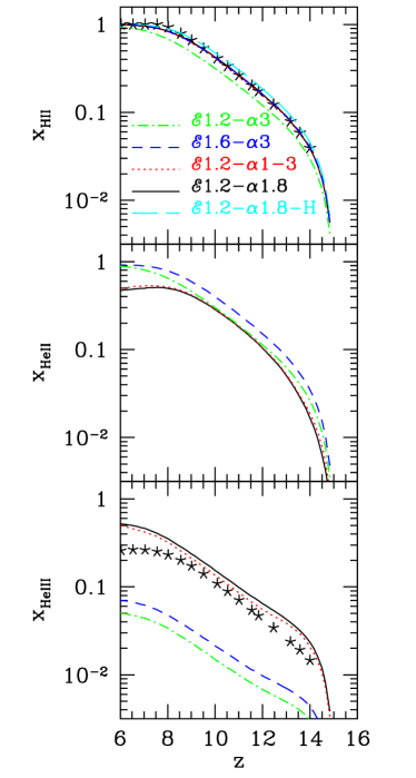
Figure 4: Upper panel: The evolution of the volume averaged H$\,\rm\scriptstyle II\$fraction calculated with the radiative transfer simulations for models ${\mathcal{E}}$1.2-$\alpha$1.8-H (long dashed cyan line), ${\mathcal{E}}$1.2-$\alpha$1.8 (solid black lines), ${\mathcal{E}}$1.2-$\alpha$1-3 (dotted red), ${\mathcal{E}}$1.6-$\alpha$3 (dashed blue) and ${\mathcal{E}}$1.2-$\alpha$3 (dot-dashed green). Note the solid black, dotted red, and dashed blue lines are almost indistinguishable. The stars display the semi-analytic result for model ${\mathcal{E}}$1.2-$\alpha$1.8 (see Section 2.2 for details). Middle panel: As for the upper panel but for the volume averaged He$\,\rm\scriptstyle II\$fraction. Note that in this case model ${\mathcal{E}}$1.2-$\alpha$1.8-H is not present. Lower panel: As for the upper middle but for the volume averaged He$\,\rm\scriptstyle III\$fraction. The stars again refer to the semi-analytic result for model ${\mathcal{E}}$1.2-$\alpha$1.8.

5.1 The ionisation fraction

The volume averaged ionisation fractions predicted by the RT simulations are displayed in Figure 4, where the upper, middle and lower panels refer, respectively, to the evolution of the H$\,\rm\scriptstyle II$, He$\,\rm\scriptstyle II\$and He$\,\rm\scriptstyle III\$fractions for the models summarized in Table 1. Reionisation is largely complete by $z=7$ in all models (i.e. $x_{\rm HI}\leq 0.05$), with the exception of ${\mathcal{E}}$1.2-$\alpha$3, which has an H$\,\rm\scriptstyle I\$fraction of 0.15 at $z=7$.

Although the aim of this study is not to compare the RT simulations with the semi-analytic calculations used to guide our choice of ionising emissivity, it is interesting to note that the numerical models reproduce the semi-analytic results for the H$\,\rm\scriptstyle II\$evolution remarkably well. However, the agreement is to some extent a fortunate coincidence; a different assumption for the hydrogen clumping factor in H$\,\rm\scriptstyle II\$regions, $C_{\rm HII}$, or IGM temperature in the semi-analytical model would worsen the agreement. The agreement between the numerical and semi-analytical evolution of $x_{\rm HeIII}$ is slightly poorer, which is indeed most likely due to slightly different values for the clumping factor and/or temperature in the two approaches. Nevertheless, the general agreement indicates that semi-analytical approaches are indeed useful for quickly exploring parameter space in reionisation models, at least in terms of the volume of the IGM which is ionised. This is perhaps not too surprising; both calculations are effectively just counting ionising photons and recombinations. Indeed, “semi-numerical” schemes which additionally follow the topology of reionisation are also in relatively good agreement with the results of full RT calculations (e.g. Zahn et al. 2011).

The long dashed cyan curve in the top panel of Figure 4 compares the ${\mathcal{E}}$1.2-$\alpha$1.8-H model, which excludes helium, to the corresponding reference run ${\mathcal{E}}$1.2-$\alpha$1.8. The abundance of H$\,\rm\scriptstyle II\$in ${\mathcal{E}}$1.2-$\alpha$1.8-H is slightly higher because all of the ionising photons ($>13.6\,\rm eV$) are used to ionise hydrogen. The inclusion of helium in model ${\mathcal{E}}$1.2-$\alpha$1.8 has a small effect on the evolution of the neutral hydrogen fraction, as some of the hydrogen ionising photons with energies $>24.6\,\rm eV$ are now used to reionise He$\,\rm\scriptstyle I$. However, the difference between $x_{\rm HII}$ in the ${\mathcal{E}}$1.2-$\alpha$1.8-H and ${\mathcal{E}}$1.2-$\alpha$1.8 models is never above a few per cent.

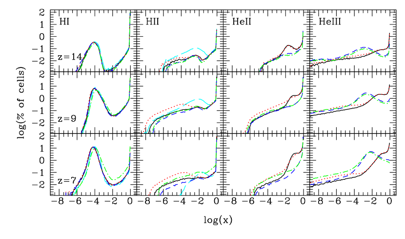
Figure 5: The percentage of cells in the radiative transfer simulations as a function H$\,\rm\scriptstyle I$, H$\,\rm\scriptstyle II$, He$\,\rm\scriptstyle II$ and He$\,\rm\scriptstyle III$ fractions (from left to right) at $z$=14 (upper row), 9 (middle row) and 7 (lower row). The curves in each panel correspond to a different reionisation history: ${\mathcal{E}}$1.2-$\alpha$1.8-H (long dashed cyan, first two columns only), ${\mathcal{E}}$1.2-$\alpha$1.8 (solid black), ${\mathcal{E}}$1.2-$\alpha$1-3 (dotted red), ${\mathcal{E}}$1.6-$\alpha$3 (dashed blue) and ${\mathcal{E}}$1.2-$\alpha$3 (dot-dashed green).

The impact of different spectral energy distributions on the ionised fractions can be seen by comparing model ${\mathcal{E}}$1.2-$\alpha$1.8 to models ${\mathcal{E}}$1.2-$\alpha$1-3 and ${\mathcal{E}}$1.6-$\alpha$3. Interestingly, for the mixed source model ${\mathcal{E}}$1.2-$\alpha$1-3, all three ionisation fractions (H$\,\rm\scriptstyle II$, He$\,\rm\scriptstyle II$, He$\,\rm\scriptstyle III$) are extremely similar to those of model ${\mathcal{E}}$1.2-$\alpha$1.8. This is because both the comoving emissivity and the number of photons with frequencies above the helium ionisation thresholds are very similar in the two models. Spectra with power-law indices $\alpha=1$, 1.8 and 3 have a percentage of ionising photons above the He$\,\rm\scriptstyle I\$(He$\,\rm\scriptstyle II$) ionisation threshold, i.e. above 24.6 eV (54.4 eV), of $\sim 52$ (19.5), 34 (7.5) and 17 (1.5) per cent, respectively. In the case of the models with the softer ionising spectrum (i.e. $\alpha=3$), $x_{\rm HeIII}$ is much lower due to the paucity of higher energy photons. The softer spectrum is also reflected in the evolution of $x_{\rm HeII}$, which is very similar to that of $x_{\rm HII}$.

Finally, model ${\mathcal{E}}$1.2-$\alpha$3 exhibits very similar behaviour to that of ${\mathcal{E}}$1.6-$\alpha$3 because they have the same spectral index, but the ionisation fractions at the same redshift are smaller due to the lower amplitude of the comoving emissivity. Note, however, that both of these models have EUV spectral indices which are too soft to complete He$\,\rm\scriptstyle II\$reionisation by $z\simeq 2.5$–$3$ (e.g. Fig. 1). These models are therefore likely inconsistent with the He$\,\rm\scriptstyle II\$Ly$\alpha$ forest data at $z\simeq 3$ (e.g. Shull et al. 2010; Worseck et al. 2011; Syphers et al. 2011) unless the ionising background spectral shape hardens at $z<6$, perhaps due to the increasing contribution of quasars to the ionising background. For reference, the volume averaged ionisation fractions at $z=14,\,9,\,7$ and 6 are summarised in Table 2.

Table 2: Summary of the volume averaged ionisation fractions and temperature within the RT simulations. The columns indicate, from left to right, the name of the model, the redshift $z$, the volume averaged ionisation fractions $x_{\rm HII}$, $x_{\rm HeII}$ and $x_{\rm HeIII}$, and the volume averarged temperature $T$.

Model	$z$	$x_{\rm HII}$	$x_{\rm HeII}$	$x_{\rm HeIII}$	$T$ [K]
	14	0.045	–	–	918
	9	0.695	–	–	9760
${\mathcal{E}}$1.2-$\alpha$1.8-H	7	0.981	–	–	11047
	6	0.998	–	–	10224
	14	0.038	0.017	0.023	820
	9	0.632	0.410	0.238	10464
${\mathcal{E}}$1.2-$\alpha$1.8	7	0.960	0.499	0.464	16594
	6	0.993	0.472	0.522	16998
	14	0.038	0.019	0.021	804
	9	0.618	0.419	0.211	10190
${\mathcal{E}}$1.2-$\alpha$1-3	7	0.953	0.531	0.425	16565
	6	0.993	0.490	0.504	17454
	14	0.039	0.035	0.004	643
	9	0.627	0.594	0.032	7674
${\mathcal{E}}$1.6-$\alpha$3	7	0.957	0.894	0.063	11425
	6	0.993	0.922	0.070	11347
	14	0.029	0.026	0.003	488
	9	0.481	0.459	0.023	6020
${\mathcal{E}}$1.2-$\alpha$3	7	0.852	0.807	0.044	10643
	6	0.938	0.888	0.050	11347

A more quantitative representation of the distributions of the various ionised fractions is displayed in Figure 5, where from left to right the percentage of cells as a function of $x_{\rm HI}$, $x_{\rm HII}$, $x_{\rm HeII}$ and $x_{\rm HeIII}$ are shown for the five reionisation models at $z=14$ (upper row), 9 (middle row) and 7 (lower row). At the highest redshifts most of the hydrogen is in a neutral state, but as the redshift decreases and reionisation proceeds the percentage of ionised cells increases for all models. During the final stages of reionisation (represented here at $z=7$), most of the cells will be fully or almost fully ($x_{\rm HII}>0.9$) ionised and, as a consequence, the percentage of cells with a lower ionisation fraction decreases again. Model ${\mathcal{E}}$1.2-$\alpha$1.8-H generally has a slightly higher number of highly ionised cells compared to the three reference models. This is again because helium is absent in this model; all the ionising photons are thus absorbed by hydrogen, enabling hydrogen reionisation to proceed slightly more quickly. The behaviour of models ${\mathcal{E}}$1.6-$\alpha$3 and ${\mathcal{E}}$1.2-$\alpha$1-3 is also rather similar to ${\mathcal{E}}$1.2-$\alpha$1.8, except ${\mathcal{E}}$1.6-$\alpha$3 (${\mathcal{E}}$1.2-$\alpha$1-3) has slightly less (more) cells with very small ionised fractions. This is because of the softer (harder) ionising spectra which produce proportionally more (less) hydrogen ionising photons. As noted previously, the He$\,\rm\scriptstyle II\$and He$\,\rm\scriptstyle III\$ionisation fractions for ${\mathcal{E}}$1.2-$\alpha$1-3 and ${\mathcal{E}}$1.2-$\alpha$1.8 show rather similar behaviour, while ${\mathcal{E}}$1.6-$\alpha$3 exhibits much smaller He$\,\rm\scriptstyle III\$fractions due to the presence of fewer hard, helium ionising photons. A situation similar to model ${\mathcal{E}}$1.6-$\alpha$3 applies to ${\mathcal{E}}$1.2-$\alpha$3, with the difference that the lower emissivity means reionisation is less advanced.

From this analysis it is clear that including intergalactic helium and a treatment of multi-frequency radiative transfer has a rather small effect on the ionisation state of hydrogen during reionisation. However, the hard ionising photons capable of ionising helium will also significantly photo-heat the IGM. We therefore now turn to consider the effect on the thermal state of the IGM at high redshift.

5.2 The volume averaged temperature

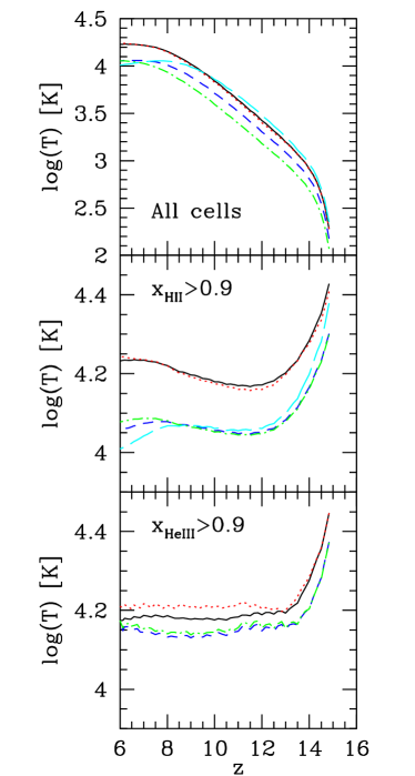
Figure 6: Redshift evolution of the volume averaged temperature. The curves correspond to models ${\mathcal{E}}$1.2-$\alpha$1.8-H (long dashed cyan), ${\mathcal{E}}$1.2-$\alpha$1.8 (solid black), ${\mathcal{E}}$1.2-$\alpha$1-3 (dotted red), ${\mathcal{E}}$1.6-$\alpha$3 (dashed blue) and ${\mathcal{E}}$1.2-$\alpha$3 (dotted-dashed green) respectively. Upper panel: The temperature calculated by averaging over all the cells in the simulation volume. Middle panel: The temperature calculated by averaging over only those cells with $x_{\rm HII}>0.9$. Lower panel: The temperature calculated by averaging over only on those cells with $x_{\rm HeIII}>0.9$.

The redshift evolution of the volume averaged gas temperature in our five reionisation models is displayed in the upper panel of Figure 6. This quantity will depend on the volume of the IGM already reionised at any given redshift, as well as the spectral shape of the sources in the simulation and whether or not helium photo-heating is included. The first point to note is that at early times ($z>10$) model ${\mathcal{E}}$1.2-$\alpha$1.8-H has a volume averaged gas temperature which is $\sim$10 per cent higher than the corresponding model with helium, ${\mathcal{E}}$1.2-$\alpha$1.8. This is due to the slightly larger volume of the IGM in which hydrogen is photo-ionised and heated compared to the other models. This arises from the fact (as discussed earlier) that no hydrogen ionising photons are used to ionise neutral helium. Note, however, that by $z\sim 10$ the inclusion of He$\,\rm\scriptstyle II\$photo-ionisation results in a higher average temperature for ${\mathcal{E}}$1.2-$\alpha$1.8 compared to ${\mathcal{E}}$1.2-$\alpha$1.8-H. In addition, in the absence of any additional heating from He$\,\rm\scriptstyle II\$photo-ionisation, the temperature for ${\mathcal{E}}$1.2-$\alpha$1.8-H slightly declines at $z<9$ as the IGM cools.

The volume averaged temperature evolution does not exhibit any substantial difference between models ${\mathcal{E}}$1.2-$\alpha$1.8 and ${\mathcal{E}}$1.2-$\alpha$1-3, which is expected from the very similar behaviour of the ionisation fractions discussed earlier. On the other hand, despite having a similar behaviour for the evolution of the H$\,\rm\scriptstyle II\$filling factor, the softer ionising spectrum used by ${\mathcal{E}}$1.6-$\alpha$3 produces temperatures 20-30 per cent lower than ${\mathcal{E}}$1.2-$\alpha$1.8. This is partly because the volume filling factor of He$\,\rm\scriptstyle III\$is smaller in this model, but also because the softer spectrum results in less energy (and hence photo-heating) per photo-ionisation on average. Lastly, for the case of ${\mathcal{E}}$1.2-$\alpha$3, the volume averaged temperature is $\sim$20–25 per cent lower compared to model ${\mathcal{E}}$1.6-$\alpha$3 over most of reionisation, but converges to a similar temperature by $z=6$. This is due to the lower ionising emissivity, and hence smaller filling factor of ionised hydrogen, used in model ${\mathcal{E}}$1.2-$\alpha$3 which delays the completion of hydrogen reionisation to $z\simeq 6$.

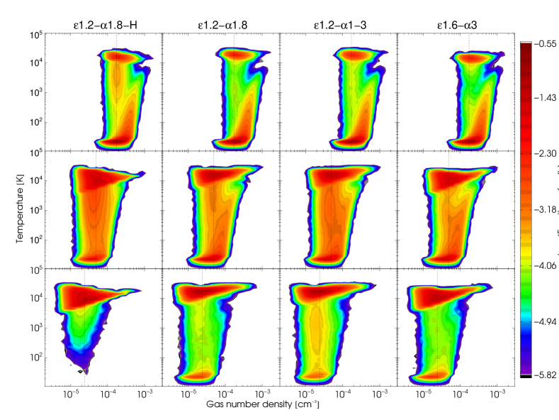
Figure 7: Contour plots of the distribution of gas temperature against proper number density for models ${\mathcal{E}}$1.2-$\alpha$1.8-H, ${\mathcal{E}}$1.2-$\alpha$1.8, ${\mathcal{E}}$1.2-$\alpha$1-3 and ${\mathcal{E}}$1.6-$\alpha$3 (from left to right). The colour scale corresponds to the percentage of cells within each contour. The rows refer to redshift $z$=14, 9 and 7 (from top to bottom). The dashed vertical lines correspond to the average density in the box.

We can also isolate the effect of the source spectrum from the volume filling factor of ionised regions by calculating the volume averaged temperature in H$\,\rm\scriptstyle II\$and He$\,\rm\scriptstyle III\$regions only, i.e. in regions with $x_{\rm HII}>x_{\rm min}$ (middle panel) and $x_{\rm HeIII}>x_{\rm min}$ (lower panel), where $x_{\min}=0.9$. We have verified that varying our choice of threshold results in similar average temperatures as long as $x_{\min}>0.1$. The gas temperature reaches its maximum value in the H$\,\rm\scriptstyle II\$and He$\,\rm\scriptstyle III\$regions at the highest redshift, when only a small percentage of cells ($<1$ per cent) in the vicinity of the first sources have been reached by ionising photons and there has been very little time for the gas to cool. As reionisation proceeds, more cells are ionised, but those that have been ionised earlier start to cool primarily by adiabatic expansion (for gas close to mean density) and Compton scattering. The net result is the average temperature in H$\,\rm\scriptstyle II\$regions decreases until $z\sim 12$ (when $\sim 5$ per cent of the cells have $x_{\rm HII}>x_{\rm min}$). At lower redshifts, an increase in the number of cells in H$\,\rm\scriptstyle II\$regions which have also experienced He$\,\rm\scriptstyle II\$photo-heating, combined with the fact that more cells are being reionised per unit time with the increasing emissivity, results in the volume averaged H$\,\rm\scriptstyle II\$region temperatures gradually increasing again toward $z=6$. Note, however, that for model ${\mathcal{E}}$1.2-$\alpha$1.8-H, where He$\,\rm\scriptstyle II\$heating is absent, the temperature starts to fall again at $z<8$ once H$\,\rm\scriptstyle I\$reionisation is complete and the ionising emissivity begins to decline.

The behaviour of the volume averaged temperature in the He$\,\rm\scriptstyle III\$regions (lower panel) is broadly similar to the case for H$\,\rm\scriptstyle II\$regions, with a high initial temperature followed by cooling. However, in this instance the temperature remains almost constant at $z<12$. Here the effect of cooling is offset by the temperature increase due to freshly ionised He$\,\rm\scriptstyle III\$regions which continue to grow at $z<6$. Finally, note that for both the H$\,\rm\scriptstyle II\$and He$\,\rm\scriptstyle III\$regions, models ${\mathcal{E}}$1.2-$\alpha$1.8 and ${\mathcal{E}}$1.2-$\alpha$1-3 always exhibit higher temperatures compared to the other models because of the energy input from hard photons during He$\,\rm\scriptstyle II\$photo-heating. This is of particular relevance when comparisons with observations are made, and will be further discussed in Section 6.

5.3 The IGM temperature-density relation

The temperatures in the simulations are examined in more detail in Figure 7, which displays the distribution of the gas temperature versus the proper number density for ${\mathcal{E}}$1.2-$\alpha$1.8-H, ${\mathcal{E}}$1.2-$\alpha$1.8, ${\mathcal{E}}$1.2-$\alpha$1-3 and ${\mathcal{E}}$1.6-$\alpha$3 (from left to right). From top to bottom, each row displays the temperature-density plane at redshift $z$=14, 9 and 7. For reference, the volume averaged temperatures at $z$=14, 9 and 7 for all models are given in Table 2. All cases show common features. While initially most of the neutral gas lies along a cold ($\sim$ 25 K) isothermal locus, as reionisation proceeds more cells are photo-heated into a second, multi-valued grouping at higher temperature. At $z=14$, a plume of hotter gas extending out to $T\simeq 10^{3}\rm\,K$ from the cold grouping toward higher densities is clearly apparent; this is due to shocked heated gas in the hydrodynamical simulation. Towards the end of reionisation, the vast majority of cells have reached their maximum temperature, which depends primarily on the ionising spectrum adopted. The fact that ionisation proceeds at a faster pace in model ${\mathcal{E}}$1.2-$\alpha$1.8-H is reflected by the temperature behaviour: while at $z=7$ almost all the cells in case ${\mathcal{E}}$1.2-$\alpha$1.8-H have been reached by ionising photons and thus heated up, in the other three models many cells are still cold and neutral.

There is also a significant amount of scatter in the temperature at fixed density at all redshifts. This scatter arises from the different reionisation history of each cell in the simulation (i.e. inhomogeneous reionisation) as well as the fact that we do not use monochromatic photons, but rather a spectral energy distribution which can also be hardened by spectral filtering (Abel & Haehnelt 1999). This differs significantly from the tight, power-law temperature-density relation expected in the optically thin case following reionisation (Hui & Gnedin 1997).

There are also some small quantitative differences in the slope and amplitude of the temperature-density relation $T=T_{0}\Delta^{\gamma-1}$, which are summarised in Table 3. It has been noted both observationally (Becker et al. 2007) and theoretically (Bolton et al. 2004; Tittley & Meiksin 2007; Trac et al. 2008; Furlanetto & Oh 2009) that the temperature-density relation may be multiple valued and inverted following H$\,\rm\scriptstyle I\$reionisation. This occurs because voids tend to be reionised last and have therefore had less time to cool. The theoretical study of Trac et al. (2008) in particular found $\gamma-1\sim-0.2$ at the end of reionisation. These authors used a larger simulation volume ($100h^{-1}$ Mpc) compared to this work, but found the strong correlation between the density field and redshift of reionisation in these models extends down to scales of $1h^{-1}$ Mpc. We find the temperature-density relation is indeed very mildly inverted ($\gamma-1\sim-0.05$) for ${\mathcal{E}}$1.2-$\alpha$1.8-H at $z=14$, but it remains close to isothermal for all other models at all redshifts. The origin of the diffferences between Trac et al. (2008) and this work are not clear. One possibility, however, is that Trac et al. (2008) used a rather different prescription for the source emissivity based on the star formation implementation of Trac & Cen (2007). The ionising photon production rate in this model is not calibrated to match constraints from the Ly$\alpha$ forest data, and it therefore rises continuously toward lower redshift. This means that the latter stages of reionisation occur more rapidly in their simulations compared to our model. A more rapid end to reionisation could potentially explain the more strongly inverted temperature-density relation Trac et al. (2008) find; proportionally more of the underdense gas will have been reionised and reheated close to the end of reionisation.

Table 3: The temperature-density relation of the ionised IGM in our simulations. The columns indicate, from left to right, the name of the model, the redshift $z$, and the best fit power-law parameters for the power-law temperature-density relation $T=T_{0}\Delta^{\gamma-1}$. Here $T_{0}$ and $\gamma-1$ are calculated only in cells with $x_{\rm HII}>0.99$ (columns 3 and 5) and $x_{\rm HeIII}>0.99$ (columns 4 and 6). See text for further details.

Model	$z$	$T_{0}$ [K]		$\gamma$-1
		$x_{\rm HII}>0.99$	$x_{\rm HeIII}>0.99$	$x_{\rm HII}>0.99$	$x_{\rm HeIII}>0.99$
	14	16744	–	-0.0404	–
	9	10525	–	0.0116	–
${\mathcal{E}}$1.2-$\alpha$1.8-H	7	9293	–	0.0313	–
	6	8648	–	0.0419	–
	14	19705	17027	-0.0153	0.0101
	9	14272	11735	0.0381	0.0567
${\mathcal{E}}$1.2-$\alpha$1.8	7	15823	14080	0.0367	0.0559
	6	15927	15008	0.0341	0.0357
	14	18885	16743	-0.0055	0.0123
	9	14145	11796	0.0385	0.0641
${\mathcal{E}}$1.2-$\alpha$1-3	7	15826	12624	0.0370	0.0678
	6	16236	14970	0.0351	0.0455
	14	14285	13828	0.0014	0.0179
	9	10058	10753	0.0434	0.0438
${\mathcal{E}}$1.6-$\alpha$3	7	9922	11511	0.0554	0.0483
	6	9725	13386	0.0594	0.0465
	14	14035	13779	0.0045	0.0169
	9	10049	11005	0.0425	0.0412
${\mathcal{E}}$1.2-$\alpha$3	7	10649	11852	0.0437	0.0424
	6	10468	13038	0.0453	0.0544

6 Implications for reionisation sources

In this section we now consider the implications our empirically motivated simulations for reionisation by comparing them to observational constraints on the IGM temperature at mean density, the volume averaged neutral hydrogen fraction and recent estimates of the ionising emissivity from measurements of the UV galaxy luminosity function at $4<z<8$.

6.1 The thermal state of the IGM at $z\simeq 5-6$

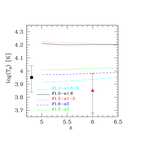
Figure 8: The IGM temperature at mean density, $T_{0}$, at different redshifts (see Table 3). The filled symbols refers to the values measured by Becker et al. (2011, black square) and Bolton et al. (2012, red triangle). The curves refer instead to the simulated results from models ${\mathcal{E}}$1.2-$\alpha$1.8-H (long dashed cyan), ${\mathcal{E}}$1.2-$\alpha$1.8 (solid black), ${\mathcal{E}}$1.2-$\alpha$1-3 (dotted red), ${\mathcal{E}}$1.6-$\alpha$3 (dashed blue) and ${\mathcal{E}}$1.2-$\alpha$3 (dotted-dashed green).

We first compare our simulations to recent measurements of the IGM temperature in Figure 8 (see also Raskutti et al. 2012). Becker et al. (2011) recently presented constraints on the thermal state of the IGM based on Ly$\alpha$ forest observations in the redshift range $2.0<z<4.8$. Their temperature measurement at $z=4.8$ is reported as $T_{0}=8930\pm 2020$ K ($2\sigma$ errors) assuming an isothermal temperature-density relation ($\gamma=1$). This constraint is shown by the black square in Figure 8. At higher redshift, $z\sim 6$, Bolton et al. (2012) have measured the temperature of the IGM within $\sim 5$ proper Mpc of seven quasars using the Doppler widths of Ly$\alpha$ absorption lines. They report a line-of-sight averaged temperature at the mean density of $T_{0}\sim 16200$ K. Note, however, this constraint is complicated by the fact that these quasars also reionise the He$\,\rm\scriptstyle II\$in their vicinity due to their hard ionising spectra. Bolton et al. (2012) therefore also provided an estimate for the temperature after subtracting the expected heating from the local reionisation of He$\,\rm\scriptstyle II\$by the quasars, $T_{0}\sim 7100\rm\,K$, assuming a quasar EUV spectral index of $\alpha=1.5$. This latter estimate is displayed in Figure 8 as the red triangle with 95 per cent confidence error bars. Lastly, note that this constraint is dependent on the uncertain amount of He$\,\rm\scriptstyle II\$heating expected from the quasars; assuming a harder (softer) EUV spectral index for the quasars would lower (raise) this temperature constraint by several thousand degrees.

Keeping this in mind, the curves in Figure 8 display the temperature at mean density, $T_{0}$, calculated in cells with $x_{\rm HII}>0.99$ (see Table 3) in models ${\mathcal{E}}$1.2-$\alpha$1.8-H (long dashed cyan), ${\mathcal{E}}$1.2-$\alpha$1.8 (solid black), ${\mathcal{E}}$1.2-$\alpha$1-3 (dotted red), ${\mathcal{E}}$1.6-$\alpha$3 (dashed blue) and ${\mathcal{E}}$1.2-$\alpha$3 (dotted-dashed green). We estimate the temperature from the simulations in this manner to ensure any neutral gas which has yet to be ionised is excluded; the temperature measurements from the Ly$\alpha$ absorption measurements only probe highly ionised hydrogen. The simulations which have a soft ($\alpha=3$) EUV spectral index (${\mathcal{E}}$1.2-$\alpha$3 and ${\mathcal{E}}$1.6-$\alpha$3) as well as the model which excludes helium (${\mathcal{E}}$1.2-$\alpha$1.8-H) are similar or slightly greater than (within $\sim 0.02$ dex of the 95 per cent confidence interval) the measurement obtained by Bolton et al. (2012) at $z\sim 6$. In contrast, the two models with harder spectra (${\mathcal{E}}$1.2-$\alpha$1.8 and ${\mathcal{E}}$1.2-$\alpha$1-3) exhibit significantly higher temperatures due to additional He$\,\rm\scriptstyle II\$photo-heating. Similarly, the Becker et al. (2011) temperature measurement at $z=4.8$ is also much lower than the predicted simulation temperatures at $z=5$ for the harder ionising spectra. Note that the agreement would be even worse if the heating contribution from X-rays were included in the simulations.

These results are thus consistent with a predominance of sources with relatively soft ($\alpha\geq 3$) ionising spectra during hydrogen reionisation, and also with an epoch of He$\,\rm\scriptstyle II\$reionisation (most likely driven by quasars) which was not fully underway until lower redshift (e.g. McQuinn et al. 2009). We therefore conclude that if a population of sources with rather hard spectra, such as mini-quasars (Madau et al. 2004) or population-III stars (Bromm et al. 2001b) were responsible for reionising hydrogen, their contribution must be either (i) sub-dominant at all redshifts or (ii) confined predominantly at early times ($z\geq 9$), such that there has been sufficient time for the IGM temperature to cool and doubly ionised helium to recombine by $z\simeq 6$. This is not surprising as population-III stars are believed to be present at $z<9$, but, compared to population-II stars, in negligible numbers (see e.g. Tornatore et al. 2007; Maio et al. 2010). Becker et al. (2012) have also recently pointed out that relative metal abundances in the IGM suggest population-II stars produced the bulk of hydrogen ionising photons during reionisation. Similarly, although mini-quasars have been investigated by a number of authors as possible sources of ionising photons, the general agreement is that their contribution is not dominant (see e.g. Madau et al. 2004; Miralda-Escudé et al. 2000). In addition, a model in which reionisation were dominated by mini-quasars would most likely overpredict also the observed soft X-ray background Salvaterra et al. (2005).

6.2 Ionising photon production

We next compare the ionising emissivity used in our simulations to observational estimates based on recent measurements of the galaxy luminosity function at $4<z<8$. For this purpose, we compute the ionising emissivity from galaxies using the recent fit to the redshift evolution of the galaxy luminosity function presented by Bouwens et al. (2011). We assume a spectral energy distribution $\epsilon_{\nu}\propto\nu^{0}$ for $912{\rm\AA}<\lambda<3000\rm\AA$ and $\epsilon_{\nu}\propto\nu^{-3}$ (i.e. $\alpha=3$) for $\lambda<912\rm\AA$, with an additional factor of six break at the Lyman limit (e.g. Leitherer et al. 1999; Madau et al. 1999). In addition, we adopt two different redshift evolutions for the faint-end slope: the Bouwens et al. (2011) best fit $\alpha_{\rm LF}=-1.84-0.05(z-6)$, and a steeper faint end slope of $\alpha_{\rm LF}=-1.9-0.1(z-6)$. These choices are intented to represent the considerable observational uncertainty in the faint-end slope.

The resulting emissivities are displayed as the hatched regions in Figure 9, with the results from the two different faint end slope evolutions shown in each panel. The cyan and orange hatching assume ionising photon escape fractions of $f_{\rm esc}=0.2$ and $f_{\rm esc}=0.5$, while the lower and upper limits to the hatching correspond to the emissivity obtained by integrating the Bouwens et al. (2011) luminosity function fit to a lower magnitude limit of $M_{\rm UV}=-18$ and $M_{\rm UV}=-10$, respectively. These limits roughly correspond to the magnitude limit of the observational data and the expected magnitude of a galaxy in a halo with virial temperature $2\times 10^{4}\rm\,K$ (Trenti et al. 2010), respectively. These are compared to the emissivities used in models ${\mathcal{E}}$1.2-$\alpha$3 (solid curve) and ${\mathcal{E}}$1.6-$\alpha$3 (dashed curve). Observational constraints on the emissivity at $z\leq 6$ (red circles with error bars) derived from measurements of the photo-ionisation rate from the Ly$\alpha$ forest (Wyithe & Bolton 2011) and mean free path (Songaila & Cowie 2010) are displayed as red circles with error bars. Note again, that the models are by construction chosen to match these constraints closely.

In order to match the emissivity in model ${\mathcal{E}}$1.2-$\alpha$3 up to $z=8$, an extrapolation of the faint end of the luminosity function to $M_{\rm UV}=-10$, a high escape fraction $f_{\rm esc}=0.5$ and a slightly steeper faint-end slope than the best fit of Bouwens et al. (2011) are required. Faint (and currently undetected) galaxies are thus required to reproduce the ionising emissivity in our simulations. Recent theoretical studies indicate the faint end slope may indeed steepen at $z>6$ (Trenti et al. 2010; Jaacks et al. 2012). A rather high Lyman continnum escape fraction is also required from these faint galaxies. Although impossible to measure directly at $z>6$, recent observations indicate the escape fraction at $z\sim 3$ is larger than at later times (e.g. Siana et al. 2010). In addition, Rauch et al. (2011) have recently presented observations of a morphologically disturbed, faint Ly$\alpha$ emitting galaxy at $z=3.44$ which are consistent with a Lyman continuum escape fraction of 50 per cent. These authors note that such faint, interacting galaxies may be more common at higher redshift, where the increasing importance of gravitational interactions and mergers could provide a plausible mechanism for such high escape fractions.

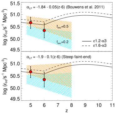
Figure 9: The ionising emissivity in models ${\mathcal{E}}1.2-\alpha 3$ (solid curve) and ${\mathcal{E}}1.6-\alpha 3$ (dashed curve) compared to observational constraints based on Ly$\alpha$ forest data at $z\leq 6$ (red circles) and estimates of the emissivity from recent constraints on the luminosity function of high redshift Lyman break galaxies by Bouwens et al. (2011) (hatched regions). Upper panel: Comparison to the emissivity derived from the best fit redshift evolution of the luminosity function at $4<z<8$ presented by Bouwens et al. (2011) (see text for details) with a faint end slope $\alpha_{\rm F}=-1.84-0.05(z-6)$. The cyan and orange hatching assume escape fractions of $f_{\rm esc}=0.2$ and $f_{\rm esc}=0.5$, respectively, while the range of the hatched regions corresponds to the emissivity obtained by integrating the luminosity function to a lower magnitude limit of $M_{\rm lim}=-10$ and $M_{\rm lim}=-18$ (upper and lower limit to hatching, respectively). Lower panel: As for upper panel, but now assuming a steeper faint end slope for the luminosity function, $\alpha_{\rm LF}=-1.9-0.1(z-6)$.

Finally, the emissivity evolution in our simulations is such that a halo with a baryon mass $M_{\rm b}=10^{8}$ M_⊙ at $z=14$ produces $\sim 5\times 10^{52}$ phot s^-1 and $\sim 10^{50}$ phot s^-1 at $z=6$. For comparison, the number of ionising photons emitted by a halo with baryon mass $M_{\rm b}=M_{\rm tot}(\Omega_{\rm b}/\Omega_{\rm m})$ can be written as (see Iliev et al. 2006):

$$\dot{N} = \frac{f_{\star}f_{\rm esc}N_{\rm phot}M_{\rm b}}{m_{\rm p}\Delta t}$$

$$\simeq 5\times 10^{52}{\,\rm phot\;s^{-1}}$$

$$\times \left(\frac{f_{\star}}{0.05}\right)\left(\frac{f_{\rm esc}}{0.5}\right)\left(\frac{N_{\rm phot}}{5\times 10^{3}}\right)\left(\frac{M_{\rm b}}{10^{8}\;{\rm M_{\odot}}}\right)\left(\frac{10^{7}\;{\rm yr}}{\Delta t}\right),$$

where $f_{\star}$ is the fraction of baryons which are converted into stars, $f_{\rm esc}$ is the escape fraction of ionising photons, $N_{\rm phot}$ is the number of ionising photons per stellar baryon, $m_{\rm p}$ is the proton mass and $\Delta t$ is the time between two snapshots of the hydrodynamical simulation. Typically, $N_{\rm phot}=5\times 10^{3}$ and $1\times 10^{4}$ for population-II stars with a Salpeter IMF and a top-heavy IMF, respectively (e.g. Iliev et al. 2006). The requirement for a large escape fraction ($f_{\rm esc}\sim 0.5$) may be therefore relaxed somewhat if the efficiency of ionising photon production increases toward higher redshift or a top-heavy IMF is invoked (see e.g. Bromm et al. 2001a; Schneider et al. 2002). However, as noted in the previous section, the IGM temperature measurements appear to rule out significant reionisation by metal-free stellar populations, at least at $z<9$. However, as there are a variety of possible parameter combinations which could satisfy the emissivity required, it is not possible to set a stringent constraint on the individual parameters in Eq. (6.2).

6.3 The volume averaged H$\,\rm\scriptstyle I\$fraction

Lastly, we compare our simulations to constraints on the volume averaged H$\,\rm\scriptstyle I\$fraction, $x_{\rm HI}$, in the IGM at $z\geq 6$. As discussed earlier, the presently available observational data remain inconclusive with regard to the redshift evolution of $x_{\rm HI}$. This is largely because almost all the methods used to derive $x_{\rm HI}$ are somewhat model dependent and/or are limited by the available data. For example, at $z=5.5$, studies of the transmitted flux in the Ly$\alpha$ forest indicate $x_{\rm HI}\sim 10^{-4}$ (Fan et al., 2006; Becker et al., 2007; Bolton & Haehnelt, 2007) in the regions where Ly$\alpha$ transmission is detected. However, Mesinger (2010) has noted that the relatively small number of quasar sight-lines which have been analysed, combined with the fact that quasars sit in highly biased regions, does not preclude an IGM which is still a few per cent neutral by volume at $z=5$–$6$; isolated patches of neutral hydrogen may still lurk undetected in the diffuse IGM at these redshifts due to the inhomogeneous nature of reionisation (see also Lidz et al. 2007). Indeed, taking an (almost) model independent approach, McGreer et al. (2011) calculated a conservative upper limit of $x_{\rm HI}\lower 2.15277pt\hbox{$\;\buildrel<\over{\sim}\;$}0.9$ from Ly$\alpha$ forest data at $z\sim 6.1$, although a subsample of two deep spectra provided a more stringent constraint of $x_{\rm HI}\lower 2.15277pt\hbox{$\;\buildrel<\over{\sim}\;$}0.5$.

Alternative analyses of higher redshift quasar spectra also provide variable estimates. An analysis of a putative IGM damping wing in a quasar near-zone at $z=6.28$ by Mesinger & Haiman (2004) yields $x_{\rm HI}\lower 2.15277pt\hbox{$\;\buildrel>\over{\sim}\;$}0.2$. In contrast, Maselli et al. (2007) find that the sizes of quasar near-zones are consistent with an IGM which is mostly ionized at $z\simeq 6$, with $x_{\rm HI}\lower 2.15277pt\hbox{$\;\buildrel<\over{\sim}\;$}0.06$. More recently, an analysis of the near-zone in the spectrum of the highest redshift quasar yet detected was found to be consistent with $x_{\rm HI}\lower 2.15277pt\hbox{$\;\buildrel>\over{\sim}\;$}0.1$ at $z=7.085$ (Mortlock et al., 2011; Bolton et al., 2011). However, all of these observations probe only the neutral fraction in the vicinity of these quasars, so the interpretation of these measurements with respect to the IGM as a whole is again hampered by the inhomogeneous nature of reionisation (Mesinger & Furlanetto 2008). Lastly, recent measurements of a rapid decline in the Ly$\alpha$ emitter/Lyman break galaxy fraction indicate the neutral fraction may be as high as $x_{\rm HI}\sim 0.5$ at $z\sim 7$ (Schenker et al. 2012; Pentericci et al. 2011; Ono et al. 2011). On the other hand, the effect of patchy reionisation and galactic outflows on reionisation also complicate the use of Ly$\alpha$ emitting galaxies as a probe of the volume averaged neutral fraction (e.g. Dijkstra et al. 2011).

In Figure 10 we present a comparison between the volume averaged neutral fraction predicted by our simulations and a selection of these measurements. There are two important points to note here. Firstly, all our simulations lie within the (admittedly large) region between the lower and upper limits at $z\simeq 6$. However, the Mortlock et al. (2011) measurement appears to exclude all the models with the exception of ${\mathcal{E}}$1.2-$\alpha$3; the neutral fraction in all the other cases is too low and as a consequence the emissivity is too high. Reconciling these models with the Mortlock et al. (2011) neutral fraction at $z\sim 7.1$ would therefore require a lower ionising emissivity which then must remain constant or even increase weakly toward lower redshift to simultaneously match the $z=6$ photo-ionisation rate measurements. On the other hand, Bolton et al. (2011) note that uncertainties in the abundance of high column density systems and the spectral shape of the quasar ionising radiation could weaken the upper limit on $x_{\rm HI}$, so the significance of this difference should be treated cautiously.

The second (related) point is that all four models which include helium predict a neutral fraction at $z=6$ between $1$–$6$ per cent, which lies 1–2 orders of magnitude above the constraints from the Ly$\alpha$ forest opacity. This is in stark contrast to the conventional interpretation that the IGM is highly ionised, $x_{\rm HI}\sim 10^{-4}$, by $z=6$, although this scenario is consistent with the conservative estimates of McGreer et al. (2011). This result is perhaps not too surprising; numerical models which predict a highly ionised IGM at $z=6$ typically overpredict the photo-ionisation rate or ionising intensity by a factor of two or more (e.g. Iliev et al. 2008; Finlator et al. 2009; Aubert & Teyssier 2010). This implies that when we deliberately match the emissivity in our simulations at $z=6$ to the Ly$\alpha$ forest data, the IGM is required to have an appreciable neutral fraction at $z\sim 6$. A more highly ionised IGM by $z=6$ may be obtained by adopting an ionising emissivity which increases more rapidly than we already assume at $z>6$, but this would still come at the expense of not satisfying the $z\sim 7$ neutral fraction constraint.

An important caveat, however, is that most reionisation models (including this work) do not correctly resolve Lyman limit systems (although see Kohler & Gnedin 2007; McQuinn et al. 2011). Lyman limit systems (LLSs) are expected to regulate the mean free path of ionising photons once the sizes of ionised bubbles exceed the typical separation between these optically thick systems (Gnedin & Fan 2006; Furlanetto & Mesinger 2009). Since the H$\,\rm\scriptstyle I\$photo-ionisation rate is proportional to the emissivity and the mean free path, $\Gamma_{\rm HI}\propto\epsilon_{\rm HI}\lambda_{\rm HI}$, correctly modelling LLSs is a crucial ingredient for simulating the latter stages of reionisation. Although our simulations match the observational measurements of $\Gamma_{\rm HI}$ by design, the mean free path within the simulations is not set by LLSs, but rather the remaining patches of neutral gas in the IGM which are furthest from the ionising sources (in the case of ${\mathcal{E}}$1.2-$\alpha$3, this is 6 per cent of the IGM by volume at $z=6$). A mean free path at $z=6$ which is instead set by LLSs might allow for an emissivity which is consistent with the observed constraints on $\Gamma_{\rm HI}$, but at the same time have a lower volume averaged neutral fraction due to the smaller volume filling factor of these dense optically thick systems.

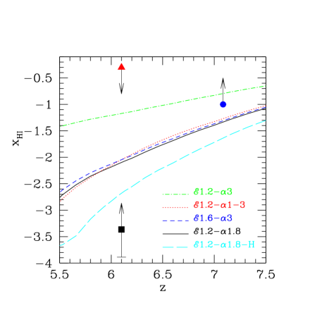
Figure 10: The volume averaged H$\,\rm\scriptstyle I\$fraction and its evolution with redshift. The filled symbols refer to the observational measurements by Fan et al. (2006, black square), McGreer et al. (2011, red triangle) and Mortlock et al. (2011, blue circle, see text for further details). The curves display the results of our radiative transfer simulations: ${\mathcal{E}}$1.2-$\alpha$1.8-H (long dashed cyan), ${\mathcal{E}}$1.2-$\alpha$1.8 (solid black), ${\mathcal{E}}$1.2-$\alpha$1-3 (dotted red), ${\mathcal{E}}$1.6-$\alpha$3 (dashed blue) and ${\mathcal{E}}$1.2-$\alpha$3 (dotted-dashed green).

Note again, however, that the issue of how one could then reconcile the large volume averaged neutral fraction of $x_{\rm HI}>0.1$ at $z=7.1$ with (i) a low neutral fraction of $x_{\rm HI}\sim 10^{-4}$ at $z=6$ and (ii) an emissivity at $z=6$ equivalent to $\sim 1$–$3$ ionising photons emitted per hydrogen atom over a Hubble time remains. Since the emissivity must increase at $z>6$ for reionisation to complete by $z=6$ (Bolton & Haehnelt 2007), either the IGM is more highly ionised at $z\sim 7$ than recent observations suggest, or the IGM is still a few per cent neutral by volume at $z=6$ (Mesinger 2010).

7 Summary and conclusions

In this work we have investigated the impact of helium on hydrogen reionisation using three dimensional, multi-frequency RT simulations. We performed five simulations using different models for the amplitude and spectral shape of the ionising emissivity during reionisation. By design, all our models are consistent with measurements of the Thomson scattering optical depth and the metagalactic hydrogen photo-ionisation rate at $z\sim 6$. This empirical approach enables us to explore the consequences of satisfying these observational constraints for reionisation. The main outcomes of this study may be summarised as follows.

• The evolution of the volume averaged H$\,\rm\scriptstyle II\$fraction, $x_{\rm HII}$, is very similar for all models with the same hydrogen ionising emissivity independent of the EUV spectral index. However, the spectral energy distribution has a strong impact on the evolution on the volume averaged He$\,\rm\scriptstyle II\$and He$\,\rm\scriptstyle III\$fractions, $x_{\rm HeII}$ and $x_{\rm HeIII}$. Models with a soft power-law EUV index, $\alpha=3$, produce a much lower $x_{\rm HeIII}$ compared to models in which harder photons are present. The inclusion of helium in the RT simulations furthermore slightly delays reionisation due to the small number of ionising photons which reionise neutral helium instead of hydrogen.
  

• The choice of EUV spectral index has a significant effect on the evolution of the volume averaged IGM temperature during reionisation. At $z\lower 2.15277pt\hbox{$\;\buildrel>\over{\sim}\;$}10$, model ${\mathcal{E}}$1.2-$\alpha$1.8-H (without helium) has a volume averaged temperature which is $\sim 10$ per cent higher than the corresponding model including helium, ${\mathcal{E}}$1.2-$\alpha$1.8, due to the slightly larger volume of the IGM which is photo-ionised by this time. However, at lower redshift the inclusion of He$\,\rm\scriptstyle II\$photo-ionisation results in a higher volume averaged temperature for ${\mathcal{E}}$1.2-$\alpha$1.8. In comparison, despite exhibiting behaviour similar to ${\mathcal{E}}$1.2-$\alpha$1.8 and ${\mathcal{E}}$1.2-$\alpha$1-3 for the evolution of the H$\,\rm\scriptstyle II\$filling factor, the softer ionising spectrum used in ${\mathcal{E}}$1.6-$\alpha$3 produces volume averaged temperatures which are 20-30 per cent lower than ${\mathcal{E}}$1.2-$\alpha$1.8. This is partly because the volume filling factor of He$\,\rm\scriptstyle III\$is smaller in this model, but also because the softer ionising photons produce less photo-heating.
  

• The temperature (and ionisation fraction) distributions in the simulations exhibit a significant amount of scatter at all redshifts. This scatter arises from the different reionisation history of each cell in the simulations (i.e. inhomogeneous reionisation) as well as the fact that we do not use monochromatic photons, but rather a spectral energy distribution which can also be hardened by spectral filtering. This differs significantly from the tight, power-law temperature-density relation expected for an optically thin IGM following reionisation. We find the temperature-density relation for ionised gas is typically isothermal or mildly inverted during hydrogen reionisation.
  

• A comparison with recent estimates of the IGM temperature at $z\sim 5-6$ from Ly$\alpha$ absorption in the spectra of high redshift quasars suggests that hydrogen reionisation is mainly driven by sources with a soft spectral energy distribution, $\alpha\leq 3$. The simulations with harder spectral indices produce temperatures which are larger than the observational constraints. We conclude that population-II stellar sources are likely to provide most of the ionising photons during reionisation, and the spectral shape of the ionising background must harden at $z<6$ due to the increasing importance of quasars if He$\,\rm\scriptstyle II\$reionisation is to complete by $z\simeq 3$. If sources with rather hard spectra, such as mini-quasars or population-III stars were responsible for reionising hydrogen, their contribution must be either small or confined to $z\geq 9$ to give sufficient time for the IGM temperature to cool and for doubly ionised helium to recombine by $z\simeq 6$.
  

• In order to reproduce the ionising emissivity in our simulations at $z>6$, we find that the best fit to the evolution of the galaxy luminosity function presented by Bouwens et al. (2011) at $4<z<8$ requires extrapolation to faint UV magnitudes ($M_{\rm UV}=-10$), as well as a steepening faint end slope $\alpha_{\rm LF}\leq-2$ and a high Lyman continuum escape fraction $f_{\rm esc}=0.5$. Faint, low mass galaxies are therefore necessary for providing the required number of photons during reionisation, in agreement with several other complementary studies.
  

• There is some tension between the empirically motivated ionising emissivity used in our simulations and recent observational constraints on the IGM neutral fraction which indicate that $x_{\rm HI}>0.1$ at $z\sim 7.1$. The ionising emissivity inferred from the Ly$\alpha$ forest at $z=6$ is equivalent to only $1$–$3$ ionising photons emitted per hydrogen atom over a Hubble time, implying reionisation is extended and that the emissivity must increase at $z>6$ if reionisation is to complete by $z=6$ (Miralda-Escudé 2003; Bolton & Haehnelt 2007). However, an increasing emissivity at $z>6$ is inconsistent with a large neutral fraction at $z\sim 7$ in our simulations unless the observations are overestimates or the IGM remains a few per cent neutral by volume at $z=6$ (see e.g Mesinger 2010).

Our results highlight the importance of reproducing post-reionisation constraints such as the IGM temperature and background photo-ionisation rate for constraining reionisation models. While these simulations were designed mainly to investigate the impact of helium on hydrogen reionisation and the sources of ionising photons at high redshift, the volume used is too small to allow a more detailed discussion on helium reionisation (which is thought to be driven by quasars and to be complete at $z\sim 2.5-3$) and a more accurate comparison with observational constraints at $z<6$. We will postpone this further analysis to a future work, together with a more thorough investigation of the impact of unresolved small scale high density peaks. The latter will be particularly important for regulating the tail-end of the reionisation process and for setting the thermal state of the IGM by absorbing photons close to the H$\,\rm\scriptstyle I\$and He$\,\rm\scriptstyle II\$ionisation edges. Including these effects in numerical models is therefore necessary for refining the comparison of simulations with observations at $z<6$.

Appendix A Convergence tests

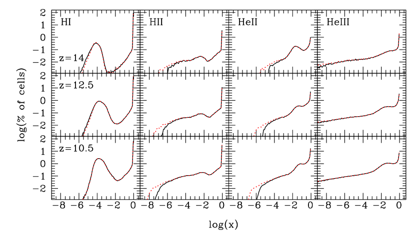
Figure 11: The percentage of cells in the radiative transfer simulations as a function of H$\,\rm\scriptstyle I$, H$\,\rm\scriptstyle II$, He$\,\rm\scriptstyle II$ and He$\,\rm\scriptstyle III$ fractions (from left to right) at $z$=14 (upper row), 12.5 (middle row) and 10.5 (lower row). The curves in each panel correspond to model ${\mathcal{E}}$1.2-$\alpha$1.8 (solid black lines) and the same model run with 10 times more photon packets (red dotted).

As discussed in Section 3.2, depending on the redshift and number of sources, we emit $10^{5}-10^{6}$ photon packets per source at each $t_{rt,i}$, corresponding to a total of $\sim 5\times 10^{7}-10^{10}$ photon packets. While it is computationally too expensive to run a full simulation with an order of magnitude more photon packets, we have run tests on single snapshots and on a limited number of consecutive snapshots at high redshift. In Figures 11 and 12 the distribution of different species and gas temperature, respectively, is shown for run ${\mathcal{E}}$1.2-$\alpha$1.8 (black solid lines) and for the same simulation with 10 times more photon packets (red dotted). The results are shown down to the lowest redshift reached by the higher resolution simulation, i.e. $z=10.5$, which is obtained using 12 snapshots of the hydrodynamic simulation. It is evident that an excellent convergence has been reached both for the H and He species and the gas temperature, with the exception of cells with $x_{\rm HII}<10^{-6}$ and $x_{\rm HeII}<10^{-4}$. Tests using only one snapshot at lower redshifts (i.e. following the radiative transfer starting from a non neutral configuration) show a similar convergence, but they do not account for differences between the two runs which might have accumulated if the full reionisation history were followed. The above Figures though demonstrate that such differences are negligible.

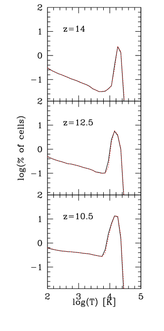
Figure 12: The percentage of cells in the radiative transfer simulations as a function of the gas temperature $T$ at $z$=14 (upper row), 12.5 (middle row) and 10.5 (lower row). The curves in each panel correspond to model ${\mathcal{E}}$1.2-$\alpha$1.8 (solid black lines) and the same model run with 10 times more photon packets (red dotted).

References

- Abel & Haehnelt (1999) Abel, T. & Haehnelt, M. G. 1999, ApJ, 520, L13
- Aubert & Teyssier (2010) Aubert, D. & Teyssier, R. 2010, ApJ, 724, 244
- Baek et al. (2010) Baek, S., Semelin, B., Di Matteo, P., Revaz, Y., & Combes, F. 2010, A&A, 523, A4
- Becker et al. (2011) Becker, G. D., Bolton, J. S., Haehnelt, M. G., & Sargent, W. L. W. 2011, MNRAS, 410, 1096
- Becker et al. (2007) Becker, G. D., Rauch, M., & Sargent, W. L. W. 2007, ApJ, 662, 72
- Becker et al. (2012) Becker, G. D., Sargent, W. L. W., Rauch, M., & Carswell, R. F. 2012, ApJ, 744, 91
- Becker et al. (2001) Becker, R. H., Fan, X., White, R. L., Strauss, M. A., Narayanan, V. K., Lupton, R. H., Gunn, J. E., Annis, J., Bahcall, N. A., Brinkmann, J., Connolly, A. J., Csabai, I., Czarapata, P. C., Doi, M., Heckman, T. M., Hennessy, G. S., Ivezić, Ž., Knapp, G. R., Lamb, D. Q., McKay, T. A., Munn, J. A., Nash, T., Nichol, R., Pier, J. R., Richards, G. T., Schneider, D. P., Stoughton, C., Szalay, A. S., Thakar, A. R., & York, D. G. 2001, AJ, 122, 2850
- Bolton et al. (2004) Bolton, J., Meiksin, A., & White, M. 2004, MNRAS, 348, L43
- Bolton et al. (2012) Bolton, J. S., Becker, G. D., Raskutti, S., Wyithe, J. S. B., Haehnelt, M. G., & Sargent, W. L. W. 2012, MNRAS, 419, 2880
- Bolton & Haehnelt (2007) Bolton, J. S. & Haehnelt, M. G. 2007, MNRAS, 382, 325
- Bolton et al. (2011) Bolton, J. S., Haehnelt, M. G., Warren, S. J., Hewett, P. C., Mortlock, D. J., Venemans, B. P., McMahon, R. G., & Simpson, C. 2011, MNRAS, 416, L70
- Bouwens et al. (2011) Bouwens, R. J., Illingworth, G. D., Oesch, P. A., Trenti, M., Labbe, I., Franx, M., Stiavelli, M., Carollo, C. M., van Dokkum, P., & Magee, D. 2011, ArXiv e-prints
- Bromm et al. (2001a) Bromm, V., Ferrara, A., Coppi, P. S., & Larson, R. B. 2001a, MNRAS, 328, 969
- Bromm et al. (2001b) Bromm, V., Kudritzki, R. P., & Loeb, A. 2001b, ApJ, 552, 464
- Calverley et al. (2011) Calverley, A. P., Becker, G. D., Haehnelt, M. G., & Bolton, J. S. 2011, MNRAS, 412, 2543
- Cantalupo & Porciani (2011) Cantalupo, S. & Porciani, C. 2011, MNRAS, 411, 1678
- Choudhury & Ferrara (2006) Choudhury, T. R. & Ferrara, A. 2006, MNRAS, 371, L55
- Ciardi et al. (2001) Ciardi, B., Ferrara, A., Marri, S., & Raimondo, G. 2001, MNRAS, 324, 381
- Ciardi et al. (2003) Ciardi, B., Ferrara, A., & White, S. D. M. 2003, MNRAS, 344, L7
- Dijkstra et al. (2011) Dijkstra, M., Mesinger, A., & Wyithe, J. S. B. 2011, MNRAS, 414, 2139
- Fan et al. (2006) Fan, X., Strauss, M. A., Richards, G. T., Hennawi, J. F., Becker, R. H., White, R. L., Diamond-Stanic, A. M., Donley, J. L., Jiang, L., Kim, J. S., Vestergaard, M., Young, J. E., Gunn, J. E., Lupton, R. H., Knapp, G. R., Schneider, D. P., Brandt, W. N., Bahcall, N. A., & Barentine, J. C. 2006, AJ, 131, 1203
- Finlator et al. (2009) Finlator, K., Özel, F., & Davé, R. 2009, MNRAS, 393, 1090
- Friedrich et al. (2012) Friedrich, M. M., Mellema, G., Iliev, I. T., & Shapiro, P. R. 2012, MNRAS, 2385
- Furlanetto & Mesinger (2009) Furlanetto, S. R. & Mesinger, A. 2009, MNRAS, 394, 1667
- Furlanetto & Oh (2009) Furlanetto, S. R. & Oh, S. P. 2009, ApJ, 701, 94
- Gnedin & Fan (2006) Gnedin, N. Y. & Fan, X. 2006, ApJ, 648, 1
- Gunn & Peterson (1965) Gunn, J. E. & Peterson, B. A. 1965, ApJ, 142, 1633
- Haardt & Madau (2001) Haardt, F. & Madau, P. 2001, in Clusters of Galaxies and the High Redshift Universe Observed in X-rays, ed. D. M. Neumann & J. T. V. Tran
- Haardt & Madau (2012) Haardt, F. & Madau, P. 2012, ApJ, 746, 125
- Hockney & Eastwood (1988) Hockney, R. W. & Eastwood, J. W. 1988, Computer Simulation using Particles, Hilger, Bristol
- Hui & Gnedin (1997) Hui, L. & Gnedin, N. Y. 1997, MNRAS, 292, 27
- Iliev et al. (2006) Iliev, I. T., Mellema, G., Pen, U., Merz, H., Shapiro, P. R., & Alvarez, M. A. 2006, MNRAS, 369, 1625
- Iliev et al. (2007) Iliev, I. T., Mellema, G., Shapiro, P. R., & Pen, U. 2007, MNRAS, 376, 534
- Iliev et al. (2008) Iliev, I. T., Shapiro, P. R., McDonald, P., Mellema, G., & Pen, U. 2008, MNRAS, 391, 63
- Jaacks et al. (2012) Jaacks, J., Choi, J.-H., Nagamine, K., Thompson, R., & Varghese, S. 2012, MNRAS, 420, 1606
- Kohler & Gnedin (2007) Kohler, K. & Gnedin, N. Y. 2007, ApJ, 655, 685
- Komatsu et al. (2011) Komatsu, E., Smith, K. M., Dunkley, J., Bennett, C. L., Gold, B., Hinshaw, G., Jarosik, N., Larson, D., Nolta, M. R., Page, L., Spergel, D. N., Halpern, M., Hill, R. S., Kogut, A., Limon, M., Meyer, S. S., Odegard, N., Tucker, G. S., Weiland, J. L., Wollack, E., & Wright, E. L. 2011, ApJS, 192, 18
- Leitherer et al. (1999) Leitherer, C., Schaerer, D., Goldader, J. D., Delgado, R. M. G., Robert, C., Kune, D. F., de Mello, D. F., Devost, D., & Heckman, T. M. 1999, ApJS, 123, 3
- Lidz et al. (2007) Lidz, A., McQuinn, M., Zaldarriaga, M., Hernquist, L., & Dutta, S. 2007, ApJ, 670, 39
- Madau et al. (1999) Madau, P., Haardt, F., & Rees, M. J. 1999, ApJ, 514, 648
- Madau et al. (2004) Madau, P., Rees, M. J., Volonteri, M., Haardt, F., & Oh, S. P. 2004, ApJ, 604, 484
- Maio et al. (2010) Maio, U., Ciardi, B., Dolag, K., Tornatore, L., & Khochfar, S. 2010, MNRAS, 407, 1003
- Maselli et al. (2009) Maselli, A., Ciardi, B., & Kanekar, A. 2009, MNRAS, 393, 171
- Maselli et al. (2003) Maselli, A., Ferrara, A., & Ciardi, B. 2003, MNRAS, 345, 379
- Maselli et al. (2007) Maselli, A., Gallerani, S., Ferrara, A., & Choudhury, T. R. 2007, MNRAS, 376, L34
- McGreer et al. (2011) McGreer, I. D., Mesinger, A., & Fan, X. 2011, MNRAS, 415, 3237
- McQuinn et al. (2009) McQuinn, M., Lidz, A., Zaldarriaga, M., Hernquist, L., Hopkins, P. F., Dutta, S., & Faucher-Giguère, C.-A. 2009, ApJ, 694, 842
- McQuinn et al. (2011) McQuinn, M., Oh, S. P., & Faucher-Giguère, C.-A. 2011, ApJ, 743, 82
- Meiksin (2005) Meiksin, A. 2005, MNRAS, 356, 596
- Mesinger (2010) Mesinger, A. 2010, MNRAS, 407, 1328
- Mesinger & Furlanetto (2007) Mesinger, A. & Furlanetto, S. 2007, ApJ, 669, 663
- Mesinger & Furlanetto (2009) —. 2009, MNRAS, 400, 1461
- Mesinger & Furlanetto (2008) Mesinger, A. & Furlanetto, S. R. 2008, MNRAS, 385, 1348
- Mesinger & Haiman (2004) Mesinger, A. & Haiman, Z. 2004, ApJ, 611, L69
- Miralda-Escudé (2003) Miralda-Escudé, J. 2003, ApJ, 597, 66
- Miralda-Escudé et al. (2000) Miralda-Escudé, J., Haehnelt, M., & Rees, M. J. 2000, ApJ, 530, 1
- Monaghan (1992) Monaghan, J. J. 1992, ARA&A, 30, 543
- Mortlock et al. (2011) Mortlock, D. J., Warren, S. J., Venemans, B. P., Patel, M., Hewett, P. C., McMahon, R. G., Simpson, C., Theuns, T., Gonzáles-Solares, E. A., Adamson, A., Dye, S., Hambly, N. C., Hirst, P., Irwin, M. J., Kuiper, E., Lawrence, A., & Röttgering, H. J. A. 2011, Nature, 474, 616
- Ono et al. (2011) Ono, Y., Ouchi, M., Mobasher, B., Dickinson, M., Penner, K., Shimasaku, K., Weiner, B. J., Kartaltepe, J. S., Nakajima, K., Nayyeri, H., Stern, D., Kashikawa, N., & Spinrad, H. 2011, ArXiv e-prints
- Partl et al. (2011) Partl, A. M., Maselli, A., Ciardi, B., Ferrara, A., & Müller, V. 2011, MNRAS, 414, 428
- Paschos et al. (2007) Paschos, P., Norman, M. L., Bordner, J. O., & Harkness, R. 2007, ArXiv e-prints, 711
- Pawlik & Schaye (2011) Pawlik, A. H. & Schaye, J. 2011, MNRAS, 412, 1943
- Pawlik et al. (2009) Pawlik, A. H., Schaye, J., & van Scherpenzeel, E. 2009, MNRAS, 394, 1812
- Pentericci et al. (2011) Pentericci, L., Fontana, A., Vanzella, E., Castellano, M., Grazian, A., Dijkstra, M., Boutsia, K., Cristiani, S., Dickinson, M., Giallongo, E., Giavalisco, M., Maiolino, R., Moorwood, A., Paris, D., & Santini, P. 2011, ApJ, 743, 132
- Pritchard et al. (2010) Pritchard, J. R., Loeb, A., & Wyithe, J. S. B. 2010, MNRAS, 408, 57
- Raskutti et al. (2012) Raskutti, S., Bolton, J. S., Wyithe, J. S. B., & Becker, G. D. 2012, ArXiv e-prints
- Rauch et al. (2011) Rauch, M., Becker, G. D., Haehnelt, M. G., Gauthier, J.-R., Ravindranath, S., & Sargent, W. L. W. 2011, MNRAS, 1719
- Salvaterra et al. (2005) Salvaterra, R., Haardt, F., & Ferrara, A. 2005, MNRAS, 362, L50
- Santos et al. (2010) Santos, M. G., Ferramacho, L., Silva, M. B., Amblard, A., & Cooray, A. 2010, MNRAS, 406, 2421
- Schenker et al. (2012) Schenker, M. A., Stark, D. P., Ellis, R. S., Robertson, B. E., Dunlop, J. S., McLure, R. J., Kneib, J.-P., & Richard, J. 2012, ApJ, 744, 179
- Schneider et al. (2002) Schneider, R., Ferrara, A., Natarajan, P., & Omukai, K. 2002, ApJ, 571, 30
- Shull et al. (2010) Shull, J. M., France, K., Danforth, C. W., Smith, B., & Tumlinson, J. 2010, ApJ, 722, 1312
- Shull et al. (2011) Shull, M., Harness, A., Trenti, M., & Smith, B. 2011, ArXiv e-prints
- Siana et al. (2010) Siana, B., Teplitz, H. I., Ferguson, H. C., Brown, T. M., Giavalisco, M., Dickinson, M., Chary, R.-R., de Mello, D. F., Conselice, C. J., Bridge, C. R., Gardner, J. P., Colbert, J. W., & Scarlata, C. 2010, ApJ, 723, 241
- Sokasian et al. (2002) Sokasian, A., Abel, T., & Hernquist, L. 2002, MNRAS, 332, 601
- Songaila (2004) Songaila, A. 2004, AJ, 127, 2598
- Songaila & Cowie (2010) Songaila, A. & Cowie, L. L. 2010, ApJ, 721, 1448
- Springel (2005) Springel, V. 2005, MNRAS, 364, 1105
- Springel & Hernquist (2003) Springel, V. & Hernquist, L. 2003, MNRAS, 339, 312
- Syphers et al. (2011) Syphers, D., Anderson, S. F., Zheng, W., Meiksin, A., Haggard, D., Schneider, D. P., & York, D. G. 2011, ApJ, 726, 111
- Telfer et al. (2002) Telfer, R. C., Zheng, W., Kriss, G. A., & Davidsen, A. F. 2002, ApJ, 565, 773
- Tittley & Meiksin (2007) Tittley, E. R. & Meiksin, A. 2007, MNRAS, 380, 1369
- Tornatore et al. (2007) Tornatore, L., Ferrara, A., & Schneider, R. 2007, MNRAS, 382, 945
- Trac & Cen (2007) Trac, H. & Cen, R. 2007, ApJ, 671, 1
- Trac et al. (2008) Trac, H., Cen, R., & Loeb, A. 2008, ApJ, 689, L81
- Trenti et al. (2010) Trenti, M., Stiavelli, M., Bouwens, R. J., Oesch, P., Shull, J. M., Illingworth, G. D., Bradley, L. D., & Carollo, C. M. 2010, ApJ, 714, L202
- Worseck et al. (2011) Worseck, G., Prochaska, J. X., McQuinn, M., Dall’Aglio, A., Fechner, C., Hennawi, J. F., Reimers, D., Richter, P., & Wisotzki, L. 2011, ApJ, 733, L24
- Wyithe & Bolton (2011) Wyithe, J. S. B. & Bolton, J. S. 2011, MNRAS, 412, 1926
- Zahn et al. (2007) Zahn, O., Lidz, A., McQuinn, M., Dutta, S., Hernquist, L., Zaldarriaga, M., & Furlanetto, S. R. 2007, ApJ, 654, 12
- Zahn et al. (2011) Zahn, O., Mesinger, A., McQuinn, M., Trac, H., Cen, R., & Hernquist, L. E. 2011, MNRAS, 532