Relativistic oscillator model with spin for nucleon resonances

Abstract

The relativistic three-body problem is approached via the extension of the $SL(2,C)$ group to the $Sp(4,C)$ one. In terms of $Sp(4,C)$ spinors, a Dirac-like equation with three-body kinematics is composed. After introducing the linear in coordinates interaction, it describes the spin-1/2 oscillator. For this system, the exact energy spectrum is derived and then applied to fit the Regge trajectories of baryon N-resonances in the $(E^{2},J)$ plane. The model predicts linear trajectories at high total energy $E$ with some form of nonlinearity at low $E$.

1 Introduction

A relativistic equation for the symmetric quark model with harmonic interaction was proposed by Feynman, Kislinger and Ravndal (FKR) [1] as far back as 1971. Since their work, the concept of relativistic oscillator has been used for describing the spectra of both the ordinary hadrons [2, 3, 5, 4] and glueballs [6]. Of course, these models are purely phenomenological ones. But, due to its exact solvability and simplicity of the spectrum with levels grouped into shells, the relativistic oscillator provides a convenient first approximation in hadron systematics. It is especially important for light-quark baryons where one should cope with a large amount of experimental data on the excited states.

The original FKR model for baryons is based on the mass squared operator [1]

$$\mathcal{K}_{\mathrm{FKR}}=3(p_{1}^{2}+p_{2}^{2}+p_{3}^{2})+\frac{1}{36}\Omega^{2}[(x_{1}-x_{2})^{2}+(x_{2}-x_{3})^{2}+(x_{3}-x_{1})^{2}]+C$$ (1)

constructed from the four-momenta $p_{i}$ ($i=1,2,3$) of three quarks and the conjugate positions $x_{i}$. Since the corresponding eigenvalues are a succession of integers times $\Omega$, the mass squared grows linearly with the angular momentum in general agreement with experiment, but the price paid is the high degeneracy of the spectrum. This degeneracy has been removed in further algebraic approaches such as the interacting boson model [3] and the stringlike collective model [7], which distinguish between excitations of different kinds.

It should be stressed that all the above models are formulated assuming spinless quarks and thus they classify baryons according to the orbital angular momentum $\ell$. However, in relativity, only the total angular momentum $J$ and not its parts is defined. A relativistic description of the light-baryon excitation spectrum in terms of $J$ and parity was obtained in Ref.[8] by employing the Lorentz group representations of the Rarita-Schwinger type. Instead of the mass operator with an explicit interaction like Eq. (1), there the Hamiltonian as a function of the Casimir operators of the symmetry group is postulated. From the representations involved, the authors of Ref.[8] infer that their model has the spin content given by $J=\ell\pm 1/2$.

The question arises as to whether it is possible to incorporate spin into the baryon model in an alternative and straightforward way, by taking the ”square root” from a second-order oscillator operator. It is known that this is true in the case of the one-body Klein-Gordon equation where one ends up with the Dirac equation linear in both the momentum and the position, the so-called Dirac oscillator model [9].

The purpose of this work is to construct a relativistic three-body oscillator model based on an appropriate Dirac-like equation with interaction. Our consideration makes use of the connection between the Lorentz symmetry and the $SL(2,C)$ symmetry in the spinor space. We apply the approach for composing relativistic wave equations that starts with the extension of the $SL(2,C)$ group to the symplectic $Sp(4,C)$ one [10]. In Ref.[10] the fermion-boson problem was studied and an exactly solvable model for the two-body oscillator with spin-1/2 was offered. In the present work we generalize this model to the three-body case and show that the exact solvability survives, but now the spectrum has the $(J+N)$-degeneracy, which resembles the one seen in the nucleon resonance spectrum.

The plan of the work is as follows. In Section 2 we perform the symplectic space-time extension to obtain the relativistic three-body kinematics. In Section 3 the three-body system with the oscillator interaction involved through generalized momenta linear in coordinates is studied. Section 4 is devoted to incorporating the spin in the preceding results. Here we consider the Dirac-like equation with the interaction and derive the corresponding energy spectrum. This spectrum is applied in Section 5 to the description of the nucleon excitations. Our conclusion is given in Section 6.

2 Three-body kinematics based on the extension of the $SL(2,C)$ group

In this Section we sketch out the procedure of the symplectic space-time extension and apply it to construct a relativistic operator with the three-body kinematics in spirit of the FKR operator (1).

Let us recall that the construction of relativistic wave equations in the Minkowski space relies on the symmetry with the $Sp(2,C)\equiv SL(2,C)$ group, which governs the transformations of two-component Weyl spinors. It is a universal covering group for the homogeneous Lorentz group $SO(1,3)$. As a consequence, there exists a one-to-one correspondence between $Sp(2,C)$ Hermitian spin-tensors of second rank and Minkowski four-vectors. It allows one to parametrize the four-momentum of a relativistic particle by the $Sp(2,C)$ Hermitian spin-tensor and to write down the Dirac equation in terms of the Weyl spinors [11].

In order to describe few-particle systems, we extend the symplectic $Sp(2,C)$ group to the $Sp(4,C)$ one. This is the minimal extension that preserves a non-degenerate antisymmetric bilinear form $\eta_{\alpha\beta}=-\eta_{\beta\alpha}$ ($\alpha,\beta=1,2,3,4$) in the spinor space.

Consider the $Sp(4,C)$ Hermitian spin-tensor $\mathcal{P}_{\alpha\bar{\alpha}}$ (hereafter bared indices refer to complex conjugate spinors). According to our previous analysis [10], it can be decomposed into four Minkowski four-momenta as

$$\mathcal{P}=I\otimes\sigma^{m}w_{m}+\tau^{1}\otimes\sigma^{m}p_{m}+\tau^{2}\otimes\sigma^{m}u_{m}+\tau^{3}\otimes\sigma^{m}q_{m}$$ (2)

where $w_{m}$, $p_{m}$, $u_{m}$, $q_{m}$ $(m=0,1,2,3)$ are the Minkowski four-momenta, and the following representation with $2\times 2$ unit matrix $I$ and the Pauli matrices $\tau^{i}$ is used

$$\sigma^{0}=I,\quad\sigma^{1}=\tau^{1},\quad\sigma^{2}=\tau^{2},\quad\sigma^{3}=\tau^{3}.$$ (3)

Note that the second factor in the direct matrix products in Eq. (2) is the $Sp(2,C)$ momentum spin-tensor, while the first one is due to the group extension.

It should be stressed that the description of a three-body system requires one time-like and nine space-like variables, whereas the $Sp(4,C)$ momentum spin-tensor has sixteen components. However, we are able to decrease the number of the independent components by introducing subsiduary conditions in a $Sp(4,C)$-invariant form.

For deriving such conditions, we multiply the $Sp(4,C)$ momentum spin-tensor $\mathcal{P}_{\alpha\bar{\alpha}}$ by the transposed one $\tilde{\mathcal{P}}^{\bar{\alpha}\beta}$, to obtain the Klein-Gordon-like operator

$$\mathcal{K}\equiv\mathcal{P}\tilde{\mathcal{P}}=w^{2}+p^{2}-u^{2}+q^{2}+\sum^{5}_{A=1}\gamma_{A}K^{A}$$ (4)

where $w^{2}=(w^{0})^{2}-\mathbf{w}^{2}$, $p^{2}=(p^{0})^{2}-\mathbf{p}^{2}$ etc, $\gamma_{A}$ are direct products of the Pauli matrices, and $K^{A}$ are quadratic forms with respect to the four-momenta.

Five quantities $K^{A}$ are components of a complex vector that transforms according to the representation $SO(5,C)\subset Sp(4,C)$. To restore the diagonal form of the Klein-Gordon operator, we put $K^{A}=0$ on wave functions. Such a condition is invariant under the $Sp(4,C)$ group transformations because if a vector equals to zero in one frame, then it equals to zero in all frames.

Being written in terms of the four-momenta, the imposed equality $K^{A}=0$ reads

$$wp+pw=0,\qquad wq+qw=0,\qquad up+pu=0,\qquad uq+qu=0,$$

$$u^{m}w^{n}+w^{n}u^{m}-u^{n}w^{m}-w^{m}u^{n}-\epsilon^{mnkl}(p_{k}q_{l}+q_{l}p_{k})=0$$ (5)

where $\epsilon^{mnkl}$ is the totally antisymmetric tensor ($\epsilon^{0123}=+1$).

These conditions imply that either one or three of the four-momenta $w_{m}$, $p_{m}$, $u_{m}$ and $q_{m}$ must transform as axial vectors. Let $u_{m}$ be the sole axial vector. Then we may connect the remaining four-momenta with the four-momenta $p_{1}^{m}$, $p_{2}^{m}$ and $p_{3}^{m}$ of the constituent particles in the standard manner [1]

$$w^{m}=p_{1}^{m}+p_{2}^{m}+p_{3}^{m},\quad p^{m}=\sqrt{\frac{3}{2}}\;(p_{1}^{m}-p_{2}^{m}),\quad q^{m}=\frac{1}{\sqrt{2}}\;(p_{1}^{m}+p_{2}^{m}-2p_{3}^{m}).$$ (6)

Supposing the total four-momentum $w_{m}$ to be conserved, for an arbitrary four-vector $a_{m}$ we can introduce its transverse and longitudinal, with respect to $w_{m}$, parts

$$a_{\bot}^{m}=(g^{mn}-w^{m}w^{n}/w^{2})a_{n},\qquad a_{\parallel}^{m}=(w^{m}w^{n}/w^{2})a_{n}$$ (7)

where $g^{mn}=diag(1,-1,-1,-1)$ is the Minkowski metrics.

With this notation, the subsiduary conditions (2) are reduced to

$$p^{m}_{\parallel}=0,\qquad q^{m}_{\parallel}=0,\qquad u_{\bot m}=\frac{1}{w^{2}}\epsilon_{mnkl}w^{n}p^{k}q^{l}.$$ (8)

From the first two equalities it becomes evident that the relative time variables are removed, as it is necessary for the three-body problem [12]. The last equality shows that the axial $u_{m}$ is an auxiliary quantity and only its longitudinal part $u^{m}_{\parallel}$ remains independent.

Upon inserting Eqs. (6) and (8), the Klein-Gordon-like operator (4) takes the form

$$\mathcal{K}=3(p_{1}^{2}+p_{2}^{2}+p_{3}^{2})-u^{2}_{\parallel}+\frac{1}{w^{2}}[p^{2}_{\bot}q^{2}_{\bot}-(p_{\bot}q_{\bot})^{2}],$$ (9)

to be compared with the kinetic part of the FKR operator (1). We see that the yet undetermined quantity $u^{2}_{\parallel}$ substitutes the additive constant $C$ introduced in the FKR model to account for such effects as the difference of quark masses. In our model, intended to describe the nucleon resonances only, we put $u^{m}_{\parallel}=0$. The last term in Eq. (9) has no analog in the FKR operator. But this term vanishes in the non-relativistic limit where $w^{2}$ containing the rest energy dominates over space-like $p^{m}_{\bot}$ and $q^{m}_{\bot}$.

Thus, within the approach based on the extension of the $SL(2,C)$ group, the kinematics of three non-interacting particles is described by the Klein-Gordon-like operator (9) supplemented with the subsiduary conditions (8). Mention that the two-body kinematics can be obtained now by imposing the further restriction $q^{m}=0$ (see Ref.[10] for details).

3 Oscillator interaction

Now we are going to include the interaction in the description. This can be made by replacing the four-momenta of particles by the generalized momenta ($p_{i}^{m}\rightarrow\pi_{i}^{m}=p_{i}^{m}-A_{i}^{m}$, $i=1,2,3$), so that each particle is in an external potential of the others. We assume that both the Klein-Gordon-like operator (9) (properly symmetrized) and the subsiduary conditions (8) are subject to these replacements.

Because the generalized momenta do not, generally, commute with each other, the question on the compatibility arises. In the language of the Dirac’s quantum mechanics with constraints, Eqs. (8) and (9) are the first-class constraints. Then a sufficient condition of the compatibility implies that their mutual commutators do vanish without producing second-class constraints.

We choose the simplest generalized momenta that meet the above compatibility requirement and satisfy the subsiduary conditions of the same form (2) as in the non-interacting case. Namely, this is the interaction linear in the coordinates of particles in spirit of the Dirac oscillator model [9]

$$\pi^{m}_{1}=p^{m}_{1}-\frac{\lambda}{3\sqrt{3}}(x^{m}_{2\bot}-x^{m}_{3\bot}),\quad\pi^{m}_{2}=p^{m}_{2}-\frac{\lambda}{3\sqrt{3}}(x^{m}_{3\bot}-x^{m}_{1\bot}),$$ (10)

$$\phantom{\pi^{m}_{1}=p^{m}_{1}-}\pi^{m}_{3}=p^{m}_{3}-\frac{\lambda}{3\sqrt{3}}(x^{m}_{1\bot}-x^{m}_{2\bot})$$

where $\lambda$ is a coupling constant.

In terms of the relative momenta Eq. (10) translates into

$$p^{m}\rightarrow P^{m}=p^{m}-\lambda y_{\bot}^{m},\qquad q^{m}\rightarrow Q^{m}=q^{m}+\lambda x_{\bot}^{m}$$ (11)

with the relative positions defined as the Jacobi coordinates

$$x^{m}=\frac{x_{1}^{m}-x_{2}^{m}}{\sqrt{6}},\qquad y^{m}=\frac{x_{1}^{m}+x_{2}^{m}-2x_{3}^{m}}{3\sqrt{2}},$$ (12)

which obey $[p^{m},x^{n}]=\mathrm{i}g^{mn}$, $[q^{m},y^{n}]=\mathrm{i}g^{mn}$.

As a consequence, the following commutation relation holds

$$[P^{m},Q^{n}]=2\mathrm{i}\lambda(g^{mn}-w^{m}w^{n}/w^{2})$$ (13)

that resembles the commutator of the generalized momenta for a charged particle in the magnetic field. Associated with the Landau levels, the latter system is indeed tightly connected with the harmonic oscillator.

To separate oscillator degrees of freedom in our three-body system, let us consider its three-dimensional reduction. Although it may be performed in a covariant manner, by using the decomposition (7), we prefer a more illustrative approach and pass to the center-of-mass (CM) frame in which $\mathbf{w}=0$. Then $E=w^{0}$ is the total energy and the dynamics of the relative motion is described by the three-dimensional coordinates $\mathbf{x}_{\bot}=\mathbf{x}$ and $\mathbf{y}_{\bot}=\mathbf{y}$.

From Eq. (8) it follows that $P^{0}=Q^{0}=0$ and the Klein-Gordon-like operator (9), rewritten through the vectors of generalized relative momenta $\mathbf{P}$ and $\mathbf{Q}$, becomes

$$-\mathcal{K}=\mathbf{P}^{2}+\mathbf{Q}^{2}-E^{2}+\frac{1}{E^{2}}(\mathbf{Q}\times\mathbf{P})^{2}.$$ (14)

If one now introduces the creation and annihilation operators

$$\mathbf{c}=\frac{\mathbf{Q}+\mathrm{i}\mathbf{P}}{2\sqrt{\lambda}},\qquad\mathbf{c}^{{\dagger}}=\frac{\mathbf{Q}-\mathrm{i}\mathbf{P}}{2\sqrt{\lambda}},$$ (15)

the first two terms in the right-hand side of Eq. (14) can be identified with the operator counting oscillator quanta, namely,

$$\mathbf{P}^{2}+\mathbf{Q}^{2}=4\lambda\left(\mathbf{c}^{{\dagger}}\cdot\mathbf{c}+\frac{3}{2}\right).$$ (16)

As for the last term in Eq. (14), it commutes with $\mathbf{P}^{2}+\mathbf{Q}^{2}$ and thus represents a relativistic correction that does not change the number of quanta.

It should be emphasized that the model under consideration exploits its degrees of freedom in a different way than the FKR model. Within the latter, all six degrees of freedom associated with the relative motion are of the harmonic oscillator nature. In contrast to this, our model obviously possesses only one three-dimensional oscillator mode through the operators $\mathbf{c}$ and $\mathbf{c}^{{\dagger}}$.

To reveal the three other degrees of freedom, we look at the orbital angular momentum operator for the system $\mathbf{l}$. In the presence of the interaction, its elements can be rearranged as

$$\mathbf{l}\equiv\mathbf{x}\times\mathbf{p}+\mathbf{y}\times\mathbf{q}=\mathbf{M}+\mathbf{N}$$ (17)

where

$$\mathbf{M}=\frac{1}{2\lambda}(\mathbf{q}+\lambda\mathbf{x})\times(\mathbf{p}-\lambda\mathbf{y})\equiv\frac{1}{2\lambda}\mathbf{Q}\times\mathbf{P},\qquad\mathbf{N}=-\frac{1}{2\lambda}(\mathbf{q}-\lambda\mathbf{x})\times(\mathbf{p}+\lambda\mathbf{y})$$ (18)

both obey the algebra for angular momenta, $[L_{a},L_{b}]=\mathrm{i}\epsilon_{abc}L_{c}$ $(a,b,c=1,2,3)$, $\mathbf{L}=\mathbf{M}$ or $\mathbf{N}$. But $\mathbf{M}$ also satisfies the commutation relations with $\mathbf{P}$ and $\mathbf{Q}$ thought as a linear momentum and a position respectively

$$[M_{a},P_{b}]=\mathrm{i}\varepsilon_{abc}P_{c},\qquad[M_{a},Q_{b}]=\mathrm{i}\varepsilon_{abc}Q_{c}.$$ (19)

As for $\mathbf{N}$, denoting its parts by

$$\mathbf{Q}^{(-)}=\mathbf{q}-\lambda\mathbf{x},\qquad\mathbf{P}^{(-)}=\mathbf{p}+\lambda\mathbf{y},$$ (20)

we get the commutation relations

$$[N_{a},P^{(-)}_{b}]=\mathrm{i}\varepsilon_{abc}P^{(-)}_{c},\qquad[N_{a},Q^{(-)}_{b}]=\mathrm{i}\varepsilon_{abc}Q^{(-)}_{c},$$ (21)

which are identical to (19) but contain $\mathbf{N}$, $\mathbf{P}^{(-)}$ and $\mathbf{Q}^{(-)}$ that commute with all the quantities entering the oscillator Klein-Gordon-like operator (14) and, hence, are conserved. This commutativity property suggests that the oscillator model under consideration does have the special Euclidian $SE(3)$ symmetry generated by $\mathbf{N}$ and, say, $\mathbf{P}^{(-)}$, in addition to the $U(2)$ symmetry generated by the number of quanta operator $\mathbf{c}^{{\dagger}}\cdot\mathbf{c}$ and the angular momentum $\mathbf{M}=\mathrm{i}\mathbf{c}\times\mathbf{c}^{{\dagger}}$. The latter $U(2)$ is obviously a remnant of the $U(3)$ symmetry of the ordinary harmonic oscillator [13], which has been partially broken by the last term in our oscillator Klein-Gordon-like operator (14).

In its turn, the $SE(3)$ algebra is known as the symmetry of the free particle motion and its irreducible representations labeled by the linear and angular momenta squared correspond to the spherical waves. In the present model the three non-oscillator degrees of freedom associated with such spherical waves contribute only through the orbital angular momentum operator $\mathbf{l}=\mathbf{M}+\mathbf{N}$ where $\mathbf{N}$ belongs to the $SE(3)$ algebra. An explicit effect is that, calculating the eigenvalues of $\mathbf{M}^{2}$, one obtains the sequence of the values $M=\ell+N,\ell+N-1,...,|\ell-N|$. Therefore the energy spectrum of the system, to be derived from Eq. (14) that involves $\mathbf{M}$ but not $\mathbf{l}$ and $\mathbf{N}$, will contain a plenty of states with the same orbital number $\ell$ and the number of oscillator quanta. We can overcome this shortcoming by appealing to the analogy with the flux-tube model of hadrons (see Ref.[14] for contemporary discussion), in which the flux-tube rotation results in the linear growth of energy squared versus orbital angular momentum (the famous Chew-Frautschi conjecture). We thus postulate that the non-oscillator degrees of freedom may only increase the energy, by picking up the maximal value of the angular momentum $M=\ell+N$ from the sequence.

Keeping in mind the application to the baryon spectrum, we treat the above partition of the degrees of freedom as due to the emergence of a diquark, two-quark cluster, in the interacting three-quark system. It is known that existence of diquarks is supported by various models (see Ref.[15] for review) and the quark-diquark picture provides a simpler classification of the excited nucleon states [16]. From this point of view, the three oscillator degrees of freedom of our system in the CM frame correspond to the interaction between a quark and a diquark, while the three remaining ones to rotational excitations.

4 Oscillator with spin and its energy spectrum

In order to describe baryons, we shall incorporate spin in the preceding results. We take the ”square root”  from the Klein-Gordon-like operator to obtain the Dirac-like equation. Then the analytical formulae for eigenenergies of the three-body system with spin are derived.

4.1 Dirac-like three-body equation

Consider the system with spin equal to $1/2$. In practice, this will be a baryon consisting of a spin-1/2 quark and a spinless (or ”good” in the standard terminology) diquark. The wave function of this system can be represented by a Dirac bispinor or a pair of Weyl spinors. Using the four-component $Sp(4,C)$ Weyl spinors $\varphi_{\alpha}$, $\bar{\chi}^{\bar{\alpha}}$ and the momentum spin-tensor $\mathcal{P}_{\alpha\bar{\alpha}}$ given by Eq. (2), one may compose the wave equation

$$\mathcal{P}_{\alpha\bar{\alpha}}\bar{\chi}^{\bar{\alpha}}=m\varphi_{\alpha},\qquad\tilde{\mathcal{P}}^{\bar{\alpha}\alpha}\varphi_{\alpha}=m\bar{\chi}^{\bar{\alpha}},$$ (22)

with $m$ being a mass parameter.

Assuming the same oscillator interaction (11) as in the previous Section, in the CM frame Eq. (22) reduces to

$$\left(E-\tau^{1}\otimes\boldsymbol{\tau}\cdot\mathbf{P}-\tau^{3}\otimes\boldsymbol{\tau}\cdot\mathbf{Q}-\frac{2\lambda}{E}\tau^{2}\otimes\boldsymbol{\tau}\cdot\mathbf{M}\right)\bar{\chi}=m\varphi,$$

$$\left(E+\tau^{1}\otimes\boldsymbol{\tau}\cdot\mathbf{P}+\tau^{3}\otimes\boldsymbol{\tau}\cdot\mathbf{Q}-\frac{2\lambda}{E}\tau^{2}\otimes\boldsymbol{\tau}\cdot\mathbf{M}\right)\varphi=m\bar{\chi},$$ (23)

which can be brought conveniently to a Hamiltonian form. By introducing

$$\Psi=\left(\begin{array}[]{c}\psi_{+}\\ \psi_{-}\\ \end{array}\right)=\left(\begin{array}[]{c}(\bar{\chi}+\varphi)/\sqrt{2}\\ (\bar{\chi}-\varphi)/\sqrt{2}\\ \end{array}\right),$$ (24)

we get the equation with the energy-dependent Dirac-like Hamiltonian

$$H\Psi=E\Psi,\,\,H=(\tau^{1}\otimes\boldsymbol{\tau}\cdot\mathbf{P}+\tau^{3}\otimes\boldsymbol{\tau}\cdot\mathbf{Q})\left(\begin{array}[]{cc}0&1\\ 1&0\\ \end{array}\right)+m\left(\begin{array}[]{cr}1&0\\ 0&-1\\ \end{array}\right)+\frac{2\lambda}{E}\,\tau^{2}\otimes\boldsymbol{\tau}\cdot\mathbf{M}.$$ (25)

Now it is crucial to find a complete set of operators that commute with the Hamiltonian and among themselves. Their eigenvalues will supply us with quantum numbers labeling a state of the system.

It is easy to verify that the total angular momentum

$$\mathbf{J}=\mathbf{x}\times\mathbf{p}+\mathbf{y}\times\mathbf{q}+I\otimes\frac{\boldsymbol{\tau}}{2}\equiv\mathbf{M}+\mathbf{N}+I\otimes\frac{\boldsymbol{\tau}}{2}$$ (26)

commutes with $H$. Moreover, the operator $\mathbf{N}^{2}$ commutes with both $H$ and $\mathbf{J}^{2}$. This amounts to say that, apart from the total spin $J$ defined by $\mathbf{J}^{2}\Psi=J(J+1)\Psi$, there must exist another good quantum number $N$ associated with rotational degrees of freedom through $\mathbf{N}^{2}\Psi=N(N+1)\Psi$.

Like the above-discussed spinless case, the wave equation involves only a part of the total angular momentum – it is $\mathbf{j}=\mathbf{M}+I\otimes\boldsymbol{\tau}/2$ now. Invoking the same analogy with the flux-tube model as in the end of the previous section, we pick up the maximal eigenvalue of $\mathbf{j}^{2}$ for the eigenenergies to depend on. That is, we select the states with $j=J+N$. It should be added that $N$ may attain only integer values $0,1,...$ and not half-integer ones because $\mathbf{N}$ is the differential operator in the coordinate space.

The set of mutually commuting operators also includes the angular momenta projections $J_{3}$ and $N_{3}$, the spherical wave number squared $\mathbf{P}^{(-)2}$ that does not affect the energy spectrum, the spin-orbit coupling operator $\kappa$ and the constant matrix $\varsigma$ given by

$$\kappa=I\otimes(\boldsymbol{\tau}\cdot\mathbf{M}+I)\left(\begin{array}[]{cr}1&0\\ 0&-1\\ \end{array}\right),\qquad\varsigma=\tau^{2}\otimes I\left(\begin{array}[]{cr}1&0\\ 0&-1\\ \end{array}\right).$$ (27)

The matrix $\varsigma$ reflects the doubling of the number of spinor components versus the ordinary Dirac equation. It can be checked that, by applying the projectors $(1\pm\varsigma)/2$, the three-body equation (25) is split into two separate ones for two four-component Dirac bispinors. In view of this doubling it is temptimg to interpret the symmetry with respect to the unitary transformation generated by $\varsigma$ as a remnant of the isospin symmetry between the proton and the neutron. Remarkably, the symmetry is not broken by the oscillator interaction.

Now let us derive an explicit oscillator-type equation for our system. This can be made by taking the square of the Hamiltonian $H$ and then subtracting an appropriate term linear in $H$, to diagonalize the matrix. Namely, we evaluate $[H^{2}-(4/E)\lambda\varsigma\kappa H]\Psi$, to get the second-order equation

$$(\mathbf{P}^{2}+\mathbf{Q}^{2})\psi_{\pm}=\left[E^{2}-\left(m-\frac{2\lambda\varsigma}{E}\right)^{2}\pm 2\lambda\varsigma+\frac{4\lambda^{2}\kappa^{2}}{E^{2}}\right]\psi_{\pm}$$ (28)

that describes a harmonic oscillator with the additional spin-orbit interaction, which enters via the operator $\kappa$.

4.2 Energy spectrum

We are in the position to calculate the energy spectrum of the system. First, it should be noticed that in the last equation the operator $\varsigma$, whose eigenvalues are $\pm 1$, is accompanied with the coupling constant $\lambda$. We therefore absorb $\varsigma$ into the definition of $\lambda$ and look for two branches of the spectrum corresponding to $\lambda>0$ and $\lambda<0$, respectively.

The problem merely reduces to expressing the eigenvalues of the operators involved in Eq. (28) in terms of the observed spin-parity $J^{P}$. The left-hand side is just the operator (16) counting the number of the oscillator quanta. In view of the algebra (19), this number can be partitioned in the standard manner for the isotropic oscillator [13] as $(2n+M)$ where $n=0,1,...$ is the radial quantum number and $M=0,1,...$ is the orbital quantum number defined by $\mathbf{M}^{2}\psi=M(M+1)\psi$, with $\psi$ standing for one of $\psi_{+}$ and $\psi_{-}$ from the decomposition (24).

Since $\mathbf{M}^{2}$ is not conserved, $\psi_{+}$ and $\psi_{-}$ refer to different values of $M$. From Eqs. (26) and (27) we deduce that these values and also the parity are unambiguosly determined by the conserved total angular momentum $J$ and the eigenvalue $\kappa=\pm(J+N+1/2)$ of the spin-orbit coupling operator as

$$M=J+N\mp\frac{\kappa}{2|\kappa|},\qquad P=(-1)^{J+N-\kappa/2|\kappa|}$$ (29)

where the upper (lower) sign inside $M$ refers to $\psi_{+}$ ($\psi_{-}$).

Collecting (16), (28) and (29) we arrive at the dispersion relations

$$\left(E-\frac{2|\lambda|(J+N+1/2)}{E}\right)^{2}-\left(m-\frac{2\lambda}{E}\right)^{2}=4|\lambda|\left(2n+\frac{|\lambda|-\lambda}{2|\lambda|}\right),\;P=(-1)^{J+N-1/2},$$

$$\left(E-\frac{2|\lambda|(J+N+1/2)}{E}\right)^{2}-\left(m-\frac{2\lambda}{E}\right)^{2}=4|\lambda|\left(2n+\frac{|\lambda|+\lambda}{2|\lambda|}\right),\;P=(-1)^{J+N+1/2}.$$

Here the first and second lines were obtained by using the equations for $\psi_{+}$ and $\psi_{-}$, respectively.

The ground-state ($n=0$) solutions for which one of the components vanishes need a special care. As seen from the structure of the Hamiltonian (25), such solutions are obtained by setting $(\tau^{1}\otimes\boldsymbol{\tau}\cdot\mathbf{P}+\tau^{3}\otimes\boldsymbol{\tau}\cdot\mathbf{Q})\psi=0$ and, if present, must have energy in agreement with the general formulae (4.2).

In the case of $\lambda>0$, the last equation admits a normalizable solution for $\psi_{+}$ and the corresponding ground state with $\psi_{-}=0$ is characterized by

$$\left(E-\frac{2\lambda(J+N+1/2)}{E}\right)-\left(m-\frac{2\lambda}{E}\right)=0,\quad P=(-1)^{J+N-1/2}\quad(\lambda>0)$$ (31)

that agrees with the first line of Eqs. (4.2) with $n=0$.

In the case of $\lambda<0$, there exists the ground state with $\psi_{+}=0$ possessing

$$\left(E-\frac{2|\lambda|(J+N+1/2)}{E}\right)+\left(m-\frac{2\lambda}{E}\right)=0,\quad P=(-1)^{J+N+1/2}\quad(\lambda<0)$$ (32)

that falls into the second line of Eqs. (4.2).

Before writing down explicit solutions to the derived equations, let us notice that the cases of $\lambda>0$ and $\lambda<0$ transform one into each other under the simultaneous change $\lambda\rightarrow-\lambda$, $m\rightarrow-m$ and $P\rightarrow-P$. The inversion of $P$ does not matter because only the relative parity can be defined for fermions. Thus the situation resembles a classical model of symmetry breakdown: a point-like classical particle moving on the line, under the sole influence of the w-shaped potential $V(x)=(x-a)^{2}(x+a)^{2}$. In this model there are two positions of stable equilibrium, $x=a$ and $x=-a$, which are transmuted one into each other by the parameter redefinition, $a\rightarrow-a$. However, only one of them has to be selected to get a physical picture. Coming back to the three-body model, we suppose its spectrum is in the Nambu-Goldstone mode, so that only one of the branches with $\lambda>0$ and $\lambda<0$ is spontaneously selected. For definiteness, we put $\lambda>0$ in what follows.

The solution to the ground state ($n=0$) equation (31) is given by

$$J=\frac{E^{2}-mE}{2\lambda}-N+\frac{1}{2},\quad P=(-1)^{J+N-1/2}$$ (33)

that can be viewed as a Regge trajectory, i.e. the Chew-Frautschi plot of the total angular momentum $J$ versus total energy squared $E^{2}$ over a set of particles whose other quantum numbers are fixed (beyond the strict S-matrix concept of Regge poles). This Regge trajectory is nearly linear in $E^{2}$ at high $E$, as usually expected in the hadron spectroscopy. It is easy to verify that being treated as the square equation with respect to $E$ Eq. (33) has a single positive root and thus no ambiguity in extracting energy from it may appear.

The solutions to Eqs. (4.2) written in the form of the Regge trajectories for the states with $n=1,2,...$ read as

$${\displaystyle J=\frac{E^{2}}{2\lambda}-N-\frac{1}{2}-\sqrt{\frac{2nE^{2}}{\lambda}+\left(\frac{mE}{2\lambda}-1\right)^{2}},}\qquad P=(-1)^{J+N-1/2},$$ (34)

$${\displaystyle J=\frac{E^{2}}{2\lambda}-N-\frac{1}{2}-\sqrt{\frac{(2n+1)E^{2}}{\lambda}+\left(\frac{mE}{2\lambda}-1\right)^{2}},}\qquad P=(-1)^{J+N+1/2}.$$ (35)

Here the negative sign in front of the square root was chosen to assure the growth of $E$ with the increase in $n$. Indeed, the growth of $E$ corresponds to pulling the graph $J(E^{2})$ downward in the $(E^{2},J)$ plane.

On the other hand, one may treat each line of Eqs. (4.2) as an equation of the order four in $E$ and apply the Descartes’ rule of signs. This rule states that the number of positive real roots of an algebraic equation with real coefficients $a_{k}x^{k}+\cdots+a_{1}x+a_{0}=0$ is never greater than the number of changes of signs in the sequence $a_{k},\ldots,a_{1},a_{0}$ (not counting the null coefficients) and, if less, then always by an even number. Using this rule, one can prove that the above-mentioned equation for energies has no more than two positive roots. However, as seen from Eqs. (34),(35), the corresponding Regge trajectory $J(E^{2})$ is a monotonously increasing function for high enough $E$. Hence, one can extract energy from it unambiguously.

It is worth adding that the obtained spectrum is similar to that of the two-body oscillator with spin which we considered in Ref. [10] (see Eqs. (20) there, note that $m$ and $\lambda$ were rescaled). The main difference is the presence of the new quantum number $N$ that has no analog in the two-body case. Thus, if the two-body oscillator of Ref. [10] may be viewed as a quark-diquark model with a rigid diquark, the present three-body treatment accounts for some extra excitations deforming the diquark. In the next Section we check the applicability of the three-body model, by applying it to describe the spectrum of nucleon resonances.

5 Application. Regge trajectories of nucleon resonances

We shall describe the $N$-resonance states and omit the $\Delta$-resonances. The reason is that in the quark-diquark picture the ground state $\Delta(1232)$ as well as its radial excitations correspond to the spin $S=3/2$ and thus can hardly be accommodated by the Dirac bispinor transforming according to the $(1/2,0)\oplus(0,1/2)$ representation of the group $SL(2,C)=Sp(2,C)\subset Sp(4,C)$ we use.

To start with, consider the nucleon $N(940)$, the lightest state having $J^{P}={1/2}^{+}$. From Eq. (33) it follows that the energy of the ground state with $N=0$ and $J^{P}={1/2}^{+}$ is $E=m$, i.e., the value of the mass parameter $m=0.940\,$GeV is unambiguously determined by the nucleon mass. The remaining slope parameter $\lambda=0.345\,$GeV² was chosen so as to fit the nucleon Regge trajectory that also contains the well-established states $N_{5/2+}(1680)$ and $N_{9/2+}(2220)$. We did not distinguish between this trajectory and that for the negative-parity states $N_{3/2-}(1520)$ and $N_{7/2-}(2190)$. Likewise, all other trajectories were thought to contain the states with $J=1/2$, $3/2$, $5/2$,… and the alternating parity.

It should be pointed out that within our model the Regge trajectories can be obtained in three different ways. First, one can get the opposite-parity states with $J^{P}=1/2^{-}$, $3/2^{+}$, $5/2^{-}$,…, by switching from Eq. (34) with $P=(-1)^{J+N-1/2}$ to Eq. (35) with $P=(-1)^{J+N+1/2}$. Next, there exist radial excitations with $n=1,2,...$ Last, one should consider the Regge trajectories with $N=1,2,...$ which are obtained by shifting the $N=0$ trajectories downward to 1,2,… units in $J$. It is the trajectories of this third type, generated from the nucleon trajectory, that correspond to lighter states and thus shall comprise most of the experimental points. Explicitly, we assign the $N$-resonance states to the Regge trajectories with different $N$, $n$ and parity as follows

$$\begin{array}[]{llll}n=0,&N=0,&P=(-1)^{J+N-1/2}:&N(940),\,N_{3/2-}(1520),\,N_{5/2+}(1680),\\ &&&N_{7/2-}(2190),\,N_{9/2+}(2220);\\ n=0&N=1,&P=(-1)^{J+N-1/2}:&N_{1/2-}(1535),\,N_{3/2+}(1720);\\ n=0&N=0,&P=(-1)^{J+N+1/2}:&N_{1/2-}(1650),\,N_{3/2+}(1900),\,N_{5/2-}(2200);\\ n=0,&N=2,&P=(-1)^{J+N-1/2}:&N_{1/2+}(1710),\,N_{3/2-}(2080);\\ n=0&N=3,&P=(-1)^{J+N-1/2}:&N_{1/2-}(2090);\\ n=1,&N=0,&P=(-1)^{J+N-1/2}:&N_{1/2+}(2100).\\ \end{array}$$

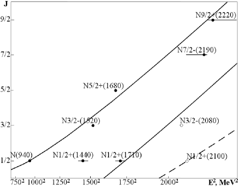
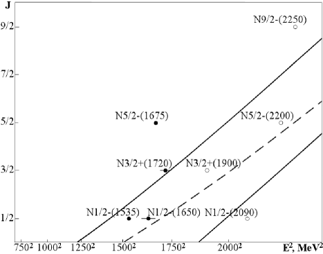
Figure 1: Nucleon resonance Regge trajectories that start with $J^{P}={1/2}^{+}$, calculated using Eqs. (33) and (34) with $m=0.940\,$GeV, $\lambda=0.345\,$GeV². The solid lines are obtained with the quantum number values $n=0$, $N=0$ and $N=2$, the dashed line corresponds to $n=1$, $N=0$. The experimental masses and errors are taken from [17].

Figure 2: Nucleon resonance Regge trajectories that start with $J^{P}={1/2}^{-}$, calculated using the same parameter values as for Fig. 1. The solid lines are obtained from Eq. (33) with $n=0$, $N=1$ and $N=3$, the dashed line results from Eq. (35) with $n=0$, $N=0$.

The calculated Regge trajectories are presented in Figs. 1 and 2. In Fig. 1 we plot the trajectories of $1/2^{+}$, $3/2^{-}$,… states: the nucleon Regge trajectory, its successor with $N=2$ and the first radially excited trajectory with $n=1$, $N=0$. Fig. 2 shows the opposite-parity states: the nucleon successors with $N=1$ and $N=3$ along with the ground-state trajectory ($n=0$, $N=0$) that was calculated using the opposite-parity formula (35). The experimental masses are taken from Particle Data Group [17]. We display the experimental uncertainties if they are high enough. The unclear states for which the approximate masses are only known are depicted by empty circles. From Figs. 1 and 2 one can see that on the plotted trajectories all the $J=1/2$ and $J=3/2$ states below $2100$ MeV correspond to certain experimentally observed resonances. In particular, the $N=2$ and $N=3$ trajectories seem to contain $N_{3/2-}(2080)$ and $N_{1/2-}(2090)$ respectively. In its turn, the radially excited trajectory in Fig. 1 passes through $N_{1/2+}(2100)$.

On the other hand, several states drop out of our systematics. These are the Roper resonance $N_{1/2+}(1440)$, $N_{5/2-}(1675)$ and $N_{9/2-}(2250)$. Actually, the position of the Roper resonance is a longstanding problem since both the conventional three-quark model [18] and quark-diquark scheme [16] treat it as the radial excitation which is unexpected to be lighter than the first negative-parity state $N_{1/2-}(1535)$. To reproduce the correct splitting between $N_{1/2+}(1440)$ and $N_{1/2-}(1535)$, the effects of quark-antiquark pair contributions [19] and of curvature in combination with the approximate conformal symmetry [20] were invoked. Noticeably, all the three states that are dropped out have masses close to those of the states with the same spin and opposite parity, $N_{1/2-}(1535)$, $N_{5/2+}(1680)$ and $N_{9/2-}(2220)$. Thus, in principle, we were able to incorporate the absent states in our description if we assumed that the diquark configuration with opposite parity, i.e. pseudoscalar could occur along with the scalar one at energies above $1400$ MeV. Then the degenerate opposite-parity energy levels would emerge: $N_{1/2+}(1440)$ and $N_{1/2-}(1535)$ etc. However, the accurate treatment of different diquark configurations should incorporate mixing effects [21] that is out of scope of the present work.

A few comments on the parity degeneracy are in order. The systematic parity doubling in excited baryons is usually thought to be a manifestation of effective chiral symmetry restoration in the upper part of the spectrum. However, when treated in different approaches, this phenomenon leads to different multiplet structures of baryon states (see reviews [22, 23]). Under assumption that the $N$ and $\Delta$-resonances fill out the irreducible representations of the parity-chiral group $SU(2)_{L}\otimes SU(2)_{R}\otimes C_{i}$ [24], there appear doublets of the $N$-resonance states (along with multiplets containing also $\Delta$’s). Alternatively, the $O(4)\otimes SU(2)_{I}$ symmetry advocated in Ref.[8] implies that $N$’s fall into the Rarita-Schwinger-like Lorentz multiplets $(K/2,K/2)\otimes[(1/2,0)\oplus(0,1/2)]$ whose dimensionality starts with 3, that is the approximately degenerate triplet $N_{1/2+}(1440)$, $N_{1/2-}(1535)$ and $N_{3/2-}(1520)$. Note that our model relies on the Dirac field transforming according to $(1/2,0)\oplus(0,1/2)$ rather than the Rarita-Schwinger field and thus has nothing to do with the above-discussed multiplets.

Table 1: Comparison between the calculated masses of nucleon resonances and the experimental masses [17]. This work: Eqs. (33)-(35), FK: AdS/QCD model by Forkel and Klempt [25] (values are cited from [26]), CI: Capstick and Isgur [27], BIL: Bijker, Iachello and Leviatan [7], S: quark-diquark model by Santopinto [28], BnA and BnB: Bonn model [29], MK: Skyrme model by Karliner and Mattis [30]. Blanks in ”This work” column are the states that cannot be described in the scalar diquark configuration considered (see Section 5 for discussion).

Resonance	Exp	This work	FK	CI	BIL	S	BnA	BnB	MK
$N(940)$	$940$	$940$	$943$	$960$	939	940	$939$	$939$	$1190$
$N_{1/2+}(1440)$	$1445\pm 25$		$1396$	$1540$	$1444$	$1562$	$1698$	$1540$
$N_{1/2-}(1535)$	$1535\pm 10$	$1424$	$1516$	$1460$	$1563$	$1538$	$1435$	$1470$	$1478$
$N_{1/2-}(1650)$	$1655\pm 15$	$1705$	$1628$	$1535$	1683	1675	$1660$	$1767$
$N_{1/2+}(1710)$	$1710\pm 30$	$1735$	$1735$	$1770$	$1683$	$1640$	$1729$	$1778$	$1427$
$N_{1/2-}(2090)$	$\approx 2090$	$1983$	$2102$	$2135$			$2200$	$2180$
$N_{1/2+}(2100)$	$\approx 2100$	$2098$	$2017$	$1975$			$2127$	$2177$
$N_{3/2-}(1520)$	$1520\pm 5$	$1424$	$1516$	$1495$	$1563$	$1538$	$1476$	$1485$	$1715$
$N_{3/2+}(1720)$	$1725\pm 25$	$1735$	$1735$	$1795$	$1737$	$1675$	$1688$	$1762$	$1982$
$N_{3/2+}(1900)$	$\approx 1900$	$2005$	$1926$	$1870$			$1899$	$1904$
$N_{3/2-}(2080)$	$\approx 2080$	$1983$	$2102$	$2125$			$2079$	$2095$
$N_{5/2-}(1675)$	$1675\pm 5$		$1628$	$1630$	$1683$	$1671$	$1655$	$1622$	$1744$
$N_{5/2+}(1680)$	$1685\pm 5$	$1735$	$1735$	$1770$	$1737$	$1675$	$1723$	$1718$	$1823$
$N_{5/2-}(2200)$	$\approx 2200$	$2252$	$2102$	$2234$			$2185$	$2217$
$N_{7/2-}(2190)$	$2150\pm 50$	$1983$	$2102$	$2090$	$2140$		$2093$	$2100$	$2075$
$N_{9/2+}(2220)$	$2250\pm 50$	$2196$	$2265$	$2327$	$2271$		$2221$	$2221$	$2327$
$N_{9/2-}(2250)$	$\approx 2250$		$2184$	$2234$	$2229$		$2212$	$2170$	$2234$

In Table 1 we list the low-lying states predicted by the present model as well as by some other models. When comparing these results, one should keep in mind that the number of fitting parameters ranges from two in the present, AdS/QCD [25] and Skyrme [30] models to seven in the relativized model [27].

Inspecting Table 1, one observes degenerate states with increasing $J$ among the model predictions. The high degeneracies that occur within the present approach and the AdS/QCD model [25] deserve some explanation. Within the latter model there is $(\ell+n)$-degeneracy where $\ell$ and $n$ are the orbital and radial quantum numbers respectively. This implies that intrinsic orbital and spin angular momenta can be assigned to the observed states – the assumption that is feasible since the spin-orbital coupling is small for baryons. In contrast, our model conserves the total angular momentum $J$ and its part $N$, which is different from the orbital and spin ones and stems from the specific oscillator interaction. The resulting $(J+N)$-degeneracy is a bit weaker than the $(\ell+n)$-degeneracy of the AdS/QCD approach. For example, our model predicts that $N_{5/2-}(2200)$ should be substantially heavier than $N_{1/2-}(2090)$, $N_{3/2-}(2080)$ and $N_{7/2-}(2190)$ which are degenerate in both the models.

6 Conclusion

In this work the exactly solvable three-body oscillator model with the spin-1/2 content has been constructed by employing the extension of the $SL(2,C)$ group to the $Sp(4,C)$ one. The Dirac-like equation for the $Sp(4,C)$ spinors incorporates the ordinary relativistic kinematics, but in the presence of interaction differs significantly from the equations of the other three-body oscillator models, in particular, of the FKR model [1]. The main feature is that the present model includes only one three-dimensional oscillator mode, whereas the remaining degrees of freedom of relative motion are spent to get the rotational excitations. The corresponding quantum number $N$ goes as the addition to the total spin $J$, so that the energy spectrum possesses the $(J+N)$-degeneracy. The application to the nucleon resonance mass spectrum has shown that such a model results in the Regge trajectories $J(E^{2})$ that are asymptotically linear in $E^{2}$ and do not contain any missing states with $J=1/2$ and $J=3/2$ states below $2100$ MeV. Several states such as the Roper resonance drop out of the developed simplistic model, which has only two parameters, the oscillator coupling constant and the nucleon groud-state mass, and uses the scalar diquark configuration solely. Some modifications of the model, in particular, introducing extra interactions may be needed to reproduce the electric form-factors that will be discussed elsewhere.

References

- [1] R. P. Feynman, M. Kislinger, F. Ravndal, Phys. Rev. D 3, 2706 (1971)
- [2] A. N. Mitra, Phys. Rev. D 11, 3270 (1975)
- [3] H. Toki, J. Dey, M. Dey, Phys. Lett. B 133, 20 (1983)
- [4] A. Bohm, M. E. Loewe, P. Magnollay, Phys. Rev. D 32, 791 (1985)
- [5] S. Ishida, K. Yamada, Progr. Theor. Phys. 91, 775 (1994)
- [6] F. Buisseret, C. Semay, Phys. Rev. D 73, 114011 (2006)
- [7] R. Bijker, F. Iachello, A. Leviatan, Annals of Phys. 284, 89 (2000)
- [8] M. Kirchbach, M. Moshinsky, Yu. F. Smirnov, Phys. Rev. D 64, 114005 (2001)
- [9] M. Moshinsky, A. Szczepaniak, J. Phys. A 22, L817 (1989)
- [10] D. A. Kulikov, R. S. Tutik, A. P. Yaroshenko, Phys. Lett. B 644, 311 (2007)
- [11] E. M. Lifshitz, L. P. Pitaevskii, V. I. Berestetskii, Quantum Electrodynamics (Pergamon, Oxford, 1982)
- [12] Ph. Droz-Vincent, Phys. Rev. A 73, 042101 (2006)
- [13] J. P. Elliott, P. G. Dawber, Symmetry in Physics, Vol. 2 (Oxford University Press, New York, 1986)
- [14] A. Selem, F. Wilczek, arXiv: hep-ph/0602128 (2006)
- [15] M. Anselmino, E. Predazzi, S. Ekelin, S. Fredriksson, D.B. Lichtenberg, Rev. Mod. Phys. 65, 1199 (1993)
- [16] A. V. Anisovich, V. V. Anisovich, M. A. Matveev, V. A. Nikonov, A. V. Sarantsev, T. O. Vulfs, Int. J. Mod. Phys. A 25, 2965 (2010)
- [17] J. Beringer et al. (Particle Data Group), Phys. Rev. D 86, 010001 (2012)
- [18] N. Isgur, G. Karl, Phys. Rev. D 19, 2653 (1979)
- [19] M. Nunẽz V., S. Lerma H., P. O. Hess, S. Jesgarz, O. Civitarese and M. Reboiro, Phys. Rev. C 70, 025201 (2004)
- [20] M. Kirchbach, C. B. Compean, Phys. Rev. D 82, 034008 (2010)
- [21] K. Nagata, A. Hosaka, J. Phys. G 32, 777 (2006)
- [22] R. L. Jaffe, D. Pirjol, A. Scardicchio, Phys. Rept. 435, 157 (2006)
- [23] S. S. Afonin, Int. J. Mod. Phys. A 22, 4537 (2007)
- [24] T. D. Cohen, L. Y. Glozman, Phys. Rev. D 65, 016006 (2002)
- [25] H. Forkel, E. Klempt, Phys. Lett. B 679, 77 (2009)
- [26] E. Klempt, Chinese Phys. C 34, 1241 (2010)
- [27] S. Capstick, N. Isgur, Phys. Rev. D 34, 2809 (1986)
- [28] E. Santopinto, Phys. Rev. C 72, 022201 (2005)
- [29] U. Löring, B. Ch. Metsch, H. R. Petry, Eur. Phys. J. A 10, 447 (2001)
- [30] M. Karliner, M. P. Mattis, Phys. Rev. D 34, 1991 (1986)