Blow-up collocation solutions of nonlinear homogeneous Volterra integral equations

Abstract

In this paper, collocation methods are used for detecting blow-up solutions of nonlinear homogeneous Volterra-Hammerstein integral equations. To do this, we introduce the concept of “blow-up collocation solution” and analyze numerically some blow-up time estimates using collocation methods in particular examples where previous results about existence and uniqueness can be applied. Finally, we discuss the relationships between necessary conditions for blow-up of collocation solutions and exact solutions.

1 Introduction

Some engineering and industrial problems are described by explosive phenomena which are modeled by nonlinear integral equations whose solutions exhibit blow-up at finite time (see [1, 2] and references therein). Many authors have studied necessary and sufficient conditions for the existence of such blow-up time. Particularly, in [3, 4, 5, 6, 7], equation

$$y\left(t\right)=\int_{0}^{t}K\left(t,s\right)G\left(y\left(s\right)\right)\,\textrm{d}s,\qquad t\in I:=\left[0,T\right]$$ (1)

was considered. In these works, conditions for the existence of a finite blow-up time, as well as upper and lower estimates of it, were given, although they were not very accurate in some cases.

A way for improving these estimations is to study numerical approximations of the solution; in this aspect, collocation methods have proven to be a very suitable technique for approximating nonlinear integral equations, because of its stability and accuracy (see [8]). Hence, the aim of this paper is to test the usefulness of collocation methods for detecting blow-up solutions of the nonlinear homogeneous Volterra-Hammerstein integral equation (HVHIE) given by equation (1).

Very recently, Yang and Brunner [9] analysed the blow-up behavior of collocation solutions for a similar Hammerstein-Volterra integral equation with a convolution kernel

$$y(t)=\phi(t)+\int_{0}^{t}K(t-s)G(s,y(s))\textrm{d}s,\qquad t\in I.$$ (2)

Equation (1) should not be regarded as a particular case of (2) (for a convolution kernel), because in [9] a positive non-homogeneity $\phi(t)$ and a Lipschitz-continuous nonlinearity $G$ were considered. Indeed, under the hypotheses on the kernel and the nonlinearity considered in [9], it is well-known that equation (1) has only the trivial solution ($y\equiv 0$) and moreover, under the conditions we shall state in Section 3, the collocation equations given in [9] lead to the trivial sequence ($y_{n}=0$ for all $n\in\mathbb{N}$). Thus, equation (1) considered here is beyond the scope of the standard techniques, which usually impose conditions that guarantee the uniqueness of the solutions.

An approach for solving this problem, which we shall follow in this paper, is writing equation (1) as an implicitly linear homogeneous Volterra integral equation (HVIE), i.e. setting $z=G\circ y$ and plugging it into the nonlinear integral equation (1) to obtain

$$z(t)=G\left(\left(\mathcal{V}z\right)\left(t\right)\right)=G\left(\int_{0}^{t}K\left(t,s\right)z(s)\,\textrm{d}s\right),\qquad t\in I,$$ (3)

being $\mathcal{V}$ the linear Volterra operator. There is a one-to-one correspondence between solutions of (1) and (3) (see [8, 10]), in particular, if $z$ is a solution of (3), then $y:=\mathcal{V}z$ is a solution of (1).

This paper is structured as follows: in Section 2 we introduce briefly the basic definitions and state the notation. Next, we devote Section 3 to generalize the results about existence and uniqueness of nontrivial collocation solutions obtained in [11] in order to apply the results to blow-up problems. In Section 4, we introduce the concept of “blow-up collocation solution” and analyse numerically some blow-up time estimates using collocation methods in particular examples where the previous results about existence and uniqueness can be applied. Finally, in Section 5, we discuss the relationships between necessary conditions for blow-up of collocation solutions and exact solutions.

2 Collocation problems for implicitly linear HVIEs

Following the notation of [8], a collocation problem for equation (3) is given by a mesh $I_{h}:=\left\{t_{n}\,:\,\,0=t_{0}<t_{1}<\ldots<t_{N}=T\right\}$ and a set of $m$ collocation parameters $0\leq c_{1}<\ldots<c_{m}\leq 1$. We denote $h_{n}:=t_{n+1}-t_{n}$ $(n=0,\ldots,N-1)$ and the quantity $h:=\textrm{max}\left\{h_{n}\,:\,\,0\leq n\leq N-1\right\}$ is the diameter of $I_{h}$. Moreover, the collocation points are given by $t_{n,i}:=t_{n}+c_{i}h_{n}$ $(i=1,\ldots,m)$, and the set of collocation points is denoted by $X_{h}$ (see [8, 12]). A collocation solution $z_{h}$ is then given by the collocation equation

$$z_{h}\left(t\right)=G\left(\int_{0}^{t}K\left(t,s\right)z_{h}\left(s\right)\,\textrm{d}s\right),\qquad t\in X_{h}\,,$$

where $z_{h}$ is in the space of piecewise polynomials of degree less than $m$.

From now on, a “collocation problem” or a “collocation solution” will be always referred to the implicitly linear HVIE (3). So, if we want to obtain an estimation of a solution of the nonlinear HVHIE (1), then we have to consider $y_{h}:=\mathcal{V}z_{h}$.

At the beginning of Section 4, we define the concepts of “blow-up collocation problems” and “blow-up collocation solutions”. To do this, we extend the definition of “collocation solution” to meshes $I_{h}$ with infinite points. Taking this into account, it is noteworthy that if $z_{h}$ is a blow-up collocation solution, then $y_{h}$ also blows up at the same blow-up time.

As it is stated in [8], a collocation solution $z_{h}$ is completely determined by the coefficients $Z_{n,i}:=z_{h}\left(t_{n,i}\right)$ $(n=0,\ldots,N-1)$ $(i=1,\ldots,m)$, since $z_{h}\left(t_{n}+vh_{n}\right)=\sum_{j=1}^{m}L_{j}\left(v\right)Z_{n,j}$ for all $v\in\left]0,1\right]$, where $L_{1}\left(v\right):=1$, $L_{j}\left(v\right):=\prod_{k\neq j}^{m}\frac{v-c_{k}}{c_{j}-c_{k}}$ $(j=2,\ldots,m)$ are the Lagrange fundamental polynomials with respect to the collocation parameters. The values of $Z_{n,i}$ are given by the system

$$Z_{n,i}=G\left(F_{n}\left(t_{n,i}\right)+h_{n}\sum_{j=1}^{m}B_{n}\left(i,j\right)Z_{n,j}\right),$$ (4)

where

$$B_{n}\left(i,j\right):=\int_{0}^{c_{i}}K\left(t_{n,i},t_{n}+sh_{n}\right)L_{j}\left(s\right)\,\textrm{d}s$$

and

$$F_{n}\left(t\right):=\int_{0}^{t_{n}}K\left(t,s\right)z_{h}\left(s\right)\,\textrm{d}s.$$ (5)

The term $F_{n}\left(t_{n,i}\right)$ is called the lag term.

3 Existence and uniqueness of nontrivial collocation solutions

In [11], we used collocation methods for approximating the nontrivial solutions of (1). In particular, we studied the collocation solutions of the implicitly linear HVIE (3), and assuming that some general conditions were held. Specifically, it was required that the kernel $K$ was a locally bounded function; nevertheless, non locally bounded kernels, e.g. weakly singular kernels, appear in many cases of blow-up solutions (see [7]) and so, in the present work, we shall first replace this condition with another not excluding this kind of kernels. Hence, the general conditions that we are going to impose (even if they are not explicitly mentioned) are:

• Over $K$. The kernel $K:\mathbb{R}^{2}\to\left[0,+\infty\right[$ has its support in $\left\{\left(t,s\right)\in\mathbb{R}^{2}\,:\,0\leq s\leq t\right\}$.

  For every $t>0$, the map $s\mapsto K\left(t,s\right)$ is locally integrable, and $\mathcal{K}(t):=\int_{0}^{t}K\left(t,s\right)\textrm{d}s$ is a strictly increasing function. Moreover, $\lim_{t\rightarrow a^{+}}\int_{a}^{t}K\left(t,s\right)\,\textrm{d}s=0$ for all $a\geq 0$. Note that for convolution kernels (i.e. $K(t,s)=k(t-s)$) this last condition is always held, because $k$ is locally integrable and then

  $$\lim_{t\rightarrow a^{+}}\int_{a}^{t}k(t-s)\,\textrm{d}s=\lim_{t\rightarrow a^{+}}\int_{0}^{t-a}k(s)\,\textrm{d}s=\lim_{t\rightarrow 0^{+}}\int_{0}^{t}k(s)\,\textrm{d}s=0.$$

• Over $G$. The nonlinearity $G:\left[0,+\infty\right[\to\left[0,+\infty\right[$ is a continuous, strictly increasing function, and $G(0)=0$.

Note that, since $G$ is injective, the solution $y$ of equation (1) is also given by $y=G^{-1}\circ z$, where $z$ is a solution of (3). Also, since $G(0)=0$, the zero function is always a solution of both equations (1) and (3), called trivial solution. Moreover, for convolution kernels, given a solution $z(t)$ of (3), any horizontal translation of $z$, $z_{c}(t)$ defined by

$$z_{c}(t)=\begin{cases}0,&\text{if }t<c\\ z(t-c)&\text{if }t\geq c,\\ \end{cases}$$

is also a solution of (3) (see [14, 13, 11]). Motivated by this fact we give the next definitions, that are also valid for nonconvolution kernels:

Definition 3.1

We say that a property $\mathcal{P}$ holds near zero if there exists $\epsilon>0$ such that $\mathcal{P}$ holds on $\left]0,\delta\right[$ for all $0<\delta<\epsilon$. On the other hand, we say that $\mathcal{P}$ holds away from zero if there exists $\tau>0$ such that $\mathcal{P}$ holds on $\left]t,+\infty\right[$ for all $t>\tau$.

The concept “away from zero” was originally defined in a more restrictive way in [11]; nevertheless both definitions are appropriate for our purposes.

Definition 3.2

We say that a solution of (3) is nontrivial if it is not identically zero near zero. Moreover, given a collocation problem, we say that a collocation solution is nontrivial if it is not identically zero in $\left]t_{0},t_{1}\right]$.

Given a kernel $K$, a nonlinearity $G$ and some collocation parameters $\left\{c_{1},\ldots,c_{m}\right\}$, in [11] there were defined three kinds of existence of nontrivial collocation solutions (of the corresponding collocation problem) in an interval $I=\left[0,T\right]$ using a mesh $I_{h}$: existence near zero, existence for fine meshes, and unconditional existence. For these two last kinds of existence, it is ensured the existence of nontrivial collocation solutions in any interval, and hence, there is no blow-up. On the other hand, “existence near zero” is equivalent to the existence of a nontrivial collocation solution with adaptive stepsize, as it is defined in [9]. In this case, collocation solutions can always be extended a little more, but it is not ensured the existence of nontrivial collocation solutions for arbitrarily large $T$ and, thus, it can blow up in finite time.

As in [11], we shall restrict our analysis to two particular cases of collocation problems, namely:

• Case 1: $m=1$ with $c_{1}>0$.

• Case 2: $m=2$ with $c_{1}=0$.

In these cases, system (4) is reduced to a single nonlinear equation, whose solution is given by the fixed points of $G\left(\alpha+\beta y\right)$ for some $\alpha,\beta$. Determining conditions for the existence of collocation solutions in the general case is a problem of an overwhelming difficulty. In fact, in [11] examples of equations for which, in cases 1 and 2, there existed nontrivial collocation solutions, yet in other some other cases, for the same equation, there were no nontrivial collocation solutions, were given.

The proofs of the results obtained in [11] rely on the locally boundedness of the kernel $K$. Therefore, we will revise such proofs, imposing the new general conditions given at the beginning of this section, and avoiding other hypotheses that turn out to be unnecessary. For example, we extend these results to decreasing convolution kernels, among others.

As in the previous work [11], we will need a Lemma on nonlinearities $G$ satisfying the general conditions:

Lemma 3.1

The following statements are equivalent to the statement that $\frac{G\left(y\right)}{y}$ is unbounded (in $\left]0,+\infty\right[$):

• There exists $\beta_{0}>0$ such that $G\left(\beta y\right)$ has nonzero fixed points for all $0<\beta\leq\beta_{0}$.

• Given $A\geq 0$, there exists $\beta_{A}>0$ such that $G\left(\alpha+\beta y\right)$ has nonzero fixed points for all $0\leq\alpha\leq A$ and for all $0<\beta\leq\beta_{A}$.

3.1 Case 1: $m=1$ with $c_{1}>0$

First, we shall consider $m=1$ with $c_{1}>0$. Equations (4) are then reduced to

$$Z_{n,1}=G\left(F_{n}\left(t_{n,1}\right)+h_{n}B_{n}Z_{n,1}\right)\qquad(n=0,\ldots,N-1),$$ (6)

where

$$B_{n}:=B_{n}\left(1,1\right)=\int_{0}^{c_{1}}K\left(t_{n,1},t_{n}+sh_{n}\right)\,\textrm{d}s$$ (7)

and the lag terms $F_{n}\left(t_{n,1}\right)$ are given by (5) with $i=1$. Note that $B_{n}>0$ because the integrand in (7) is strictly positive almost everywhere in $\left]0,c_{1}\right[$.

Remark 3.1

In [11], it is ensured that $\lim_{h_{n}\rightarrow 0^{+}}h_{n}B_{n}=0$ taking into account (7) and the old general conditions imposed over $K$. Thus, we must ensure that the limit also vanishes considering the new general conditions. In fact, with a change of variable, we can express (7) as

$$B_{n}=\frac{1}{h_{n}}\int_{t_{n}}^{t_{n,1}}K\left(t_{n,1},s\right)\,\textrm{d}s.$$ (8)

Hence, by (8) and the new condition, we have

$$\lim_{h_{n}\rightarrow 0^{+}}h_{n}B_{n}=\lim_{t\rightarrow t_{n}^{+}}\int_{t_{n}}^{t}K\left(t,s\right)\,\textrm{d}s=0,$$

since $t_{n,1}=t_{n}+c_{1}h_{n}$.

Now, we are in position to give a characterization of the existence near zero of nontrivial collocation solutions:

Proposition 3.1

There is existence near zero if and only if $\frac{G\left(y\right)}{y}$ is unbounded.

Proof.

($\Leftarrow$) Let us prove that if $\frac{G\left(y\right)}{y}$ is unbounded, then there is existence near zero. So, we are going to prove by induction over $n$ that there exist $H_{n}>0$ $\left(n=0,\ldots,N-1\right)$ such that if $0<h_{n}\leq H_{n}$ then there exist solutions of the system (6) with $Z_{0,1}>0$:

• For $n=0$, taking into account Remark 3.1 and Lemma 3.1-(i) (see below), we choose a small enough $H_{0}>0$ such that $0<h_{0}B_{0}\leq\beta_{0}$ for all $0<h_{0}\leq H_{0}$. So, since the lag term is $0$, we can apply Lemma 3.1-(i) to the equation (6), concluding that there exist strictly positive solutions for $Z_{0,1}$.

• Let us suppose that, choosing one of those $Z_{0,1}$ and given $n>0$, there exist $H_{1},\ldots,$ $H_{n-1}>0$ such that if $0<h_{i}\leq H_{i}$ ($i=1,\ldots,n-1$) then there exist coefficients $Z_{1,1},\ldots,Z_{n-1,1}$ fulfilling the equation (6). Note that these coefficients are strictly positive, and hence, it is guaranteed that the corresponding collocation solution $z_{h}$ is (strictly) positive in $\left]0,t_{n}\right]$.

• Finally, we are going to prove that there exists $H_{n}>0$ such that if $0<h_{n}\leq H_{n}$ then there exists $Z_{n,1}>0$ fulfilling the equation (6) with the previous coefficients $Z_{0,1},\ldots Z_{n-1,1}$:

  Let us define

  $$A:=\max\left\{F_{n}\left(t_{n}+c_{1}\epsilon\right)\,:\,0\leq\epsilon\leq 1\right\}.$$

  Note that $A$ exists because $s\mapsto K\left(t,s\right)$ is locally integrable for all $t>0$, and $z_{h}$ is bounded in $\left[0,t_{n}\right]$; hence, $F_{n}$ (see (5)) is bounded in $\left[t_{n},t_{n}+c_{1}\right]$. Moreover, $A\geq 0$ because $K$ and $z_{h}$ are positive functions.

  So, applying Lemma 3.1-(ii) (see below), there exists $\beta_{A}>0$ such that $G\left(\alpha+\beta y\right)$ has nonzero (strictly positive) fixed points for all $0\leq\alpha\leq A$ and for all $0<\beta\leq\beta_{A}$. On one hand, taking into account Remark 3.1, we choose a small enough $0<H_{n}\leq 1$ such that $0<h_{n}B_{n}\leq\beta_{A}$ for all $0<h_{n}\leq H_{n}$; on the other hand, choosing one of those $h_{n}$, we have $0\leq F\left(t_{n,1}\right)\leq A$. Hence, we obtain the existence of $Z_{n,1}$ as the strictly positive fixed point of $G\left(F\left(t_{n,1}\right)+h_{n}B_{n}y\right)$.

($\Rightarrow$) For proving the other condition, we use Lemma 3.1-(i), taking into account Remark 3.1. ∎

A similar result was proved in [11] with the additional hypothesis “$K\left(t,s\right)\leq K\left(t^{\prime},s\right)$ for all $0\leq s\leq t<t^{\prime}$” (or “$k$ is increasing” for the particular case of convolution kernels $K(t,s)=k(t-s)$). We have shown that this hypothesis is not needed and the difference between the proofs is the choice of $A$.

Taking into account Remark 3.1, we can adapt the results given in [11] about sufficient conditions on existence for fine meshes and unconditional existence to our new general conditions. This will help us to identify collocation problems without blow-up (see Proposition 3.2 below).

In the following results recall the Definition 3.1 of the concepts “near zero” and “away from zero”.

Proposition 3.2

Let $\frac{G(y)}{y}$ be unbounded near zero.

• If $K$ is a convolution kernel and $\frac{G(y)}{y}$ is bounded away from zero, then there is existence for fine meshes.

• If $\frac{y}{G(y)}$ is unbounded away from zero, then there is unconditional existence.

If, in addition, $\frac{G(y)}{y}$ is a strictly decreasing function, then there is at most one nontrivial collocation solution.

The proof is analogous to the one given in [11]. Note that the property “$\frac{y}{G(y)}$ is unbounded away from zero” appears there as “there exists a sequence $\left\{y_{n}\right\}_{n=1}^{+\infty}$ of positive real numbers and divergent to $+\infty$ such that $\lim_{n\rightarrow+\infty}\frac{G\left(y_{n}\right)}{y_{n}}=0$”, but both are equivalent.

3.2 Case 2: $m=2$ with $c_{1}=0$

Considering $m=2$ with $c_{1}=0$, we have to solve the following equations:

$$Z_{n,1} = G\left(F_{n}\left(t_{n,1}\right)\right)$$ (9)

$$Z_{n,2} = G\left(F_{n}\left(t_{n,2}\right)+h_{n}B_{n}\left(2,1\right)Z_{n,1}+h_{n}B_{n}\left(2,2\right)Z_{n,2}\right),$$ (10)

for $n=0,\ldots,N-1$, where

$$B_{n}\left(2,j\right)=\int_{0}^{c_{2}}K\left(t_{n,2},t_{n}+sh_{n}\right)L_{j}\left(s\right)\,\textrm{d}s,\qquad(j=1,2)$$ (11)

and $F_{n}\left(t_{n,i}\right)$ $(i=1,2)$ are given by (5). Note that $B_{n}\left(2,j\right)>0$ for $j=1,2$, because the integrand in (11) is strictly positive almost everywhere in $\left]0,c_{2}\right[$.

Remark 3.2

As in the first case, we have to ensure that $\lim_{h_{n}\rightarrow 0^{+}}h_{n}B_{n}\left(2,j\right)=0$ for $j=1,2$, taking into account the new general conditions (see Remark 3.1). Actually, since $0<L_{j}\left(s\right)<1$ for $s\in\left]0,c_{2}\right[$, we have

$$0\leq h_{n}B_{n}\left(2,j\right)\leq h_{n}\int_{0}^{c_{2}}K\left(t_{n,2},t_{n}+sh_{n}\right)\,\textrm{d}s=\int_{t_{n}}^{t_{n,2}}K\left(t_{n,2},s\right)\,\textrm{d}s.$$ (12)

Hence, by (12) and the new condition, the following inequalities are fulfilled:

$$0\leq\lim_{h_{n}\rightarrow 0^{+}}h_{n}B_{n}\left(2,j\right)\leq\lim_{t\rightarrow t_{n}^{+}}\int_{t_{n}}^{t}K\left(t,s\right)\,\textrm{d}s=0.$$

Analogously to the previous case, we present a characterization of the existence near zero of nontrivial collocation solutions:

Proposition 3.3

Let the map $t\mapsto K\left(t,s\right)$ be continuous in $\left]s,\epsilon\right[$ for some $\epsilon>0$ and for all $0\leq s<\epsilon$ (this hypothesis can be removed if $c_{2}=1$). Then there is existence near zero if and only if $\frac{G\left(y\right)}{y}$ is unbounded.

Proof.

($\Leftarrow$) Let us prove that if $\frac{G\left(y\right)}{y}$ is unbounded, then there is existence near zero. So, we are going to prove by induction over $n$ that there exist $H_{n}>0$ $\left(n=0,\ldots,N-1\right)$ such that if $0<h_{n}\leq H_{n}$ then there exist solutions of the system (10) with $Z_{0,2}>0$:

• For $n=0$, taking into account Remark 3.2 and Lemma 3.1-(i), we choose a small enough $H_{0}>0$ such that $0<h_{0}B_{0}\left(2,2\right)\leq\beta_{0}$ for all $0<h_{0}\leq H_{0}$. So, since the lag terms are $0$ and $Z_{0,1}=G\left(0\right)=0$, we can apply Lemma 3.1-(i) to the equation (10), concluding that there exist strictly positive solutions for $Z_{0,2}$.

• Let us suppose that, choosing one of those $Z_{0,2}$ and given $n>0$, there exist constants $H_{1},\ldots,H_{n-1}>0$ such that if $0<h_{i}\leq H_{i}$ ($i=1,\ldots,n-1$) then there exist coefficients $Z_{1,2},\ldots,Z_{n-1,2}$ fulfilling the equation (10). Moreover, let us suppose that $z_{h}$ is positive in $\left[0,t_{n}\right]$, i.e. these coefficients satisfy $Z_{l,2}\geq\left(1-c_{2}\right)Z_{l,1}\geq 0$ for $l=1,\ldots,n-1$, where $Z_{l,1}$ is given by (9).

• Finally, we are going to prove that there exists $H_{n}>0$ such that if $0<h_{n}\leq H_{n}$ then there exists $Z_{n,2}>0$ fulfilling the equation (10) with the previous coefficients, and $z_{h}$ is positive in $\left[0,t_{n+1}\right]$, i.e. $Z_{n,2}\geq\left(1-c_{2}\right)Z_{n,1}\geq 0$:

  Let us define

  $$A := \max\left\{F_{n}\left(t_{n}+c_{2}\epsilon\right)+\right.$$

  $$\left.\epsilon G\left(F_{n}\left(t_{n}+c_{1}\epsilon\right)\right)\int_{0}^{c_{2}}K\left(t_{n,2},t_{n}+sh_{n}\right)L_{1}\left(s\right)\,\textrm{d}s\,:\,0\leq\epsilon\leq 1\right\}.$$

  Note that $A$ exists and $A\geq 0$ because $s\mapsto K\left(t,s\right)$ is locally integrable for all $t>0$, $z_{h}$ is bounded and positive in $\left[0,t_{n}\right]$, the nonlinearity $G$ is bounded and positive, and the polynomial $L_{1}$ is bounded and positive in $\left[0,c_{2}\right]$.

  So, applying Lemma 3.1-(ii), there exists $\beta_{A}>0$ such that $G\left(\alpha+\beta y\right)$ has nonzero (strictly positive) fixed points for all $0\leq\alpha\leq A$ and for all $0<\beta\leq\beta_{A}$. On one hand, taking into account Remark 3.2, we choose a small enough $0<H_{n}\leq 1$ such that $0<h_{n}B_{n}(2,2)\leq\beta_{A}$ for all $0<h_{n}\leq H_{n}$; on the other hand, taking into account (5), the lag terms $F_{n}\left(t_{n,i}\right)$ are positive for $i=1,2$, because $K$ and $z_{h}$ are positive. Therefore, by (9), $Z_{n,1}=G\left(F_{n}\left(t_{n,1}\right)\right)$ is positive, because $G$ is positive. Moreover, $h_{n}B_{n}\left(2,1\right)$ is positive. So,

  $$0\leq F_{n}\left(t_{n,2}\right)+h_{n}B_{n}\left(2,1\right)Z_{n,1}\leq A.$$

  Hence, we obtain the existence of $Z_{n,2}$ as the strictly positive fixed point of the function $G\left(\alpha+\beta y\right)$ where $\alpha:=F_{n}\left(t_{n,2}\right)+h_{n}B_{n}\left(2,1\right)Z_{n,1}$ and $\beta:=h_{n}B_{n}(2,2)$.

  Concluding, we have to check that $Z_{n,2}\geq\left(1-c_{2}\right)Z_{n,1}$. On one hand,

  $$Z_{n,2}=G\left(F_{n}\left(t_{n,2}\right)+h_{n}\sum_{j=1}^{2}B_{n}\left(2,j\right)Z_{n,j}\right)\geq G\left(F_{n}\left(t_{n,2}\right)\right)$$

  because $B_{n}\left(2,j\right)Z_{n,j}\geq 0$ for $j=1,2$. On the other hand, since $t\mapsto K\left(t,s\right)$ is continuous in $\left]s,\epsilon\right[$ for some $\epsilon>0$ and for all $0\leq s<\epsilon$, we can suppose that the stepsize is small enough for $t_{n,1}<\epsilon$, and then $F_{n}(t)$ is continuous in $t_{n,1}$ (see 5). Hence, since $G$ is continuous, $G\left(F_{n}(t)\right)$ is also continuous in $t_{n,1}$, i.e. $\lim_{h_{n}\rightarrow 0^{+}}G\left(F_{n}\left(t_{n,2}\right)\right)=G\left(F_{n}\left(t_{n,1}\right)\right)$. Therefore, choosing a small enough $h_{n}$, we have

  $$G\left(F_{n}\left(t_{n,2}\right)\right)\geq\left(1-c_{2}\right)G\left(F_{n}\left(t_{n,1}\right)\right)=\left(1-c_{2}\right)Z_{n,1}.$$

($\Rightarrow$) For proving the other condition, we use Lemma 3.1-(i), taking into account Remark 3.2. ∎

It is noteworthy that a similar result was proved in [11], but the hypothesis on the kernel was “$K\left(t,s\right)\leq K\left(t^{\prime},s\right)$ for all $0\leq s\leq t<t^{\prime}$”, and so, unlike Proposition 3.3, it could not be applied to decreasing convolution kernels (for example). Again, the main difference between both proofs lies in the choice of $A$.

Note that for convolution kernels $K(t,s)=k(t-s)$, the hypothesis on $K$ is equivalent to say that $k$ is continuous near zero, which is a fairly weak hypothesis. On the other hand, for general kernels, this hypothesis is only needed to ensure that $t\mapsto K\left(t,s\right)$ is continuous in $t_{n,1}$. Therefore, if it is not continuous, it is important to choose $h_{i}$ such that the mapping $t\mapsto K\left(t,s\right)$ is continuous at the collocation points $t_{i,1}$ $(i=0,\ldots N-1)$. More specifically, the hypothesis on $K$ is only needed to check that $Z_{n,2}\geq\left(1-c_{2}\right)Z_{n,1}$, and hence, to ensure that $z_{h}$ is positive in $\left[0,t_{n}\right]$. Nevertheless, this hypothesis is not needed to verify that $Z_{0,2}>Z_{0,1}=0$, and so, it is always ensured the existence of $Z_{1,2}$ (and obviously $Z_{1,1}$), even if the hypothesis does not hold. Hence, if we use another method to check that $Z_{1,2}\geq\left(1-c_{2}\right)Z_{1,1}$ (e.g., numerically), then it is ensured the existence of $Z_{2,2}$. Repeating this reasoning we can guarantee the existence of $Z_{n,2}$, removing the hypothesis on $K$. Thus, we can state a result analogous to Proposition 3.3 without hypothesis on the kernel:

Proposition 3.4

$\frac{G\left(y\right)}{y}$ is unbounded if and only if there exists $H_{0}>0$ such that there are nontrivial collocation solutions in $\left[0,t_{1}\right]$ for $0<h_{0}\leq H_{0}$. In this case, there always exists $H_{1}>0$ such that there are nontrivial collocation solutions in $\left[0,t_{2}\right]$ for $0<h_{1}\leq H_{1}$.

Moreover, if $\frac{G\left(y\right)}{y}$ is unbounded and there is a positive nontrivial collocation solution in $\left[0,t_{n}\right]$, then there exists $H_{n}>0$ such that there are nontrivial collocation solutions in $\left[0,t_{n+1}\right]$ for $0<h_{n}\leq H_{n}$.

Considering Remark 3.2 and taking the coefficient $A$ given in (• ‣ 3.2), we can adapt some results of [11] about sufficient conditions on existence for fine meshes and unconditional existence to our new general conditions. These results are useful for identifying collocation problems without blow-up.

Proposition 3.5

Let $\frac{G(y)}{y}$ be unbounded near zero, and let the map $t\mapsto K\left(t,s\right)$ be continuous in $\left]s,\epsilon\right[$ for some $\epsilon>0$ and for all $0\leq s<\epsilon$ (this hypothesis can be removed if $c_{2}=1$).

• If $K$ is a convolution kernel and $\frac{G(y)}{y}$ is bounded away from zero, then there is existence for fine meshes.

• If $\frac{y}{G(y)}$ is unbounded away from zero, then there is unconditional existence.

If, in addition, $\frac{G(y)}{y}$ is a strictly decreasing function, then there is at most one nontrivial collocation solution.

Moreover, as in Proposition 3.4, we can state a result about unconditional existence without hypothesis on the kernel:

Proposition 3.6

Let $\frac{G\left(y\right)}{y}$ be unbounded near zero.

If $\frac{y}{G(y)}$ is unbounded away from zero and there is a positive nontrivial collocation solution in $\left[0,t_{n}\right]$, then there is a nontrivial collocation solution in $\left[0,t_{n+1}\right]$ for any $h_{n}>0$.

If, in addition, $\frac{G\left(y\right)}{y}$ is a strictly decreasing function, then there is at most one nontrivial collocation solution.

3.3 Nondivergent existence and uniqueness

Our interest is the study of existence of nontrivial collocation solutions using meshes $I_{h}$ with arbitrarily small $h>0$. So, we are not interested in collocation problems whose collocation solutions “escape” to $+\infty$ when a certain $h_{n}\rightarrow 0^{+}$, since this is a divergence symptom. Following this criterion, we define the concept of “nondivergent existence”:

Let $0=t_{0}<\ldots<t_{n}$ be a mesh such that there exist nontrivial collocation solutions, and let $S_{h_{n}}$ be the index set of the nontrivial collocation solutions of the corresponding collocation problem with mesh $t_{0}<\ldots<t_{n}<t_{n}+h_{n}$. Given $s\in S_{h_{n}}$, we denote by $Z_{s;n,i}$ the coefficients of the corresponding nontrivial collocation solution verifying equations (4). Then, we say that there is nondivergent existence in $t_{n}^{+}$ if

$$\inf_{s\in S_{h_{n}}}\left\{\max_{i=1,\ldots,m}\left\{Z_{s;n,i}\right\}\right\}$$

exists for small enough $h_{n}>0$ and it does not diverge to $+\infty$ when $h_{n}\rightarrow 0^{+}$. Given a mesh $I_{h}=\left\{0=t_{0}<\ldots<t_{N}\right\}$ such that there exist nontrivial collocation solutions, we say that there is nondivergent existence if there is nondivergent existence in $t_{n}^{+}$ for $n=0,\ldots,N$. See [11] for a more detailed analysis, where we also define the concept of nondivergent uniqueness.

In [11] it is proved the next result:

Proposition 3.7

In cases 1 and 2 with existence of nontrivial collocation solutions, there is nondivergent existence if and only if $\frac{G\left(y\right)}{y}$ is unbounded near zero.

If, in addition, $G$ is “well-behaved”, then there is nondivergent uniqueness.

We say that $G$ is “well-behaved” if $\frac{G\left(\alpha+y\right)}{y}$ is strictly decreasing near zero for all $\alpha>0$. Note that this condition is very weak (see [11]).

So, taking into account Propositions 3.1, 3.3 and 3.7, the main result of this paper is:

Theorem 3.1

(Hypothesis only for case 2 with $c_{2}\neq 1$: the map $t\mapsto K\left(t,s\right)$ is continuous in $\left]s,\epsilon\right[$ for some $\epsilon>0$ and for all $0\leq s<\epsilon$.)

There is nondivergent existence near zero if and only if $\frac{G\left(y\right)}{y}$ is unbounded near zero.

If, in addition, $G$ is “well-behaved” then, there is nondivergent uniqueness near zero.

In the same way, we can combine Propositions 3.4 and 3.7 obtaining a result about nondivergent existence and uniqueness without hypothesis on the kernel, and, as Theorem 3.1, it can be useful to study numerically problems with decreasing convolution kernels in case 2 with $c_{2}\neq 1$.

We can also combine Propositions 3.2, 3.5 and 3.6 with Proposition 3.7, obtaining results about nondivergent existence and uniqueness (for fine meshes and unconditional) that are useful for identifying collocation problems without blow-up. Some of these results can be reformulated as necessary conditions for the existence of blow-up (see Section 5).

4 Blow-up collocation solutions

In this section we will extend the concept of collocation problem and collocation solution in order to consider the case of “blow-up collocation solutions”.

Definition 4.1

We say that a collocation problem is a blow-up collocation problem (or has a blow-up) if the following conditions are held:

1. There exists $T>0$ such that there is no collocation solution in $I=\left[0,T\right]$ for any mesh $I_{h}$.

2. Given $M>0$ there exists $0<\tau<T$, and a collocation solution $z_{h}$ defined on $\left[0,\tau\right]$ such that $|z_{h}(t)|>M$ for some $t\in[0,\tau]$.

We can not speak about “blow-up collocation solutions” in the classic sense, since “collocation solutions” are defined in compact intervals and obviously they are bounded; so, we have to extend first the concept of “collocation solution” to open intervals $I=\left[0,T\right[$ before we are in position to define the notion of “blow-up collocation solution”.

Definition 4.2

Let $I:=[0,T[$ and $I_{h}$ be an infinite mesh given by a strictly increasing sequence $\left\{t_{n}\right\}_{n=0}^{+\infty}$ with $t_{0}=0$ and convergent to $T$.

• A collocation solution on $I$ using the mesh $I_{h}$ is a function defined on $I$ such that it is a collocation solution (in the classic sense) for any finite submesh $\left\{t_{n}\right\}_{n=0}^{N}$ with $N\in\mathbb{N}$.

• A collocation solution on $I$ is a blow-up collocation solution (or has a blow-up) with blow-up time $T$ if it is unbounded.

Remark 4.1

In [9] it is defined the concept of collocation solution with adaptive stepsize that uses an infinite mesh $I_{h}$. It is stated that this kind of collocation solutions blows up in finite time if

$$T_{b}(I_{h}):=\lim_{n\rightarrow\infty}t_{n}=\lim_{n\rightarrow\infty}\sum_{i=0}^{n}h_{i}<\infty,$$

without imposing any condition about unboundedness on the collocation solution. In this case, $T_{b}(I_{h})$ is called the numerical blow-up time. According to this definition, we could remove the second point in Definition 4.1. However, this definition of numerical blow-up time in [9] is made in the framework of a Lipschitz nonlinearity $G$ in the non-homogenous case, and it is proved (in case 1) that the corresponding collocation solution is effectively unbounded if we choose a given adaptive stepsize that depends on the Lipschitz constant of $G$. Nevertheless, we can not use this framework in our case (homogeneous case), because supposing a Lipschitz-continuous nonlinearity $G$ would imply that the unique solution of (1) or (3) is the trivial one. On the other hand, if we consider a non-Lipschitz nonlinearity, then we can not assure that the collocation solution is unbounded since the adaptive stepsize given in [9] becomes zero in the homogeneous case. Therefore, in Definition 4.1 it is necessary the condition about unboundedness, and in Definition 4.2 we impose explicitly that the collocation solution has to be unbounded.

Given a collocation problem with nondivergent uniqueness near zero, a necessary condition for the nondivergent collocation solution to blow-up is that there is neither existence for fine meshes nor unconditional existence. So, for example, given a convolution kernel $K(t,s)=k(t-s)$, in cases 1 and 2 we must require that $\frac{G\left(y\right)}{y}$ is unbounded away from zero (moreover, in case 2 with $c_{2}\neq 1$, we must demand that there exists $\epsilon>0$ such that $k$ is continuous in $\left]0,\epsilon\right[$).

For instance, in [5] it is studied equation (1) with convolution kernel $k(t-s)=(t-s)^{\beta}$, $\beta\geq 0$, and nonlinearity $G(y)=t^{\alpha}$, $0<\alpha<1$, concluding that the nontrivial (exact) solution does not have blow-up. If we consider a collocation problem with the above kernel and nonlinearity in cases 1 and 2, then we can ensure unconditional nondivergent uniqueness (by Propositions 3.2, 3.5 and 3.7); thus, we can also conclude that the nondivergent collocation solution has no blow-up. Actually, we reach the same conclusion considering any kernel satisfying the general conditions (in case 1 and case 2 with $c_{2}=1$) and such that $t\mapsto K\left(t,s\right)$ is continuous in $\left]s,\epsilon\right[$ for some $\epsilon>0$ and for all $0\leq s<\epsilon$ (in case 2 with $c_{2}\neq 1$). In Section 5 we discuss in more detail the relationships between necessary conditions for blow-up of collocation solutions and exact solutions.

4.1 Numerical algorithms

First we need to recall the definition of existence near zero, mentioned at the beginning of Section 3, and given in [11]. It is equivalent to the existence of a nontrivial collocation solution with adaptive stepsize, whose definition is given in [9].

Definition 4.3

We say that there is existence near zero if there exists $H_{0}>0$ such that if $0<h_{0}\leq H_{0}$ then there are nontrivial collocation solutions in $\left[0,t_{1}\right]$; moreover, there exists $H_{n}>0$ such that if $0<h_{n}\leq H_{n}$ then there are nontrivial collocation solutions in $\left[0,t_{n+1}\right]$ (for $n=1,\ldots,N-1$ and given $h_{0},\ldots,h_{n-1}>0$ such that there are nontrivial collocation solutions in $\left[0,t_{n}\right]$). Note that, in general, $H_{n}$ depends on $h_{0},\ldots,h_{n-1}$.

Given a blow-up collocation problem with nondivergent uniqueness near zero (always in cases 1 and 2), we are going to describe a general algorithm to compute the nontrivial collocation solution and estimate the blow-up time. Given stepsizes $h_{0},\ldots,h_{n}$, the collocation solution at $t_{n+1}$ is obtained from the attracting fixed point of a certain function $y\mapsto G(\alpha+\beta y)$, given by equation (6) in case 1, or (10) in case 2. Therefore, the key point in the algorithm is to decide whether there is a fixed point or not and, if so, estimate it.

In order to check that there is no fixed point, the most straightforward technique consists on iterating the function and, if a certain bound (which may depend on the fixed points found in the previous steps) is overcomed, then it is assumed that there is no fixed point.

So, if for a certain $n$ there is no fixed point, then a smaller $h_{n}$ should be taken (e.g. $h_{n}/2$ is used in the examples below), and this procedure is repeated with the new $\alpha$ and $\beta$ corresponding to this new value of $h_{n}$. If $h_{n}$ becomes smaller than a given tolerance (e.g. $10^{-12}$ in our examples), the algorithm stops and $t_{n}=h_{0}+\ldots+h_{n-1}$ is the estimation of the blow-up time.

Finally, we need to determine wether the obtained collocation solution is unbounded or not, but it is not strictly possible since we have computed the collocation solution only for a finite mesh. Therefore, we will check if the collocation solution overcomes a previously fixed threshold bound $M>0$.

To sum up, the algorithm consists mainly on:

1. Set $n=0$ and an initial stepsize $h_{0}(=h)$.

2. Check if there is a fixed point in (6) (case 1) or (10) (case 2), taking into account Section 2.

3. If there is fixed point, then compute it, set $n=n+1$, $h_{n}=h_{n-1}$, and repeat $2$.

4. If there is not fixed point, then repeat $2$ with a smaller stepsize $h_{n}$. If $h_{n}$ becomes smaller than a given tolerance, the algorithm ends and the blow-up time estimation is given by $t_{n}=h_{0}+\ldots+h_{n-1}$.

Note that the initial stepsize $h_{0}$ is also denoted by $h$ because it coincides with the diameter of the mesh.

4.2 Examples

We will consider the following examples:

1. $K\left(t,s\right)=1$ and $G\left(y\right)=\left\{\begin{array}[]{lll}\sqrt{y}&\,\,\textrm{if}&y\in\left[0,1\right]\\ \\ y^{2}&\,\,\textrm{if}&y\in\left]1,+\infty\right[\end{array}\right.$

2. $K\left(t,s\right)=1$ and $G\left(y\right)=\left\{\begin{array}[]{lll}\sqrt{y}&\,\,\textrm{if}&y\in\left[0,1\right]\\ \\ e^{y-1}&\,\,\textrm{if}&y\in\left]1,+\infty\right[\end{array}\right.$

3. $K\left(t,s\right)=k(t-s)=t-s$ and $G\left(y\right)$ of Example 1.

4. $K\left(t,s\right)=k(t-s)=\frac{1}{\sqrt{\pi\left(t-s\right)}}$ and $G\left(y\right)$ of Example 1.

In Example 1, the fixed points can be found analytically:

• If $0\leq\alpha<1$ and $1-\alpha<\beta\leq\frac{1}{4\alpha}$, then the fixed point is $\frac{1-2\alpha\beta-\sqrt{1-4\alpha\beta}}{2\beta^{2}}$.

• If $0\leq\alpha<1$ and $\beta\leq 1-\alpha$, then the fixed point is $\frac{1}{2}\left(\beta+\sqrt{\beta^{2}+4\alpha}\right)$.

• If $\alpha\geq 1$ and $\beta\leq\frac{1}{4\alpha}$, then the fixed point is $\frac{1-2\alpha\beta-\sqrt{1-4\alpha\beta}}{2\beta^{2}}$.

If $\beta>\frac{1}{4\alpha}$ then there is no solution for the corresponding $h_{n}$. Hence a smaller $h_{n}$ is taken as described in the general case. However, both the computational cost and accuracy of the general and specific algorithms are similar.

In the first two examples, the blow-up time of the corresponding (exact) solution is $\hat{t}=3$, while in the other two the blow-up time is unknown. In [7] it was studied a family of equations to which Example 4 belongs.

In all examples, both $K$ and $G$ fulfill the general conditions and the hypotheses of Theorem 3.1, and thus it is ensured the nondivergent existence and uniqueness near zero. Note that since the kernel in Example 4 is decreasing and unbounded near zero this case is out of the scope of the study of [11].

On the other hand, in all examples, $\frac{G(y)}{y}$ is unbounded away from zero and $\frac{y}{G(y)}$ is bounded away from zero, and hence there can exist a blow-up (see Propositions 3.2 and 3.5).

We have found the numerical nondivergent collocation solutions for a given diameter $h$ (it is in fact the initial stepsize $h_{0}$), using the algorithms described in Section 4.1 (the specific for the Example 1 and the general for the rest). In Figures 2, 3, 4 and 5 the estimations of the blow-up time of the collocation solutions for a given initial stepsize $h$ are depicted, varying $c_{1}$ in case 1 or $c_{2}$ in case 2. Note that the different graphs for different $h$ intersect each other in a fairly good approximation of the blow-up time, as it is shown in Tables 1, 2, 4 and 5. Moreover, we can use a more general technique consisting on extrapolating the minimum ($m_{1},m_{2}$) and maximum ($M_{1},M_{2}$) times of two results with different initial stepsizes $h_{01},h_{02}$ respectively, with $h_{01}>h_{02}$ (see Figure 1); in this way the blow-up time estimation is given by

$$\hat{t}\approx M_{1}-\frac{(M_{1}-M_{2})(M_{1}-m_{1})}{(M_{1}-M_{2})+(m_{2}-m_{1})}.$$ (14)

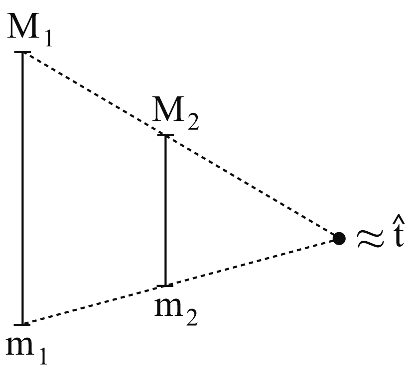
Figure 1: Extrapolation technique given by (14). $M_{1},M_{2}$ and $m_{1},m_{2}$ are the maximum and minimum times respectively, using initial stepsizes $h_{01}$ and $h_{02}$, with $h_{01}>h_{02}$.

In Examples 3 and 4 we do not know the exact value of the blow-up time. However, in order to make a study of the relative error analogous to the previous examples, we have taken as blow-up time for Example 3 the approximation for $h=0.001$ in case 2 with $c_{2}=0.5$: $t=5.78482$; in Example 4 the blow-up time value has been taken as the approximation for $h=0.0001$ in case 2 with $c_{2}=2/3$ (Radau I collocation points): $t=1.645842$. Results are shown in Tables 7, 8, 10 and 11.

The relative error varying $c_{1}$ (case 1) or $c_{2}$ (case 2) is the “relative vertical size” of the graph, and it decreases at the same rate as $h$. On the other hand, the relative error of the intersection decreases faster, in some cases at the same rate as $h^{2}$.

Moreover, in case 1, the best approximations are obtained with $c_{1}\approx 0.5$, and in case 2 with $c_{2}\approx 2/3$ (approximately Radau I) for Examples 1, 2 and 4 (see Tables 3, 6 and 12), while for Example 3 the best approximations are obtained with $c_{2}\approx 0.5$; however, in Table 9 are also shown the approximations and their corresponding errors for the Radau I collocation points. On the other hand, the intersections technique offers better results, but at a greater computational cost.

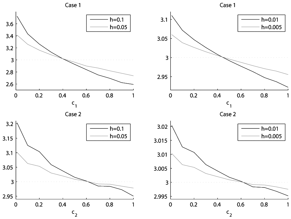
Figure 2: Example 1. Numerical estimation of the blow-up time of collocation solutions varying $c_{1}$ (case 1) or $c_{2}$ (case 2), for different initial stepsizes $h$. The blow-up time of the corresponding (exact) solution is $\hat{t}=3$. The intersection of both curves gives a good approximation of the blow-up time.

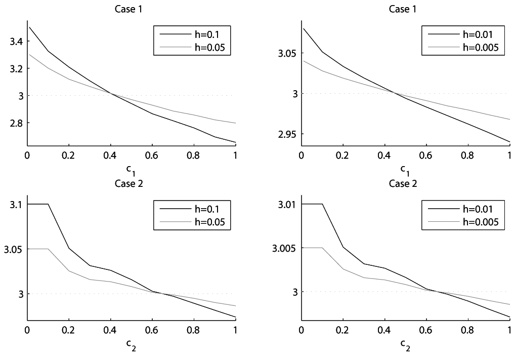
Figure 3: Example 2. Numerical estimation of the blow-up time of collocation solutions varying $c_{1}$ (case 1) or $c_{2}$ (case 2), for different inital stepsizes $h$. The blow-up time of the corresponding (exact) solution is $\hat{t}=3$. The intersection of both curves gives a good approximation of the blow-up time.

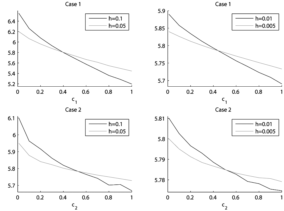
Figure 4: Example 3. Numerical estimation of the blow-up time of collocation solutions varying $c_{1}$ (case 1) or $c_{2}$ (case 2), for different initial stepsizes $h$. The intersection of both curves gives a good approximation of the blow-up time.

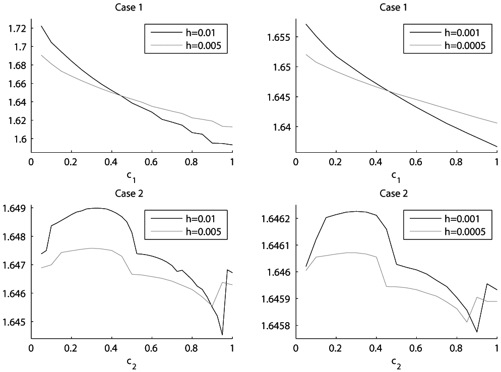
Figure 5: Example 4. Numerical estimation of the blow-up time of collocation solutions varying $c_{1}$ (case 1) or $c_{2}$ (case 2), for different initial stepsizes $h$. The intersection of both curves gives a good approximation of the blow-up time.

5 Discussion and comments

The main necessary conditions for a collocation problem to have a blow-up are obtained from Propositions 3.2 (case 1) and 3.5 (case 2), and are mostly related to the nonlinearity, since the assumption on the kernel “the map $t\mapsto K\left(t,s\right)$ is continuous in $\left]s,\epsilon\right[$ for some $\epsilon>0$ and for all $0\leq s<\epsilon$” is only required in case 2 with $c_{2}\neq 1$ and it is a very weak hypothesis. Hence, assuming that the kernel satisfies this hypothesis, the main necessary condition for the existence of a blow-up is:

• $\frac{y}{G(y)}$ is bounded away from zero.

In addition, for convolution kernels, there is another necessary condition:

• $\frac{G(y)}{y}$ is unbounded away from zero, i.e. there exists a sequence $\left\{y_{n}\right\}_{n=1}^{+\infty}$ of positive real numbers and divergent to $+\infty$ such that $\lim_{n\rightarrow+\infty}\frac{y_{n}}{G\left(y_{n}\right)}=0$.

In [4] it is given a necessary and sufficient condition for the existence of blow-up (exact) solutions for equation (1) with a kernel of the form $K(t,s)=(t-s)^{\alpha-1}r(s)$ with $\alpha>0$, $r$ nondecreasing and continuous for $t\neq 0$, $r(t)=0$ for $t\leq 0$, and $r(t)>0$ for $t>0$:

$$\int_{\delta}^{+\infty}\left(\frac{s}{G(s)}\right)^{1/\alpha}\frac{\textrm{d}s}{s}<+\infty,\qquad\delta>0.$$ (15)

This also holds for convolution kernels of Abel type $K(t,s)=(t-s)^{\alpha-1}$ with $\alpha>0$, generalizing some results given in [3]. Next we will show that necessary conditions 1 and 2 above mentioned are also necessary conditions for the integral given in (15) to be convergent, and thus for the existence of a blow-up (exact) solution.

Proposition 5.1

If (15) holds, then $\frac{G(y)}{y}$ is unbounded away from zero.

Proof.

Let us suppose that $\frac{G(y)}{y}$ is bounded away from zero. So, there exists $M>0$ such that $\frac{G(y)}{y}<M$ for all $y>\delta$. Hence

$$\int_{\delta}^{+\infty}\left(\frac{s}{G(s)}\right)^{1/\alpha}\frac{\textrm{d}s}{s}>\left(\frac{1}{M}\right)^{1/\alpha}\int_{\delta}^{+\infty}\frac{\textrm{d}s}{s}=+\infty.$$

∎

Proposition 5.2

If (15) holds, then $\frac{y}{G(y)}$ is bounded away from zero.

Proof.

By Proposition 5.1, $\frac{G(y)}{y}$ is unbounded away from zero and hence, there exists a strictly increasing sequence $\left\{y_{n}\right\}_{n=1}^{+\infty}$ with $y_{1}>\delta$ and divergent to $+\infty$ such that $\frac{y_{n}}{G\left(y_{n}\right)}<\frac{1}{2^{\alpha}}$ for all $n$.

Let us suppose that $\frac{y}{G(y)}$ is unbounded away from zero; so, we can choose $\left\{y_{n}\right\}_{n=1}^{+\infty}$ such that there exist $y^{\prime}_{n}\in\left]y_{n},y_{n+1}\right[$ with $\frac{y^{\prime}_{n}}{G\left(y^{\prime}_{n}\right)}=1$ for each $n$. Moreover, since $G$ is positive and strictly increasing, we have that $\frac{y^{\prime}_{n}}{G\left(y_{n}\right)}>\frac{y^{\prime}_{n}}{G\left(y^{\prime}_{n}\right)}=1$, and then $y^{\prime}_{n}>G\left(y_{n}\right)$. Hence, we have

$$\int_{y_{n}}^{y_{n+1}}\left(\frac{s}{G(s)}\right)^{1/\alpha}\frac{\textrm{d}s}{s} > \int_{y_{n}}^{y^{\prime}_{n}}\left(\frac{s}{G(s)}\right)^{1/\alpha}\frac{\textrm{d}s}{s}>\int_{y_{n}}^{y^{\prime}_{n}}\left(\frac{s}{G\left(y^{\prime}_{n}\right)}\right)^{1/\alpha}\frac{\textrm{d}s}{s}$$

$$= \alpha\left(1-\left(\frac{y_{n}}{y^{\prime}_{n}}\right)^{1/\alpha}\right)>\alpha\left(1-\left(\frac{y_{n}}{G\left(y_{n}\right)}\right)^{1/\alpha}\right)>\frac{\alpha}{2}.$$

Therefore, (15) does not hold. ∎

The results presented here provide a guide for future research. An interesting problem which is not fully resolved is to determine the relationship between the existence of blow-up in exact solutions and in collocation solutions.

Another open problem is to assure the unboundedness of a collocation solution with adaptive stepsize (in the sense of [9]) using an infinite mesh $I_{h}$ with $\lim_{n\rightarrow\infty}t_{n}<\infty$ in the general case of a non-Lipschitz nonlinearity $G$ (see Remark 4.1). In other words, if we can not arrive at a given time $T$ with any collocation solution (i.e. using any mesh), then, is there a collocation blow-up? If so, and in terms of Definition 4.1, it would be sufficient to hold only the first point for a collocation problem to have a blow-up.

Tables

Case 1	Varying $c_{1}$			Extrapolation		Intersection
$h$	min. $t$	max. $t$	Rel. error	$t$	Rel. error	$t$	Rel. error
$0.1$	$2.60$	$3.66$	$4\cdot 10^{-1}$	$3.033$	$1.1\cdot 10^{-2}$		$10^{-2}$
	($c_{1}=1$)	($c_{1}=0.01$)				$3.03$
$0.05$	$2.78$	$3.40$	$2\cdot 10^{-1}$			($c_{1}=0.39$)
	($c_{1}=1$)	($c_{1}=0.01$)
$0.01$	$2.92$	$3.11$	$6\cdot 10^{-2}$	$3.0044$	$1.5\cdot 10^{-3}$		$7\cdot 10^{-4}$
	($c_{1}=1$)	($c_{1}=0.01$)				$3.002$
$0.005$	$2.96$	$3.06$	$3\cdot 10^{-2}$			($c_{1}=0.44$)
	($c_{1}=1$)	($c_{1}=0.01$)

Table 1: Example 1. Numerical data of Figure 2 (case 1: $m=1$, $c_{1}>0$).

Case 2	Varying $c_{2}$			Extrapolation		Intersection
$h$	min. $t$	max. $t$	Rel. error	$t$	Rel. error	$t$	Rel. error
$0.1$	$2.95$	$3.20$	$8\cdot 10^{-2}$	$3.008$	$2.6\cdot 10^{-3}$		$10^{-4}$
	($c_{2}=1$)	($c_{2}=0.01$)				$3.0003$
$0.05$	$2.98$	$3.10$	$4\cdot 10^{-2}$			($c_{2}=0.618$)
	($c_{2}=1$)	($c_{2}=0.01$)
$0.01$	$2.995$	$3.020$	$8\cdot 10^{-3}$	$3.0008$	$2.6\cdot 10^{-4}$		$10^{-6}$
	($c_{2}=1$)	($c_{2}=0.01$)				$3.000003$
$0.005$	$2.998$	$3.010$	$4\cdot 10^{-3}$			($c_{2}=0.623$)
	($c_{2}=1$)	($c_{2}=0.01$)

Table 2: Example 1. Numerical data of Figure 2 (case 2:$m=2$, $c_{1}=0$).

$h$	Case 1 - $c_{1}=0.5$		Case 2 - Radau I
	Blow-up	Rel. error	Blow-up	Rel. error
$0.1$	$2.933883$	$2.2\cdot 10^{-2}$	$2.995253$	$1.6\cdot 10^{-3}$
$0.05$	$2.965002$	$1.2\cdot 10^{-2}$	$2.997602$	$8\cdot 10^{-4}$
$0.01$	$2.992885$	$2.4q\cdot 10^{-3}$	$2.999519$	$1.6\cdot 10^{-4}$
$0.005$	$2.996434$	$1.2\cdot 10^{-3}$	$2.999759$	$8\cdot 10^{-5}$

Table 3: Example 1. Numerical estimations and relative errors of the blow-up time of collocation solutions in case 1 with $c_{1}=0.5$, and case 2 with Radau I collocation points, $c_{1}=0$, $c_{2}=2/3$, for different initial stepsizes $h$.

Case 1	Varying $c_{1}$			Extrapolation		Intersection
$h$	min. $t$	max. $t$	Rel. error	$t$	Rel. error	$t$	Rel. error
$0.1$	$2.68$	$3.50$	$3\cdot 10^{-1}$	$3.018$	$6\cdot 10^{-3}$		$5\cdot 10^{-3}$
	($c_{1}=1$)	($c_{1}=0.01$)				$3.015$
$0.05$	$2.82$	$3.30$	$1.5\cdot 10^{-1}$			($c_{1}=0.399$)
	($c_{1}=1$)	($c_{1}=0.01$)
$0.01$	$2.94$	$3.08$	$4.6\cdot 10^{-2}$	$3.01$	$3.3\cdot 10^{-3}$		$2.6\cdot 10^{-4}$
	($c_{1}=1$)	($c_{1}=0.01$)				$3.0008$
$0.005$	$2.98$	$3.04$	$2.3\cdot 10^{-2}$			($c_{1}=0.444$)
	($c_{1}=1$)	($c_{1}=0.01$)

Table 4: Example 2. Numerical data of Figure 3 (case 1: $m=1$, $c_{1}>0$).

Case 2	Varying $c_{2}$			Extrapolation		Intersection
$h$	min. $t$	max. $t$	Rel. error	$t$	Rel. error	$t$	Rel. error
$0.1$	$2.97$	$3.10$	$4.3\cdot 10^{-2}$	$3.007$	$2.4\cdot 10^{-3}$		$4\cdot 10^{-5}$
	($c_{2}=1$)	($c_{2}=0.01$)				$3.00012$
$0.05$	$2.99$	$3.05$	$2\cdot 10^{-2}$			($c_{2}=0.6466$)
	($c_{2}=1$)	($c_{2}=0.01$)
$0.01$	$2.997$	$3.010$	$4.3\cdot 10^{-3}$	$3.000003$	$10^{-6}$		$3.6\cdot 10^{-6}$
	($c_{2}=1$)	($c_{2}=0.01$)				$3.000011$
$0.005$	$2.9985$	$3.005$	$2.15\cdot 10^{-3}$			($c_{2}=0.65114$)
	($c_{2}=1$)	($c_{2}=0.01$)

Table 5: Example 2. Numerical data of Figure 3 (case 2: $m=2$, $c_{1}=0$).

$h$	Case 1 - $c_{1}=0.5$		Case 2 - Radau I
	Blow-up	Rel. error	Blow-up	Rel. error
$0.1$	$2.941795$	$2\cdot 10^{-2}$	$2.999559$	$1.5\cdot 10^{-4}$
$0.05$	$2.970341$	$10^{-2}$	$2.999778$	$7.4\cdot 10^{-5}$
$0.01$	$2.993979$	$2\cdot 10^{-3}$	$2.999955$	$1.5\cdot 10^{-5}$
$0.005$	$2.996983$	$10^{-3}$	$2.999978$	$7.3\cdot 10^{-6}$

Table 6: Example 2. Numerical estimations and relative errors of the blow-up time of collocation solutions in case 1 with $c_{1}=0.5$, and case 2 with Radau I collocation points, $c_{1}=0$, $c_{2}=2/3$, for different initial stepsizes $h$.

Case 1	Varying $c_{1}$			Extrapolation		Intersection
$h$	min. $t$	max. $t$	Rel. error	$t$	Rel. error	$t$	Rel. error
$0.1$	$5.20$	$6.55$	$2.3\cdot 10^{-1}$	$5.7625$	$3.8\cdot 10^{-3}$		$3.6\cdot 10^{-3}$
	($c_{1}=1$)	($c_{1}=0.01$)				$5.8055$
$0.05$	$5.45$	$6.20$	$1.3\cdot 10^{-1}$			($c_{1}=0.3961$)
	($c_{1}=1$)	($c_{1}=0.01$)
$0.01$	$5.71$	$5.89$	$3.1\cdot 10^{-2}$	$5.77$	$2.6\cdot 10^{-3}$		$1.4\cdot 10^{-4}$
	($c_{1}=1$)	($c_{1}=0.01$)				$5.7856$
$0.005$	$5.735$	$5.840$	$1.8\cdot 10^{-2}$			($c_{1}=0.441$)
	($c_{1}=1$)	($c_{1}=0.01$)

Table 7: Example 3. Numerical data of Figure 4 (case 1: $m=1$, $c_{1}>0$). The blow-up time of the corresponding (exact) solution is assumed to be $\hat{t}\approx 5.78482$.

Case 2	Varying $c_{2}$			Extrapolation		Intersection
$h$	min. $t$	max. $t$	Rel. error	$t$	Rel. error	$t$	Rel. error
$0.1$	$5.67$	$6.10$	$7.4\cdot 10^{-2}$	$5.793$	$1.4\cdot 10^{-3}$		$3\cdot 10^{-4}$
	($c_{2}=1$)	($c_{2}=0.01$)				$5.78304$
$0.05$	$5.73$	$5.95$	$3.8\cdot 10^{-2}$			($c_{2}=0.5286$)
	($c_{2}=1$)	($c_{2}=0.01$)
$0.01$	$5.775$	$5.810$	$6\cdot 10^{-3}$	$5.785$	$3.1\cdot 10^{-5}$		$3.5\cdot 10^{-6}$
	($c_{2}=1$)	($c_{2}=0.01$)				$5.7848$
$0.005$	$5.779$	$5.800$	$3.6\cdot 10^{-3}$			($c_{2}=0.514$)
	($c_{2}=1$)	($c_{2}=0.01$)

Table 8: Example 3. Numerical data of Figure 4 (case 2: $m=2$, $c_{1}=0$). The blow-up time of the corresponding (exact) solution is assumed to be $\hat{t}\approx 5.78482$.

$h$	Case 1 - $c_{1}=0.5$		Case 2 - Radau I		Case 2 - $c_{2}=0.5$
	Blow-up	Rel. error	Blow-up	Rel. error	Blow-up	Rel. error
$0.1$	$5.694865$	$1.6\cdot 10^{-2}$	$5.751797$	$5.7\cdot 10^{-3}$	$5.788215$	$5.9\cdot 10^{-4}$
$0.05$	$5.739117$	$7.9\cdot 10^{-3}$	$5.767963$	$2.9\cdot 10^{-3}$	$5.786612$	$3.1\cdot 10^{-4}$
$0.01$	$5.775121$	$1.7\cdot 10^{-3}$	$5.781037$	$6.5\cdot 10^{-4}$	$5.784995$	$3\cdot 10^{-5}$
$0.005$	$5.780132$	$8.1\cdot 10^{-4}$	$5.783066$	$3\cdot 10^{-4}$	$5.784875$	$9.5\cdot 10^{-6}$

Table 9: Example 3. Numerical estimations and relative errors of the blow-up time of collocation solutions in case 1 with $c_{1}=0.5$, and case 2 with Radau I collocation points, $c_{1}=0$, $c_{2}=2/3$, and $c_{1}=0$, $c_{2}=0.5$, for different initial stepsizes $h$. The blow-up time of the corresponding (exact) solution is assumed to be $\hat{t}\approx 5.78482$.

Case 1	Varying $c_{1}$			Extrapolation		Intersection
$h$	min. $t$	max. $t$	Rel. error	$t$	Rel. error	$t$	Rel. error
$0.01$	$1.593$	$1.722$	$7.8\cdot 10^{-2}$	$1.6436$	$1.4\cdot 10^{-3}$		$5.2\cdot 10^{-4}$
	($c_{1}=1$)	($c_{1}=0.05$)				$1.6467$
$0.005$	$1.613$	$1.691$	$4.7\cdot 10^{-2}$			($c_{1}=0.444$)
	($c_{1}=1$)	($c_{1}=0.05$)
$0.001$	$1.6367$	$1.6571$	$1.2\cdot 10^{-2}$	$1.6456$	$1.2\cdot 10^{-4}$		$6.6\cdot 10^{-5}$
	($c_{1}=1$)	($c_{1}=0.05$)				$1.64595$
$0.0005$	$1.6406$	$1.6521$	$7\cdot 10^{-3}$			($c_{1}=0.461$)
	($c_{1}=1$)	($c_{1}=0.05$)

Table 10: Example 4. Numerical data of Figure 5 (case 1: $m=1$, $c_{1}>0$). The blow-up time of the corresponding (exact) solution is assumed to be $\hat{t}\approx 1.645842$.

Case 2	Varying $c_{2}$			Extrapolation
$h$	min. $t$	max. $t$	Rel. error	$t$	Rel. error
$0.01$	$1.6445$	$1.6490$	$2.7\cdot 10^{-3}$	$1.64648$	$3.9\cdot 10^{-4}$
	($c_{2}=0.95$)	($c_{2}=0.33$)
$0.005$	$1.6456$	$1.6476$	$1.2\cdot 10^{-3}$
	($c_{2}=0.9$)	($c_{2}=0.3$)
$0.001$	$1.64577$	$1.64622$	$2.7\cdot 10^{-4}$	$1.64586$	$1.4\cdot 10^{-5}$
	($c_{2}=0.9$)	($c_{2}=0.3$)
$0.0005$	$1.64581$	$1.64607$	$1.6\cdot 10^{-4}$
	($c_{2}=0.85$)	($c_{2}=0.28$)

Table 11: Example 4. Numerical data of Figure 5 (case 1: $m=2$, $c_{1}=0$). The intersection method can not be applied because there are more than one intersection. The blow-up time of the corresponding (exact) solution is assumed to be $\hat{t}\approx 1.645842$.

$h$	Case 1 - $c_{1}=0.5$		Case 2 - Radau I
	Blow-up	Rel. error	Blow-up	Rel. error
$0.01$	$1.638700$	$4.3\cdot 10^{-3}$	$1.646991$	$7\cdot 10^{-4}$
$0.005$	$1.642843$	$1.8\cdot 10^{-3}$	$1.646540$	$4.2\cdot 10^{-4}$
$0.001$	$1.645172$	$4.1\cdot 10^{-4}$	$1.645985$	$8.7\cdot 10^{-5}$
$0.0005$	$1.645491$	$2.1\cdot 10^{-4}$	$1.645919$	$4.7\cdot 10^{-5}$

Table 12: Example 4. Numerical estimations and relative errors of the blow-up time of collocation solutions in case 1 with $c_{1}=0.5$, and case 2 with Radau I collocation points, $c_{1}=0$, $c_{2}=2/3$, for different initial stepsizes $h$. The blow-up time of the corresponding (exact) solution is assumed to be $\hat{t}\approx 1.645842$.

References

• [1] C. M. Kirk. Numerical and asymtotic analysis of a localized heat source undergoing periodic motion. Nonlinear Anal. 71 (2009), e2168–e2172.
• [2] F. Calabrò, G. Capobianco. Blowing up behavior for a class of nonlinear VIEs connected with parabolic PDEs. J. Comput. Appl. Math. 228 (2009), 580–588.
• [3] W. Mydlarczyk. A condition for finite blow-up time for a Volterra integral equation. J. Math. Anal. Appl. 181 (1994), 248–253.
• [4] W. Mydlarczyk. The blow-up solutions of integral equations. Colloq. Math. 79 (1999), 147–156.
• [5] T. Małolepszy, W. Okrasiński. Conditions for blow-up of solutions of some nonlinear Volterra integral equations. J. Comput. Appl. Math. 205 (2007), 744–750.
• [6] T. Małolepszy, W. Okrasiński. Blow-up conditions for nonlinear Volterra integral equations with power nonlinearity. Appl. Math. Letters. 21 (2008), 307–312.
• [7] T. Małolepszy, W. Okrasiński. Blow-up time for solutions for some nonlinear Volterra integral equations. J. Math. Anal. Appl. 366 (2010), 372–384.
• [8] H. Brunner. Collocation Methods for Volterra Integral and Related Functional Differential Equations. Cambridge University Press, Cambridge (2004).
• [9] Z. W. Yang, H. Brunner. Blow-up behavior of collocation solutions to Hammerstein-type Volterra integral equations. SIAM J. Numer. Anal. 51 (2013), 2260–2282.
• [10] M. A. Krasnosel’skii, P. P. Zabreiko. Geometric Methods of Nonlinear Analysis. Springer Verlag, New York, 1984.
• [11] R. Benítez, V. J. Bolós. Existence and uniqueness of nontrivial collocation solutions of implicitly linear homogeneous Volterra integral equations. J. Comput. Appl. Math. 235 (2011), 3661–3672.
• [12] H. Brunner. Implicitly linear collocation methods for nonlinear Volterra integral equations. Appl. Numer. Math. 9 (1992), 235–247.
• [13] M.R. Arias, R. Benítez, Aspects of the behaviour of solutions of nonlinear Abel equations. Nonlinear Anal. T.M.A., 54 (2003), pp. 1241–1249.
• [14] M.R. Arias, R. Benítez, A note of the uniqueness and the attractive behaviour of solutions for nonlinear Volterra equations, J. Integral Equations Appl. 13 (4) (2001) 305–310.