Relaxation at finite temperature in Fully-Frustrated Ising Models

Abstract

We consider by means of Monte Carlo simulations the relaxation in the paramagnetic phase of the anti-ferromagnetic Ising model on a triangular lattice and of a fully-frustrated Ising model on a square lattice. In contradistinction to previous studies of the second model, we show that spin-spin correlation functions do not decay with a stretched-exponential law at low temperature but that both models display an exponential decay with logarithmic corrections that are interpreted as the signature of topological defects.

1 Introduction

The study of relaxation in frustrated systems is of particular interest because their dynamics may become anomalously slow at low temperature and eventually freeze below a certain temperature. The paradigmatic example of such a slow dynamics is given by spin glasses which combine both frustration and randomness. Frustration alone does not necessarily imply a glassy dynamics. Even though each one of its plaquettes is frustrated, the anti-ferromagnetic Ising model on a triangular lattice [14] (AFIM) was shown to display the same dynamics as unfrustrated systems [17]. Interestingly, if elastic deformations of the lattice are allowed and coupled to the spin degrees of freedom, the relaxation is well described by a (stretched-exponential) Kohlrausch-Williams-Watts law like in glasses [1, 6, 15]. This behavior is observed experimentally for example with closely-packed colloidal spheres [7].

In this paper, we consider both the AFIM and the Fully-Frustrated Ising Model (FFIM) defined on a square lattice by the Hamiltonian

$$-\beta H=\sum_{x,y}\big{[}\sigma_{x,y}\sigma_{x+1,y}+(-1)^{f(x,y)}\sigma_{x,y}\sigma_{x,y+1}\big{]},\quad\quad\sigma_{x,y}=\pm 1$$ (1)

where $f(x,y)=x+y$ in the so-called zigzag model and $f(x,y)=x$ in pileup-domino configuration. In both cases, each plaquette of the square lattice contains an odd number of anti-ferromagnetic bonds and, as a consequence, is frustrated. The pileup-domino configuration allows for exact diagonalization of the transfer matrix by free fermion techniques [12]. Both AFIM and FFIM are known to belong to the same universality class. At the critical temperature $T_{c}=0$, spin-spin autocorrelation functions decay algebraically

$$C(t,s)=\langle\sigma(t)\sigma(s)\rangle\sim(t-s)^{-\eta/z}$$ (2)

where $\eta=1/2$ and $z=2$ is the dynamical exponent. In the case of the AFIM, evidences have been given of the existence of topological defects interacting through a logarithmic Coulombian potential in the paramagnetic phase [11, 16]. While no signature of these defects was observed in earlier simulations of the AFIM [9], we have shown that such defects manifest themselves in the FFIM [13]. When the system is initially prepared in the paramagnetic phase and then quenched at $T_{c}=0$, they pin the domain walls and slow down their motion so that aging takes place in the same way as in homogeneous systems but with logarithmic corrections. The correlation length grows as $\xi(t)\sim(t/\ln t)^{1/z}$ and spin-spin autocorrelation functions behave as

$$C(t,s)\sim s^{-\eta/z}\left({t\ln s\over s\ln t}\right)^{-\lambda/z}$$ (3)

where both $z$ and $\lambda$ are compatible with $2$.

This result suggests that at finite temperature, the relaxation should be exponential, like in unfrustrated systems, but with logarithmic corrections due to the presence of topological defects. However, on the basis of Monte Carlo simulations, a stretched-exponential relaxation 

$$C(t)\sim e^{-(t/\tau)^{\kappa}}$$ (4)

with a temperature-dependent exponent $\kappa$ has been reported in the FFIM below the temperature $T_{p}\simeq 1.701$ at which Kasteleyn-Fortuin clusters start to percolate [2, 4]. In this work, we reconsider the AFIM and the FFIM and show that Monte Carlo data are in better agreement with an exponential decay when taking into account logarithmic corrections than with a stretched exponential. In the first section, a dynamical scaling hypothesis is set up to predict the behavior of equilibrium spin-spin autocorrelation functions in fully-frustrated Ising models. The expression is then compared with Monte Carlo data for the AFIM in the second section and the FFIM in the third one.

2 Dynamical scaling of spin-spin autocorrelation functions

We analyze the two-time spin-spin correlation functions in the framework of dynamical scaling [8]. Upon a dilatation with a scale factor $b$, the equilibrium correlation $C(\vec{r},t,T)=\langle\sigma_{0}(0)\sigma_{\vec{r}}(t)\rangle$ at temperature $T$ is assumed to satisfy the homogeneity relation

$$C(\vec{r},1/t,|T-T_{c}|)=b^{-2x_{\sigma}}C\big{(}r/b,b^{z}/t,|T-T_{c}|b^{1/\nu}\big{)}$$ (5)

where $x_{\sigma}$ is the scaling dimension of magnetization density with $2x_{\sigma}=\eta$ for two-dimensional systems and $z$ is the dynamical exponent. The motivation for the last two arguments of the scaling function in equation (5) comes for the behavior of the correlation length either with time, $\xi\sim t^{1/z}$, or with temperature, $\xi\sim|T-T_{c}|^{-1/\nu}$. Letting $b=t^{1/z}$ in equation (5), we obtain

$$C(\vec{r},t)=t^{-\eta/z}{\cal C}\big{(}r/t^{1/z},|T-T_{c}|t^{1/\nu z}\big{)}$$ (6)

The algebraic prefactor corresponds to the critical behavior while the scaling function includes all corrections to it. The characteristic time

$$\tau\sim\xi^{z}\sim|T-T_{c}|^{-\nu z}$$ (7)

appears as the relaxation time of the system. In the following, we are interested only in autocorrelation functions, i.e. $r=0$. Moreover, we expect an exponential decay of the scaling function ${\cal C}(t/\tau)$ in the paramagnetic phase. Therefore, the autocorrelation function generally reads at equilibrium

$$C(t,T)\sim{e^{-t/\tau}\over t^{\eta/z}}$$ (8)

Two modifications need to be made to apply this hypothesis to the AFIM and the FFIM. First, as already mentioned, the existence of topological defects slows down the motion of domain walls and thus the growth of the correlation length, i.e. $\xi\sim(t/\ln t)^{1/z}$. A logarithmic correction has to be included in the scaling hypothesis (6)

$$C(0,t)=t^{-\eta/z}{\cal C}\big{(}0,|T-T_{c}|(t/\ln t)^{1/\nu z}\big{)}\sim{e^{-t/\tau\ln t}\over t^{\eta/z}}$$ (9)

The algebraic decay in front of the scaling function is not affected by logarithmic corrections because it describes the critical behavior for which topological defects are paired. In contradistinction, the scaling function ${\cal C}$ corresponds to the deviation to this behavior caused by non-vanishing scaling fields. The latter brings the system out-of-criticality, i.e. into the paramagnetic phase where free topological defects are encountered. ${\cal C}$ should thus involve logarithmic corrections. Note that the same kind of behavior was assumed during aging (3). The second modification concerns the relaxation time. Since the correlation length is known [3, 10] to diverge exponentially with temperature, i.e. $\xi\sim e^{2/T}$ and not algebraically, equation (7) has to be replaced by

$$\tau\sim\xi^{z}\sim e^{2z/T}.$$ (10)

3 Relaxation of the AFIM

We have studied the AFIM and FFIM by means of large-scale Monte Carlo simulations for a two-dimensional lattice with $192\times 192$ sites. The dynamics is the heat-bath local Markovian process introduced by Glauber [5]. We shall consider first the AFIM. Inverse temperatures $\beta=1/k_{B}T$ in the range $[0.75;3.00]$ have been considered. Data have been averaged over $30,000$ independent histories. Error bars on the average correlation $C(t,s)$ have been estimated at each times $t$ and $s$ as the standard deviation of the data produced during the different independent histories.

To check that the system had thermalized when the measurements were started, we monitored the two-time spin-sin correlation functions $C(t,s)$ which are expected to depend only on $t-s$ in the stationary state. On figure 1, spin-spin autocorrelation functions of the AFIM are plotted at different temperatures with respect to $t-s$. For sufficiently large values of $s$, one can observe the collapse of the curves, indicating that the system has reached equilibrium. In the example of the data presented in figure 1, one is led to the conclusion that below the inverse temperature $\beta=1/k_{B}T=1.75$, equilibrium has already been reached at time $s=1000$. At $\beta=1.75$, equilibrium is reached only at time $s=2000$ while for larger values of $\beta$, no collapse is observed indicating that equilibrium is not reached yet at time $s=4500$. For this reason, only inverse temperatures $\beta\leq 1.75$ with $s\geq 2000$ will be considered in the following.

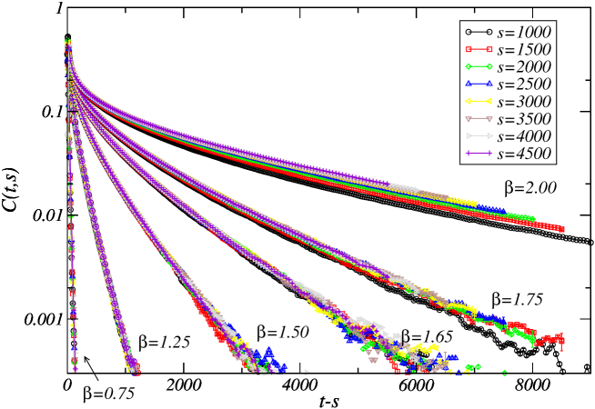
Figure 1: Relaxation of the spin-spin correlation function $C(t,s)$ of the AFIM versus $t-s$ at six different inverse temperatures $\beta=0.75$, $1.25$, $1.50$, $1.65$, $1.75$, and $2.00$. The different curves correspond to different times $s$. Error bars are represented but they are hardly visible on the figure because they are of order ${\cal O}(10^{-5})$, i.e. much smaller than the symbols.

We have tested three possible scenarii: exponential decay of the spin-spin autocorrelation functions (8), exponential decay with logarithmic corrections (9), and stretched exponential (4). On figure 2, the scaling function $C(t,s)(t-s)^{1/4}$ is plotted versus $t-s$ with a waiting time $s=2000$ (ensuring equilibration as discussed above). In the scenario (8), this function is expected to decay exponentially. This behavior is indeed observed over a large range of times $t-s$ for all inverse temperatures $\beta\leq 1.75$. We estimated the relaxation time by interpolation of the scaling function as $e^{-t/\tau}$ with a sliding interpolation window. As can be seen in the inset of figure 2, the dependence of $\tau$ on $\beta$ is well described by an exponential, as expected for the AFIM (see equation 10). A fit gives $\tau\sim e^{4.31(2)\beta}$, a behavior which is close to the expected one (10), thought significantly outside error bars.

Figure 2: Scaling function $C(t,s)(t-s)^{1/4}$ at time $s=2000$ versus $t-s$ for the AFIM at different inverse temperatures $\beta=0.75$, $1.25$, $1.50$, $1.65$, and $1.75$ (from left to right). In the inset, the relaxation time $\tau$ obtained by interpolation of the scaling function as $e^{-(t-s)/\tau}$ is plotted versus the inverse temperature $\beta$. The straight line is the interpolated behavior $\tau\sim e^{4.31(2)\beta}$.

On figure 3, the second scenario (9) is tested. The scaling function $C(t,s)(t-s)^{1/4}$ is plotted versus $(t-s)/\ln(t-s)$. The interpolation with an exponential gives the values represented in the inset. As before, the relaxation time behaves exponentially with the inverse temperature. A fit gives the law $\tau\sim e^{3.92(2)\beta}$, a behavior which is much closer to (10) than without logarithmic corrections, even though still outside error bars.

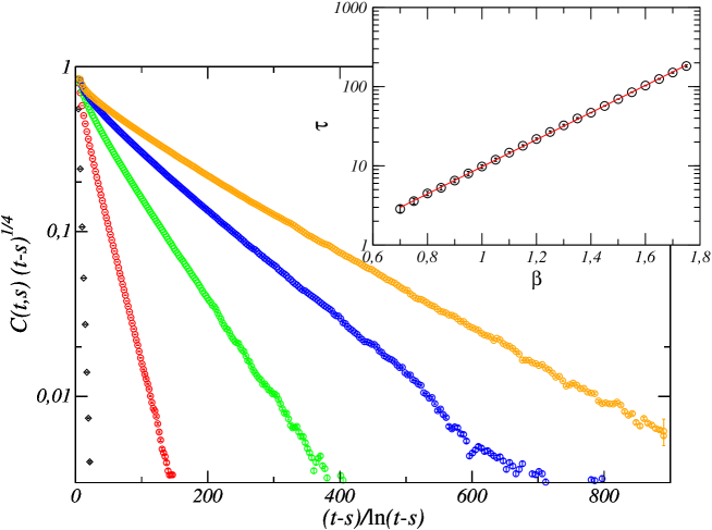
Figure 3: Scaling function $C(t,s)(t-s)^{1/4}$ at time $s=2000$ versus $(t-s)/\ln(t-s)$ for the AFIM at different inverse temperatures $\beta=0.75$, $1.25$, $1.50$, $1.65$, and $1.75$ (from from left to right). In the inset, the relaxation time $\tau$ obtained by interpolation of the scaling function as $e^{-(t-s)/\tau\ln(t-s)}$ is plotted versus the inverse temperature $\beta$. The straight line is the interpolated behavior $\tau\sim e^{3.92(2)\beta}$.

Finally, the stretched exponential scenario is tested on figure 4. The expected power-law behavior in the long-time regime (according to equation 4) is observed only for a narrow interval of times, much narrower than in the two previous scenarii. We have nevertheless interpolated the data with equation (4) to extract the relaxation time. The result is plotted in the inset of figure 4. An exponential growth is observed but with a quite different factor: $\tau\sim e^{2.79(2)\beta}$.

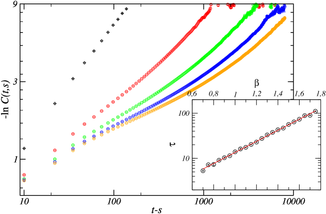
Figure 4: Scaling function $-\ln C(t,s)$ at time $s=2000$ versus $t-s$ for the AFIM at different inverse temperatures $\beta=0.75$, $1.25$, $1.50$, $1.65$ and $1.75$ (from top to bottom). In the inset, the relaxation time $\tau$ obtained by interpolation of the correlation function as $e^{-\big{(}{t-s\over\tau}\big{)}^{\kappa}}$ is plotted versus the inverse temperature $\beta$. The straight line is the interpolated behavior $\tau\sim e^{2.79(2)\beta}$.

4 Relaxation of the FFIM

The FFIM has been studied in the zig-zag bond configuration for a $192\times 192$ square lattice. We restricted ourselves to inverse temperatures smaller or equal to $\beta=1$. As a consequence, smaller times and fewer histories were necessary. Monte Carlo data have been averaged over $1,000$ independent histories. On figure 5, spin-spin autocorrelation functions $C(t,s)$ are presented for different temperatures. The collapse of the different curves indicates that thermalization is achieved very rapidly. Like for the AFIM, we have compared the three scenarii: exponential decay of the spin-spin autocorrelation functions (8), exponential decay with logarithmic corrections (9), and stretched exponential (4).

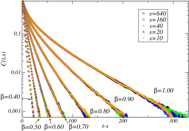
Figure 5: Relaxation of the spin-spin correlation function $C(t,s)$ of the FFIM versus $t-s$ at six different inverse temperatures $\beta=0.50$, $0.60$, $0.70$, $0.80$, $0.90$ and $1.00$. The different colors correspond to different times $s$ as indicated in the legend.

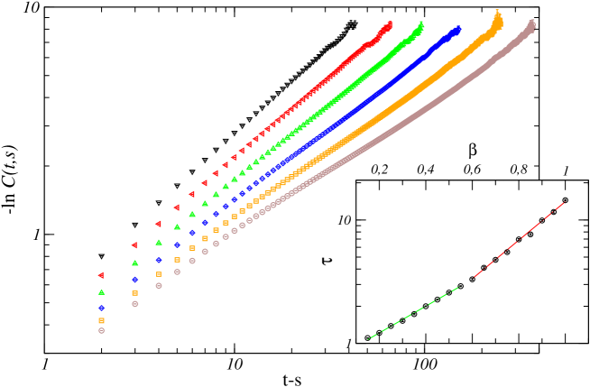
Figure 6: Logarithm $-\ln C(t,s)$ of the spin-spin correlation of the FFIM at different inverse temperatures $\beta=0.50$, $0.60$, $0.70$, $0.80$, $0.90$, and $1.00$ (from top to bottom). Only the time $s=160$ is presented. In the inset, the relaxation time $\tau$ obtained by interpolation of the correlation function as $e^{-\big{(}{t-s\over\tau}\big{)}^{\kappa}}$ is plotted versus the inverse temperature $\beta$. The two straight lines are the interpolated behaviors $\tau\sim e^{3.60(5)\beta}$ for $\beta\geq 0.6$ and $\tau\sim e^{2.50(2)\beta}$ for $\beta<0.6$.

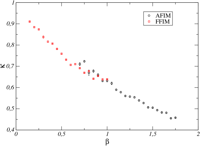
Figure 7: Exponent $\kappa$ of the stretched exponential versus the inverse temperature $\beta$ for both the AFIM (black) and the FFIM (red).

First, we present the test of the stretched-exponential scenario for the FFIM (figure 6). The logarithm $-\ln C(t,s)$ displays a behavior similar to the AFIM. At first sight, the power-law behavior that is expected according to equation (4) seems to be observed over a larger range of times $t-s$ than for the AFIM but one should keep in mind that the inverse temperatures are different on figures 4 and 6. We have estimated the exponent $\kappa$ of the stretched exponential. Our data confirm the general trend observed in references [2, 4]. The exponent $\kappa$ indeed strongly depends on the temperature. However, we do not recover a purely exponential decay above the percolation temperature of the Fortuin-Kasteleyn clusters. We do not observe two regimes ($\kappa=1$ for $T>T_{p}$ and $\kappa$ decreasing below $T_{p}$) as previously found but instead, an exponent slowly approaching a value $\kappa=1$ (see figure 7). The discrepancy may be explained by the larger lattice size used in this study ($L=192$ instead of $L=64$) and by the difficulty to identify a sufficiently large power-law regime, especially at low temperature. As shown in the inset of figure 6, the relaxation time $\tau$ does grow exponentially over the whole range of inverse temperatures $\beta$ considered, in contradistinction to the theoretical prediction (10). However, our data are compatible with two distinct regimes of exponential growth with a prefactor estimated to be $3.60(5)$ for $\beta\geq 0.6$ and $2.50(2)$ for $\beta<0.6$ (note that $\beta_{t}\simeq 0.59$).

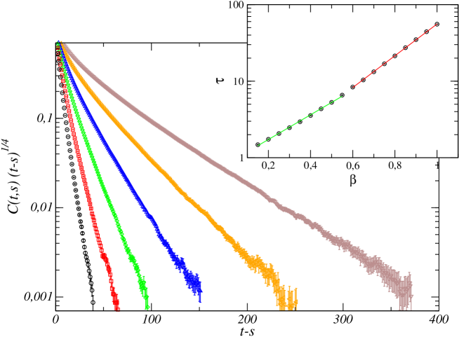
Figure 8: Scaling function $C(t,s)(t-s)^{1/4}$ at time $s=160$ versus $t-s$ for the FFIM at different inverse temperatures $\beta=0.50$, $0.60$, $0.70$, $0.80$, $0.90$, and $1.00$ (from left to right). In the inset, the relaxation time $\tau$ obtained by interpolation of the scaling function as $e^{-(t-s)/\tau}$ is plotted versus the inverse temperature $\beta$. The two straight lines are the interpolated behaviors $\tau\sim e^{4.78(2)\beta}$ for $\beta\geq 0.6$ and $\tau\sim e^{3.72(5)\beta}$ for $\beta<0.6$.

On figure 8, the second scenario is tested. As expected, the scaling function $C(t,s)(t-s)^{1/4}$ displays an exponential decay with $t-s$ over a large range of times $t-s$ for different temperatures. However, the relaxation time does not grow exponentially over the whole range of temperatures considered (inset of figure 8). Again, two regimes can be distinguished: the prefactor in the exponential (10) is estimated to be $4.78(2)$ for $\beta\geq 0.6$ and $3.72(5)$ for $\beta<0.6$. These values should be compared with the theoretical prediction $4$.

On figure 9, the third scenario involving logarithmic corrections is tested. The scaling function $C(t,s)(t-s)^{1/4}$ decay exponentially with $(t-s)/\ln(t-s)$ over a large range of times $t-s$ for different temperatures. The relaxation time $\tau$ now displays an exponential growth over the whole range of temperatures considered and our estimate $4.097(26)$ of the prefactor in the argument of the exponential is much closer to the theoretical prediction $4$ according to equation (10) than without logarithmic corrections.

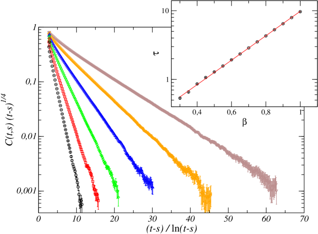
Figure 9: Scaling function $C(t,s)(t-s)^{1/4}$ at time $s=1600$ versus $(t-s)/\ln(t-s)$ for the AFIM at different inverse temperatures $\beta=0.50$, $0.60$, $0.70$, $0.80$, $0.90$, and $1.00$ (from bottom to top). In the inset, the relaxation time $\tau$ obtained by interpolation of the scaling function as $e^{-(t-s)/\tau\ln(t-s)}$ is plotted versus the inverse temperature $\beta$. The straight line is the interpolated behavior $\tau\sim e^{4.097(26)\beta}$.

Model	Stretched exponential	Exponential	Log. corrections
AFIM	$2.79(2)$	$4.31(2)$	$3.92(2)$
FFIM	$3.60(5)$ ($\beta\geq 0.6$)	$4.78(2)$ ($\beta\geq 0.6$)	$4.097(26)$

Table 1: Prefactor in the argument of the exponential growth (10) of the relaxation time for the two models AFIM and FFIM in the different studied scenarii. The theoretical prediction is $4$.

5 Conclusions

We have analyzed the decay of the equilibrium two-time spin-spin correlation functions in the paramagnetic phase against three scenarii: exponential decay of the spin-spin autocorrelation functions (8), exponential decay with logarithmic corrections (9), and stretched exponential (4). To distinguish between them, we tested the thermal behavior (10) of the relaxation time in the different scenarii. Our results are summarized in table 1. The best agreement with the theoretical prediction $4$ is obtained with an exponential decay with logarithmic corrections (9) for both the AFIM and the FFIM. Error bars are unfortunately smaller than the deviation from the theoretical prediction. A great care has been taken in the computation of error bars (from the data production to the analysis) so we can only invoke finite-size effects or other systematic deviations. The deviation for the two other scenarii being much larger, we do not expect them to get closer to $4$ than the exponential decay with logarithmic corrections. These results bring further evidences of the existence of topological defects in the paramagnetic phase of the AFIM and the FFIM.

References

References

- [1] Z. Chen and M. Kardar. Elastic antiferromagnets on a triangular lattice. Journal of Physics C: Solid State Physics, 19:6825–6831, 1986.
- [2] A. Fierro, G. Franzese, A. de Candia, and A. Coniglio. Percolation transition and the onset of nonexponential relaxation in fully frustrated models. Physical Review E, 59:60, 1999.
- [3] G. Forgacs. Ground-state correlations and universality in two-dimensional fully frustrated systems. Physical Review B, 22:4473–4480, 1980.
- [4] G. Franzese and A. Coniglio. Precursor phenomena in frustrated systems. Physical Review E, 59:6409–6412, 1999.
- [5] R. J. Glauber. Time-Dependent statistics of the ising model. Journal of Mathematical Physics, 4:294, 1963.
- [6] L. Gu, B. Chakraborty, P. L. Garrido, M. Phani, and J. L. Lebowitz. Monte carlo study of a compressible ising antiferromagnet on a triangular lattice. Physical Review B, 53:11985, 1996.
- [7] Y. Han, Y. Shokef, A. M. Alsayed, P. Yunker, T. C. Lubensky, and A. G. Yodh. Geometric frustration in buckled colloidal monolayers. Nature, 456:898–903, 2008.
- [8] P. C. Hohenberg and B. I. Halperin. Theory of dynamic critical phenomena. Reviews of Modern Physics, 49:435, 1977.
- [9] E. Kim, B. Kim, and S. J. Lee. Nonequilibrium critical dynamics of the triangular antiferromagnetic ising model. Physical Review E, 68:066127, 2003.
- [10] J. Lukic, E. Marinari, and O. C. Martin. Finite-size scaling in villain’s fully frustrated model and singular effects of plaquette disorder. Europhysics Letters (EPL), 73:779–785, 2006.
- [11] C. Moore, M. G. Nordahl, N. Minar, and C. R. Shalizi. Vortex dynamics and entropic forces in antiferromagnets and antiferromagnetic potts models. Physical Review E, 60:5344–5351, 1999.
- [12] J. Villain. Spin glass with non-random interactions. Journal of Physics C: Solid State Physics, 10:1717–1734, 1977.
- [13] J.-C. Walter and C. Chatelain. Logarithmic corrections in the ageing of the fully frustrated ising model. Journal of Statistical Mechanics: Theory and Experiment, 2008:P07005, 2008.
- [14] G. H. Wannier. Antiferromagnetism. the triangular ising net. Phys. Rev. B, 7:5017–5017, 1973.
- [15] H. Yin and B. Chakraborty. Slow dynamics and aging in a nonrandomly frustrated spin system. Physical Review E, 65:036119, 2002.
- [16] H. Yin, B. Chakraborty, and N. Gross. Effective field theory of the zero-temperature triangular-lattice antiferromagnet: A monte carlo study. Physical Review E, 61:6426–6433, 2000.
- [17] C. Zeng and C. L. Henley. Zero-temperature phase transitions of an antiferromagnetic ising model of general spin on a triangular lattice. Physical Review B, 55:14935–14947, 1997.