Measurement of halo properties with weak lensing shear and flexion

Abstract

We constrain properties of cluster haloes by performing likelihood analysis using lensing shear and flexion data. We test our analysis using two mock cluster haloes: an isothermal ellipsoid (SIE) model and a more realistic elliptical Navarro-Frenk-White (eNFW) model. For both haloes, we find that flexion is more sensitive to the halo ellipticity than shear. The introduction of flexion information significantly improves the constraints on halo ellipticity, orientation and mass. We also point out that there is a degeneracy between the mass and the ellipticity of SIE models in the lensing signal.

1 Introduction

The properties of galaxy and cluster haloes are of great interest in cosmology, and can be powerful tests of the cosmological paradigm and the nature of dark matter. Two important parameters that describe a dark matter halo are its mass and shape, which are related to many physical processes, such as the growth and merging history (Kauffmann et al. 1993; Springel et al. 2005).

Models of dark matter haloes beyond the spherical approximation are favored by many numerical simulations (Jing & Suto 2002; Springel et al. 2004; Kazantzidis et al. 2004; Allgood et al. 2006) and observations (Reblinsky 2000; Lee & Suto 2004; De Filippis et al. 2005; Sereno et al. 2006; Wang et al. 2010). Furthermore, numerical simulations with different assumptions predict different properties of dark matter haloes (e.g. Bullock 2002; Bailin & Steinmetz 2005; Wang & White 2007). Current models based on N-body simulations, semi-analytic models or hydrodynamic simulations can predict several halo properties, but several ingredients of these models remain uncertain. A precise understanding of halo properties such as mass and ellipticity is important to confirm and improve the existing models of galaxy formation and probe the physical nature of dark matter.

Gravitational lensing is a powerful tool to study mass distributions, independent of the nature or dynamical state of the matter (see Mellier 1999; Schneider 2006; Munshi et al. 2008, for reviews). Galaxy-Galaxy Lensing (GGL) is concerned with the mass associated with galaxies and dark matter haloes in which galaxies reside (Tyson et al. 1984; Brainerd et al. 1996; Hudson et al. 1998; Hoekstra et al. 2004; Sheldon et al. 2004; Mandelbaum et al. 2006). The distortion caused by a single galaxy cannot be detected, but the statistics of many foreground-background pairs yield a detectable signal for a population of galaxies. Brainerd et al. (1996) discovered a significant GGL shear signal. Schneider & Rix (1997) developed a maximum likelihood analysis that can constrain the halo properties of the lens galaxy populations through GGL, allowing to estimate the mean velocity dispersion and the characteristic scale for a non-singular isothermal sphere halo model.

Flexion as the gradient of the projected mass density, is sensitive to the small-scale variations of mass distributions (Goldberg & Natarajan 2002; Goldberg & Bacon 2005; Bacon et al. 2006). Different techniques have been developed to measure flexion (see Irwin & Shmakova 2006; Okura et al. 2007; Schneider & Er 2008; Fluke & Lasky 2011, for examples). Recently, Velander et al. (2011) applied the shapelets technique on the COSMOS survey, and Cain et al. (2011) introduced a new method (so-called analytic image model) to analyse lensing flexion images. It has been noted that flexion can contribute to cosmology in several aspects, such as exploring the mass distribution of dark matter haloes of galaxies and clusters, especially substructures (Leonard et al. 2009; Bacon et al. 2010; Er et al. 2010). Hilbert et al. (2011) also propose to reduce the distance measurement errors of standard candles using lensing shear and flexion maps.

In Hawken & Bridle (2009); Er & Schneider (2011); Er et al. (2011), the ellipticity of a galaxy halo has been studied with flexion. It was found that the constraints from flexion are tighter than those from shear. In Goldberg & Bacon (2005), Galaxy-Galaxy lensing Flexion (GGF) has been studied using the distribution function of orientations between the line connecting foreground and background pairs and the flexion of the background galaxies. A GGF signal has been detected by Leonard et al. (2007) using images taken by HST ACS in the cluster Abell 1689. Moreover, combining shear and flexion information provides tighter constraints on halo properties by studying mass distribution on different scales (Er et al. 2010; Shapiro et al. 2010; Hilbert et al. 2011).

In this paper, we combine shear and flexion data to constrain the properties of dark matter haloes. The tangential shear is mainly sensitive to the mass of the halo, whereas flexion is sensitive to the halo ellipticity. Moreover the usable number density of flexion data is relatively low, since the flexion signal drops faster than the shear signal with the angular distance to the centre of the halo. It is thus not sufficient to constrain the halo properties with shear or flexion alone. Therefore, we propose to take advantage of both shear and flexion in our analysis. In particular, we use the angular positions, tangential shear and flexion of galaxies in our likelihood functions. A singular isothermal ellipsoid model and an elliptical NFW model for a galaxy or cluster halo with 3 parameters (mass, ellipticity and orientation) are adopted in this paper. In Sec. 2, we recall the basic lensing equations. Our likelihood function is introduced in Sec. 3. We perform numerical tests of our method and results in Sec. 4 and present our conclusions in Sec. 5. Throughout this paper, we adopt a $\Lambda$CDM model with $\Omega_{\Lambda}=0.75$, $\Omega_{\rm m}=0.25$, and a Hubble constant $H_{0}=73$ km s^-1 Mpc^-1.

2 Lensing Basics

The formalism described here can be found in Schneider & Er (2008); Er & Schneider (2011). The weak lensing shear and flexion are conveniently described using a complex formalism. We adopt the thin lens approximation, assuming that the lensing mass distribution is projected onto a single lens plane. The dimensionless projected mass density can be written as $\kappa(\mbox{\boldmath$\theta$})=\Sigma(\mbox{\boldmath$\theta$})/\Sigma_{\rm cr}$, where $\theta$ is the vector of (angular) position coordinates, $\Sigma(\mbox{\boldmath$\theta$})$ is the projected mass density and $\Sigma_{\rm cr}$ is the critical density, given by

$$\Sigma_{\rm cr}={c^{2}\over 4\pi G}{D_{\rm s}(\infty)\over D_{\rm d}D_{\rm d,\infty}},$$ (1)

for a fiducial source located at a redshift $z\to\infty$. Here $D_{\rm s}(\infty)$, $D_{\rm d}$ and $D_{\rm d,\infty}$ are the angular diameter distances between the observer and the source, the observer and the lens and between the lens and the source, respectively.

The first order image distortion induced by gravitational lensing is the shear $\gamma$, which transforms a circular source into an elliptical one. The second order effect, called flexion, is described by two parameters: the spin-1 flexion, which is the complex derivative of $\kappa$

$${\cal F}=\nabla_{\rm c}\kappa={\partial\kappa\over\partial\theta_{1}}+{\rm i}{\partial\kappa\over\partial\theta_{2}},$$ (2)

and the spin-3 flexion, which is the complex derivative of $\gamma$

$${\cal G}=\nabla_{\rm c}\gamma.$$ (3)

For a source at redshift $z_{\rm s}$ and a lens at redshift $z_{\rm d}$, a ‘cosmological weight’ function must be introduced:

$$Z(z_{\rm s})\equiv\left[D_{\rm d,\infty}\over D_{\infty}\right]^{-1}{D_{\rm ds}\over D_{\rm s}}\,H(z_{\rm s}-z_{\rm d}),$$ (4)

where $D_{\rm ds}$ and $D_{\rm s}$ are the angular diameter distances between the lens and the source, and the observer and the source. $H(z_{\rm s}-z_{\rm d})$ is the Heaviside step function to ensure that the source redshift is higher than the lens redshift. The first and second-order lensing effects scale with the source redshift as

$$\kappa(z_{\rm s})=Z(z_{\rm s})\kappa, \gamma(z_{\rm s})=Z(z_{\rm s})\gamma,$$

$${\cal F}(z_{\rm s})=Z(z_{\rm s}){\cal F}, {\cal G}(z_{\rm s})=Z(z_{\rm s}){\cal G}.$$ (5)

In GGL we express the shear with respect to a foreground halo. This defines the tangential shear

$$\gamma_{\rm t}=-\gamma_{1}\cos 2\psi-\gamma_{2}\sin 2\psi,$$ (6)

where $\gamma_{1}$, $\gamma_{2}$ are respectively the real and the imaginary components of shear, and $\psi$ is the polar angle with respect to the vector connecting the background and foreground galaxies. ${\cal F}_{1}$ (${\cal G}_{1}$) and ${\cal F}_{2}$ (${\cal G}_{2}$) are the real and imaginary components of the spin-1 (spin-3) flexion.

In this paper, $\gamma_{\rm t}$, ${\cal F}_{1}$, ${\cal F}_{2}$, ${\cal G}_{1}$ and ${\cal G}_{2}$ represent the values calculated from our model, while $e$, ${\cal F}^{\rm obs}_{1}$, ${\cal F}^{\rm obs}_{2}$, ${\cal G}^{\rm obs}_{1}$ and ${\cal G}^{\rm obs}_{2}$ are the observables, which will be introduced in the next section.

3 Methodology

We apply the Bayesian framework to study galaxy-galaxy lensing simulated maps, in order to estimate physical parameters of a foreground dark matter halo. The maps contain tangential shear and two flexion components at the positions of background galaxies. The values of these observables reflect the intrinsic shapes of the background images, slightly modified by lensing due to the gravitational potential of a foreground halo.

We assume the shear and flexion components can be measured with unbiased estimators that are linear combinations of the lensing and intrinsic contributions to an image shape. The ellipticity of background galaxies $e$ is such an estimator. Analogously, we assume that the estimators of flexion, ${\cal F}^{\rm obs}_{1}$, ${\cal F}^{\rm obs}_{2}$, ${\cal G}^{\rm obs}_{1}$ and ${\cal G}^{\rm obs}_{2}$ are derived from higher-order brightness moments of the background images. We further assume that the noise of such estimators is uncorrelated due to the distributions of intrinsic shapes, and neglect other contributions, such as sample variance.

The intrinsic ellipticity distribution can be described by a Gaussian probability density distribution with zero mean and standard deviation $\sigma_{e}\approx 0.3$ (Brainerd et al. 1996). For flexion, we use the preliminary studies of intrinsic flexion by Goldberg & Bacon (2005) and Goldberg & Leonard (2007), where scatter of $\sigma_{\cal F}=0.03$ per arcsecond and $\sigma_{\cal G}=0.04$ per arcsecond were found for spin-1 and spin-3 flexion, respectively. In this paper, we also assume that the distribution of each intrinsic flexion noise component $n_{Fj}={\cal F}^{\rm obs}_{j}-{\cal F}_{j}$, $n_{Gj}={\cal G}^{\rm obs}_{j}-{\cal G}_{j}$ ($j=1,2$) is a Gaussian with zero mean and $\sigma_{\cal F}=0.03/^{\prime\prime}$, $\sigma_{\cal G}=0.04/^{\prime\prime}$

$$P(n_{Fj})={1\over\sqrt{2\pi}\sigma_{\cal F}}{\rm exp}\left[-\frac{n_{Fj}^{2}}{2\sigma_{\cal F}^{2}}\right]\,,$$ (7)

$$P(n_{Gj})={1\over\sqrt{2\pi}\sigma_{\cal G}}{\rm exp}\left[-\frac{n_{Gj}^{2}}{2\sigma_{\cal G}^{2}}\right]\,.$$ (8)

Constraints on the foreground haloes parameters $p$, which will be introduced in the next section, are inferred by evaluating their likelihood functions. The likelihood of a model is the conditional probability of the data given the model. Following the previous discussion, we define three likelihood functions:

$$L_{e}(\gamma_{i}({\mbox{\boldmath$p$}})) = {1\over\sqrt{2\pi}\,\sigma_{e}}{\rm exp}\left[-(e_{i}-\gamma_{i})^{2}\over 2\sigma_{e}^{2}\right],$$ (9)

$$L_{F}({\cal F}_{i}({\mbox{\boldmath$p$}})) = {1\over\sqrt{2\pi}\,\sigma_{\cal F}}{\rm exp}\left[-({\cal F}^{\rm obs}_{i}-{\cal F}_{i})^{2}\over 2\sigma_{\cal F}^{2}\right],$$ (10)

$$L_{G}({\cal G}_{i}({\mbox{\boldmath$p$}})) = {1\over\sqrt{2\pi}\,\sigma_{\cal G}}{\rm exp}\left[-({\cal G}^{\rm obs}_{i}-{\cal G}_{i})^{2}\over 2\sigma_{\cal G}^{2}\right].$$ (11)

The subscript $i$ refers to the $i^{\rm th}$ background galaxy. Notice that not all images have a measurable shape and usually flexion is measurable only for a subset of all the images. For this reason, a selection must be applied to the data. The details of the mock data produced are given in the next section.

The galaxy shapes are assumed to be independent, i.e., in this study we assume uncorrelated spatial noise, and no systematic intrinsic shape correlations or spurious correlations from PSF residuals. Each of the three likelihoods can thus be multiplied over all galaxy pairs with measurable background galaxy shape information. Furthermore, if we assume that the measurements of tangential shear and flexion are independent at each galaxy position, the likelihood can be written as

$$L=\left[\prod_{i}(L_{e}(\theta_{i}))\right]\left[\prod_{i}(L_{F}(\theta_{i}))\right]\left[\prod_{i}(L_{G}(\theta_{i}))\right].$$ (12)

Recently Viola et al. (2011) pointed out a correlation between shear and flexion noises. Although the correlation can be reduced, a precise covariance treatment of shear and flexion will require more detailed empirical knowledge of the flexion noise and is beyond the scope of this paper.

4 Analysis and Results

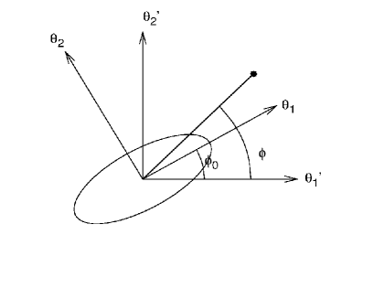
Figure 1: The coordinate systems and relative angles used. The star represents the location of one background galaxy.

In this section, we first use the analytic singular isothermal ellipsoid (SIE) model to illustrate the results before we study the more realistic elliptical Navarro-Frenk-White (eNFW) profile.

4.1 SIE model

We adopt an SIE model for the foreground lens. The SIE model includes 3 parameters: the Einstein radius $\theta_{\rm E}$, which defines the scale of the lens and is related to the mass or velocity dispersion (see Eq. 18); the halo ellipticity, defined by $\epsilon=(\theta_{a}-\theta_{b})/(\theta_{a}+\theta_{b})$ (or equivalently by the axial ratio $f=\theta_{b}/\theta_{a})$, where $\theta_{a},\theta_{b}$ are the major and minor axes; and the halo orientation $\phi_{0}$.

The lensing properties of the halo, such as shear and flexion, are calculated at the background galaxies positions $(\theta_{1}^{\prime},\theta_{2}^{\prime})$. The image reference frame relates to the halo reference frame through the rotation $\theta_{1}=\theta_{1}^{\prime}\cos\phi_{0}+\theta_{2}^{\prime}\sin\phi_{0}$, $\theta_{2}=-\theta_{1}^{\prime}\sin\phi_{0}+\theta_{2}^{\prime}\cos\phi_{0}\,$, where $\phi_{0}$ is the halo orientation (see Fig. 1 for an illustration).

The dimensionless surface mass density produced by an SIE halo at the location $(\theta_{1}^{\prime},\theta_{2}^{\prime})$ of a background galaxy is given by

$$\kappa(\theta_{1}^{\prime},\theta_{2}^{\prime}|\theta_{\rm E},\epsilon,\phi_{0})={\theta_{\rm E}\over\rho},$$ (13)

with $\rho(\theta_{1},\theta_{2})$ defined by

$$\rho=\sqrt{\theta_{1}^{2}f^{2}+\theta_{2}^{2}}.$$ (14)

The halo produces the following shear and flexion fields for a source at $z_{s}=\infty$:

$${\gamma(\theta_{1}^{\prime},\theta_{2}^{\prime})\over\theta_{\rm E}} = -{\theta_{1}^{2}-\theta_{2}^{2}\over\rho\theta^{2}}-{\rm i}\;{2\theta_{1}\theta_{2}\over\rho\theta^{2}};$$ (15)

$${{\cal F}(\theta_{1}^{\prime},\theta_{2}^{\prime})\over\theta_{\rm E}} = -{\theta_{1}f^{2}\over\rho^{3}}-{\rm i}\;{\theta_{2}\over\rho^{3}},$$ (16)

$${{\cal G}(\theta_{1}^{\prime},\theta_{2}^{\prime})\over\theta_{\rm E}} = -\left({2\theta_{1}^{3}-6\theta_{1}\theta_{2}^{2}\over\theta^{4}\rho}+{f^{2}\theta_{1}^{3}-f^{2}\theta_{1}\theta_{2}^{2}-2\theta_{1}\theta_{2}^{2}\over\theta^{2}\rho^{3}}\right)$$ (17)

$$-{\rm i}\left({6\theta_{1}^{2}\theta_{2}-2\theta_{2}^{3}\over\theta^{4}\rho}+{\theta_{1}^{2}\theta_{2}-\theta_{2}^{3}+2f^{2}\theta_{1}^{2}\theta_{2}\over\theta^{2}\rho^{3}}\right),$$

where $\theta=\sqrt{\theta^{2}_{1}+\theta_{2}^{2}}$ and $f$ is the axial ratio. The shear and flexion will be scaled to different redshifts for other values of $z_{s}$, according to Eq. (5).

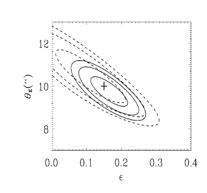
Figure 2: Marginalized SIE $68\%$, $95\%$ and $99\%$ credible regions using shear data only (dashed) and combined shear + flexion data (solid). Left panel: $(\theta_{\rm E}$-$\epsilon$) plane. Right panel: $(\phi_{0}$-$\epsilon)$ plane. The cross shows the fiducial input model.

4.2 Simulated fields

We place a halo, with fiducial parameter values $\theta_{\rm E}=10^{\prime\prime}$, $\epsilon=0.15$, $\phi_{0}=0$ and redshift $z_{\rm d}=0.6$, at the center of a $1.5^{\prime}\times 1.5^{\prime}$ field. The Einstein radius $\theta_{\rm E}$ for a singular isothermal spherical halo with velocity dispersion $\sigma_{v}$ is given by

$$\theta_{\rm E}=4\pi\left(\sigma_{v}\over c\right)^{2}{D_{\rm ds}\over D_{\rm s}}.$$ (18)

Thus for the case of $\theta_{\rm E}=10^{\prime\prime}$ and $z_{\rm s}=1.45$ (implying $D_{\rm ds}/D_{\rm s}=0.5$), the velocity dispersion is about $840$ km/s, corresponding to a large group or a cluster.

We then place 80 background galaxies in the field at random positions. A redshift is assigned to each galaxy according to a Gamma distribution with $z_{0}=1/3$,

$$p(z)={z^{2}\over 2z_{0}^{3}}{\rm exp}\left(-{z\over z_{0}}\right),$$ (19)

which peaks at $z=2/3$ and has a mean redshift of $\langle z\rangle=3z_{0}=1$. The source density corresponds to space-based observing conditions. It is compatible with the density of the weak lensing source galaxies observed in the COSMOS field (Schrabback et al. 2010).

The lensing shear and flexion components are computed for each galaxy according to the formula given in the previous section and using the cosmological weight function defined in Eq. (4).

We add noise to the shear and flexion signals. The shear noise is generated from a Gaussian distribution with $\sigma_{e}=0.2$ per shear component, and the flexion noise is generated from a Gaussian distribution with $\sigma_{\cal F}=0.03/^{\prime\prime}$ and $\sigma_{\cal G}=0.04/^{\prime\prime}$ per flexion component. Galaxies with shear absolute value larger than 0.9 are discarded from the analysis. This corresponds to about a few percent of the sample. We further discard, from the flexion analysis: 1) galaxies with flexion absolute value larger than $0.5/^{\prime\prime}$, since correct flexion estimates cannot be obtained in very strongly distorted images (see Schneider & Er 2008). 2) galaxies with small flexions ($|{\cal F}|<0.005/^{\prime\prime}$), which are exceedingly difficult to measure due to their low signal-to-noise ratios. 3) galaxies located at high redshift ($z>1.0$), which are too faint or too small to allow for a reliable flexion measurement (Okura et al. 2008). 4) galaxies located at low redshift ($z<0.61$) are also discarded since they are either below the lens redshift or too close to the lens to be efficiently lensed. In the end, we discard about $70\%$ of the flexion data in our analysis.

4.3 SIE results

We perform a likelihood analysis to assess how well the fiducial model can be recovered given the noisy shear and the two noisy flexion components in the simulated data.

The theoretical predictions are calculated using Eqs. (15)-(17) and the three parameters $\theta_{\rm E}$, $\epsilon$ and $\phi_{0}$ are varied. We use the following flat priors on the 3 free parameters. Firstly, the orientation $\phi_{0}$ could in principle be constrained independently by the shape of the luminous host object. However, there might be a systematic difference between the host orientation and the dark matter halo orientation. This misalignment appears to be small for elliptical galaxies (Keeton et al. 1998). We assume the polar angle of the orientation of the halo is distributed in a range smaller than $\pi/4$ with respect to the known orientation of the host. Secondly, we restrict the ellipticity to the range between 0.0 and 0.4. Ellipticity can be constrained using the morphologies of the lensing hosts. Finally, cluster studies using complementary approaches from kinematics and X-ray observations should allow us to independently constrain the halo mass, or $\theta_{\rm E}$. We allow about $30\%$ uncertainty around the input value and restrict $\theta_{\rm E}$ to the range $[7^{\prime\prime},13^{\prime\prime}]$ in our analysis.

Figure 2 shows the resulting credible contours for the SIE halo parameters. Both shear and flexion amplitudes increase with halo mass and also increase, on average over source locations, with halo ellipticity, as shown in Fig. 3. Accordingly, the likelihood analysis produces an anti-correlated contour, as shown in Fig. 2 (left panel). Flexion is more sensitive to a change in the halo ellipticity than shear, producing tighter constraints. For the SIE model the introduction of flexion data produces a gain of a factor of 2 on the marginalized errors of ellipticity and mass (see Tab.1).

Figure 3: Amplitude of shear (dashed) and flexion (solid) at a typical location ($\theta_{1}^{\prime},\theta_{2}^{\prime}$)=($10^{\prime\prime},30^{\prime\prime}$) as function of the SIE halo ellipticity, normalized by the amplitude in the singular isothermal spherical model.

There is also a large improvement on the uncertainty of the halo orientation when using flexion data, as seen in the right panel of Fig. 2. To check the robustness of the result against sample variance we made various realizations of the noise and location of the background galaxies, having obtained similar results. We also made tests using a higher number of background galaxies, obtaining correspondingly tighter constraints.

These results assume perfectly known redshifts for the source galaxies. We introduce now a redshift uncertainty of $2\%$ on average to simulate photo-z errors, which increase with redshift (Bolzonella et al. 2000; Hildebrandt et al. 2010). The marginalized contours for SIE parameters are shown in Fig. 4. The impact of the redshift uncertainty is significant, due to the strong degeneracy between $\theta_{\rm E}$ and redshift, increasing the $1\sigma$ error on the $\theta_{\rm E}$ estimate by roughly a factor of 2. Furthermore, the redshift uncertainty produces a selection bias in realizations with excess of low-redshift sources, introducing a bias in the $\theta_{\rm E}$ estimate. Due to the anti-correlation found between $\theta_{\rm E}$ and $\epsilon$ in the SIE model, such selection bias will also affect the ellipticity estimate. On the other hand, we found no significant effect on the orientation.

	SIE		eNFW
	Shear	Shear + Flexion	Shear	Shear + Flexion
$\epsilon$	$0.115\pm 0.061$	$0.164\pm 0.035$	$0.242\pm 0.101$	$0.174\pm 0.060$
$\theta_{\rm E}(^{\prime\prime})$	$10.38\pm 0.78$	$9.75\pm 0.46$
$\kappa_{s}$			$0.256\pm 0.030$	$0.242\pm 0.022$
$\delta M$	$15\%$	$9\%$	$32\%$	$26\%$

Table 1: $1\sigma$ errors estimated for the parameters of both models using shear and shear+flexion data. For comparison between SIE and eNFW the uncertainties on lens strength parameters were converted into mass uncertainties in the last row. The mass of SIE model stands for the mass within the Einstein radius ($\theta_{\rm E}$), and the mass of eNFW model stands for $M_{200}$.

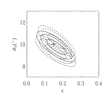
Figure 4: SIE $68\%$, $95\%$ and $99\%$ credible regions using shear and flexion data, marginalized over redshift uncertainty. The result of Fig. 2 is shown for comparison (solid contours). The cross shows the fiducial input model.

4.4 eNFW model

In order to test the universality of the result we perform our analysis on a more realistic model of halo density profile, adopting an eNFW model for the foreground lens halo. The NFW profile (Navarro et al. 1996, 1997) is widely used to model the halo of galaxy clusters. The dimensionless surface mass density of a spherical NFW halo is written as (Bartelmann 1996; Bacon et al. 2006)

$$\kappa(x)=2\kappa_{s}{f(x)\over x^{2}-1},$$ (20)

where $x$ is the dimensionless radius, the radius $r$ normalized by the scaling radius $r_{s}$ ($x\equiv r/r_{s}$), and the function $f(x)$ is given by

$$f(x)=\begin{cases}1-\dfrac{2}{\sqrt{x^{2}-1}}{\rm arctan}\sqrt{\dfrac{x-1}{x+1}}\;\;(x>1);\\ \\ 0\quad\quad\quad\quad\quad\quad\quad\quad\quad\quad\quad\;\;(x=1);\\ \\ 1-\dfrac{2}{\sqrt{1-x^{2}}}{\rm arctanh}\sqrt{\dfrac{1-x}{1+x}}\;\;(x<1).\\ \end{cases}$$ (21)

The physical properties of the halo are contained in the parameter $\kappa_{s}=\rho_{\rm crit}r_{s}\Delta_{c}/\Sigma_{\rm cr}$, where $\Delta_{c}$ is the dimensionless characteristic density. The halo mass is defined as $M_{200}=4/3\rho_{\rm crit}\pi r_{200}^{3}$, where $r_{200}=r_{s}\,c$ and $c$ is the concentration parameter (see the appendix in Navarro et al. 1997).

For an elliptical halo the dimensionless radius at a point $(\theta_{1},\theta_{2})$, defined along the axes of the halo, becomes

$$x=\frac{\rho}{1-\epsilon}\,\frac{D_{\rm d}}{r_{s}}.$$ (22)

The halo ellipticity is defined by $\epsilon=(\theta_{a}-\theta_{b})/(\theta_{a}+\theta_{b})$ (or equivalently by the axial ratio $f=\theta_{b}/\theta_{a}$), where $\theta_{a}$, $\theta_{b}$ are the major and minor axes.

The lensing properties of the eNFW halo can be calculated numerically given an arbitrary normalized halo convergence (Keeton 2001; Hawken & Bridle 2009) as follows.

The shear and flexion are second and third order derivatives of the lensing potential $\psi$:

$$\gamma = {1\over 2}(\psi_{11}-\psi_{22})+{\rm i}\psi_{12};$$ (23)

$${\cal F} = {1\over 2}\left[\psi_{111}+\psi_{122}+{\rm i}(\psi_{112}+\psi_{222})\right];$$ (24)

$${\cal G} = {1\over 2}\left[\psi_{111}-3\psi_{122}+{\rm i}(3\psi_{112}-\psi_{222})\right],$$ (25)

where subscripts denote partial differentiation. The second and third order derivatives of the lensing potential, for an eNFW dark matter halo at a position $(x,y)$ on the image plane, are given by

$$\psi_{11} = 2fx^{2}K_{0}+fJ_{0};$$ (26)

$$\psi_{22} = 2fy^{2}K_{0}+fJ_{1};$$ (27)

$$\psi_{12} = 2fxyK_{1};$$ (28)

$$\psi_{111} = 6fxK_{0}+4fx^{3}L_{0};$$ (29)

$$\psi_{222} = 6fyK_{2}+4fy^{3}L_{3};$$ (30)

$$\psi_{112} = 2fyK_{1}+4fx^{2}yL_{1};$$ (31)

$$\psi_{122} = 2fxK_{1}+4fy^{2}xL_{2}.$$ (32)

Here

$$J_{n}(x,y) = \int_{0}^{1}\frac{\kappa(\xi(u)^{2}){\rm d}u}{\left[1-(1-f^{2})u\right]^{n+1/2}},$$ (33)

$$K_{n}(x,y) = \int_{0}^{1}\frac{u\,\kappa^{\prime}\,(\xi(u)^{2})\,du}{[1-(1-f^{2})u]^{n+1/2}},$$ (34)

$$L_{n}(x,y) = \int_{0}^{1}\frac{u^{2}\,\kappa^{\prime\prime}\,(\xi(u)^{2})du}{[1-(1-f^{2})u]^{n+1/2}},$$ (35)

are one-dimensional integrals, where $f$ is the axis ratio of the lens and $\kappa^{\prime}$ and $\kappa^{\prime\prime}$ are the first and second order derivatives of the convergence, e.g. $\kappa^{\prime}(\xi^{2})={\rm d}\kappa(\xi^{2})/{\rm d}(\xi^{2})$. The convergence $\kappa$ is written as a function of the ellipse coordinate $\xi(u)$ given by

$$\xi(u)^{2}=u\left(x^{2}+{y^{2}\over 1-(1-f^{2})u}\right).$$ (36)

Notice here we need to use $x^{2}$ instead of $x$ as the independent variable in $\kappa(x)$.

Figure 5: Marginalized eNFW $68\%$, $95\%$ and $99\%$ credible regions using shear data only (dashed) and combined shear + flexion data (solid). Left panel: $(\theta_{\rm E}$-$\epsilon$) plane. Right panel: $(\phi_{0}$-$\epsilon)$ plane. The cross shows the fiducial input model.

4.5 eNFW results

In the eNFW model, we consider 3 free parameters: $(\kappa_{s},\epsilon,\phi)$. For our fiducial halo we use a halo mass of $M_{200}=1.8\times 10^{14}M_{\odot}$, a concentration parameter of $c=7.2$, and place the halo at redshift $z_{\rm d}=0.6$. This implies $\kappa_{s}=0.227$. For the ellipticity we choose $\epsilon=0.15$ and for position angle $\phi_{0}=0$.

The theoretical predictions are calculated numerically and the three parameters $\kappa_{s}$, $\epsilon$ and $\phi_{0}$ are varied. Similar to the SIE analysis, we place 80 background galaxies at random positions in the same field, and randomize their shear and flexion values. The same filter to the data is employed to discard the unmeasurable data in the analysis. We perform a likelihood analysis restricting $\phi_{0}$ to the range $[-\pi/4,\pi/4]$, using the range $[0.15,0.3]$ for $\kappa_{s}$ and $[0,0.4]$ for the ellipticity $\epsilon$.

Figure 5 shows the resulting credible intervals for the eNFW halo parameters. Overall, the constraints are looser than in the SIE model, which has a higher signal-to-noise ratio. The effective number of flexed background images available for the analysis after discarding is lower than that in the SIE analysis by about $15\%$.

The constraints from shear information alone, using priors similar to the ones used in the SIE analysis, are dominated by the priors. Hence, shear data do not add much information to observations of the luminous host and complementary probes of mass (e.g. X-ray).

Figure 6: Amplitude of shear (dashed) and flexion (solid) at a typical location $(\theta_{1}^{\prime},\theta_{2}^{\prime})=(10^{\prime\prime},30^{\prime\prime})$ as a function of the eNFW halo ellipticity, normalized by the amplitude in the spherical NFW model.

Ellipticity and lens strength are now positively correlated in the shear signal due to the decreasing shear amplitude with ellipticity, as shown in Fig. 6. The addition of flexion data decreases the correlation. Once again, flexion is more sensitive to the change in the halo ellipticity than shear. Indeed, the tangential shear mainly depends on the lens strength ($\theta_{\rm E}$ or $\kappa_{s}$) and depends weakly on the halo ellipticity, while the cross shear component is independent of ellipticity. On the other hand, both flexion components depend on the halo ellipticity and orientation $\phi_{0}$. This allows for a tighter constraint when including flexion information. In Table 1 the shear and flexion marginalized constraints on the ellipticity and strength parameters are roughly a factor of 1.5 tighter than the corresponding shear constraints. Notice that the effective gain of using flexion is larger than this factor. Here the shear constraint, contrary to the combined one, is dominated by the prior; with a wider prior range the shear constraint would be looser.

We also stress that the eNFW model constraints are not marginalized on all halo parameters, since the scaling radius $r_{s}$ is kept fixed in the analysis. Finally, we checked the results against sample variance making various realizations of noise and location of the background galaxies, similar results are found.

5 Conclusions

In this paper, we study the potential of weak lensing flexion in the study of galaxy cluster haloes. We use mock data including shear, $\cal F$ flexion, $\cal G$ flexion and redshift information. We find that the inclusion of flexion significantly improves the estimate of foreground haloes parameters, although the details are model-dependent. In particular, in the case of a SIE halo, the presence of a mass-ellipticity anti-correlation implies that analyses where the halo is incorrectly assumed to be spherical will overestimate the halo mass. On the other hand, we did not find significant correlation between the halo mass and ellipticity in the eNFW model.

The noise in the mock data is determined by the dispersion of the intrinsic shear and flexion distributions, and by the density of background galaxies. After applying stringent cuts in the data, we are left with a galaxy density of roughly 10 arcmin^-2. Our approach assumes that the flexion estimators are linear in the flexion observables and the point spread function can be removed without producing a bias. In reality, the noise of flexion estimators can be complicated and non-Gaussian. An accurate study of flexion noise is important to evaluate the estimated error.

The analysis considers a single cluster halo. This approach is not possible if the number density of background galaxies is low. In that case, stacking of several halo fields can be used to increase the number of background images and thus the signal-to-noise. That approach requires the alignment of the major axis of various foreground galaxies and selecting haloes with similar properties, for example similar shapes of their central galaxies. Such stacking analysis can constrain the halo shapes more tightly, and as a function of other halo properties, e.g. mass.

Our results emphasize that a combined weak lensing analysis will be a useful technique for precise measurements of the properties of galaxy or cluster haloes from future weak lensing surveys, such as EUCLID.

References

- Allgood et al. (2006) Allgood B., Flores R. A., Primack J. R., Kravtsov A. V., Wechsler R. H., Faltenbacher A., Bullock J. S., 2006, MNRAS, 367, 1781
- Bacon et al. (2010) Bacon D. J., Amara A., Read J. I., 2010, MNRAS, 409, 389
- Bacon et al. (2006) Bacon D. J., Goldberg D. M., Rowe B. T. P., Taylor A. N., 2006, MNRAS, 365, 414
- Bailin & Steinmetz (2005) Bailin J., Steinmetz M., 2005, ApJ, 627, 647
- Bartelmann (1996) Bartelmann M., 1996, A&A, 313, 697
- Bolzonella et al. (2000) Bolzonella M., Miralles J., Pelló R., 2000, A&A, 363, 476
- Brainerd et al. (1996) Brainerd T. G., Blandford R. D., Smail I., 1996, ApJ, 466, 623
- Bullock (2002) Bullock J. S., 2002, in P. Natarajan ed., The Shapes of Galaxies and their Dark Halos Shapes of Dark Matter Halos. pp 109–113
- Cain et al. (2011) Cain B., Schechter P. L., Bautz M. W., 2011, ApJ, 736, 43
- De Filippis et al. (2005) De Filippis E., Sereno M., Bautz M. W., Longo G., 2005, ApJ, 625, 108
- Er et al. (2010) Er X., Li G., Schneider P., 2010, arXiv:1008.3088
- Er et al. (2011) Er X., Mao S., Xu D.D, Cao Y., 2011, MNRAS, 417, 2197
- Er & Schneider (2011) Er X., Schneider P., 2011, A&A, 528, A52
- Fluke & Lasky (2011) Fluke C. J., Lasky P. D., 2011, MNRAS, 416, 1616
- Goldberg & Bacon (2005) Goldberg D. M., Bacon D. J., 2005, ApJ, 619, 741
- Goldberg & Leonard (2007) Goldberg D. M., Leonard A., 2007, ApJ, 660, 1003
- Goldberg & Natarajan (2002) Goldberg D. M., Natarajan P., 2002, ApJ, 564, 65
- Hawken & Bridle (2009) Hawken A. J., Bridle S. L., 2009, MNRAS, 400, 1132
- Hilbert et al. (2011) Hilbert S., Gair J. R., King L. J., 2011, MNRAS, 412, 1023
- Hildebrandt et al. (2010) Hildebrandt H., Arnouts S., Capak P., Moustakas L. A., Wolf C., Abdalla F. B., Assef R. J., Banerji M., Benítez N., Brammer G. B., Budavári T., Carliles S., Coe D., Dahlen T., Feldmann R., Gerdes D., Gillis B., Ilbert O., Kotulla R., Lahav O., Li I. H., Miralles J., Purger N., Schmidt S., Singal J., 2010, A&A, 523, A31
- Hoekstra et al. (2004) Hoekstra H., Yee H. K. C., Gladders M. D., 2004, ApJ, 606, 67
- Hudson et al. (1998) Hudson M. J., Gwyn S. D. J., Dahle H., Kaiser N., 1998, ApJ, 503, 531
- Irwin & Shmakova (2006) Irwin J., Shmakova M., 2006, ApJ, 645, 17
- Jing & Suto (2002) Jing Y. P., Suto Y., 2002, ApJ, 574, 538
- Kauffmann et al. (1993) Kauffmann G., White S. D. M., Guiderdoni B., 1993, MNRAS, 264, 201
- Kazantzidis et al. (2004) Kazantzidis S., Kravtsov A. V., Zentner A. R., Allgood B., Nagai D., Moore B., 2004, ApJ, 611, L73
- Keeton (2001) Keeton C. R., 2001, ArXiv:astro-ph/0102341
- Keeton et al. (1998) Keeton C. R., Kochanek C. S., Falco E. E., 1998, ApJ, 509, 561
- Lee & Suto (2004) Lee J., Suto Y., 2004, ApJ, 601, 599
- Leonard et al. (2007) Leonard A., Goldberg D. M., Haaga J. L., Massey R., 2007, ApJ, 666, 51
- Leonard et al. (2009) Leonard A., King L. J., Wilkins S. M., 2009, MNRAS, 395, 1438
- Mandelbaum et al. (2006) Mandelbaum R., Seljak U., Kauffmann G., Hirata C. M., Brinkmann J., 2006, MNRAS, 368, 715
- Mellier (1999) Mellier Y., 1999, ARA&A, 37, 127
- Munshi et al. (2008) Munshi D., Valageas P., van Waerbeke L., Heavens A., 2008, Phys. Rep., 462, 67
- Navarro et al. (1996) Navarro J. F., Frenk C. S., White S. D. M., 1996, ApJ, 462, 563
- Navarro et al. (1997) Navarro J. F., Frenk C. S., White S. D. M., 1997, ApJ, 490, 493
- Okura et al. (2007) Okura Y., Umetsu K., Futamase T., 2007, ApJ, 660, 995
- Okura et al. (2008) Okura Y., Umetsu K., Futamase T., 2008, ApJ, 680, 1
- Reblinsky (2000) Reblinsky K., 2000, A&A, 364, 377
- Schneider (2006) Schneider P., 2006, Weak Gravitational Lensing. p. 269
- Schneider & Er (2008) Schneider P., Er X., 2008, A&A, 485, 363
- Schneider & Rix (1997) Schneider P., Rix H.-W., 1997, ApJ, 474, 25
- Schrabback et al. (2010) Schrabback T., Hartlap J., Joachimi B., Kilbinger M., Simon P., Benabed K., Bradač M., Eifler T., Erben T., Fassnacht C. D., High F. W., Hilbert S., Hildebrandt H., Hoekstra H., Kuijken K., Marshall P. J., Mellier Y., Morganson E., Schneider P., Semboloni E., van Waerbeke L., Velander M., 2010, A&A, 516, A63
- Sereno et al. (2006) Sereno M., De Filippis E., Longo G., Bautz M. W., 2006, ApJ, 645, 170
- Shapiro et al. (2010) Shapiro C., Bacon D. J., Hendry M., Hoyle B., 2010, MNRAS, 404, 858
- Sheldon et al. (2004) Sheldon E. S., Johnston D. E., Frieman J. A., Scranton R., McKay T. A., Connolly A. J., Budavári T., Zehavi I., Bahcall N. A., Brinkmann J., Fukugita M., 2004, AJ, 127, 2544
- Springel et al. (2004) Springel V., White S. D. M., Hernquist L., 2004, in S. Ryder, D. Pisano, M. Walker, & K. Freeman ed., Dark Matter in Galaxies Vol. 220 of IAU Symposium, The shapes of simulated dark matter halos. p. 421
- Springel et al. (2005) Springel V., White S. D. M., Jenkins A., Frenk C. S., Yoshida N., Gao L., Navarro J., Thacker R., Croton D., Helly J., Peacock J. A., Cole S., Thomas P., Couchman H., Evrard A., Colberg J., Pearce F., 2005, Nature, 435, 629
- Tyson et al. (1984) Tyson J. A., Valdes F., Jarvis J. F., Mills Jr. A. P., 1984, ApJ, 281, L59
- Velander et al. (2011) Velander M., Kuijken K., Schrabback T., 2011, MNRAS, 412, 2665
- Viola et al. (2011) Viola M., Melchior P., Bartelmann M., 2011, ArXiv 1107.3920
- Wang & White (2007) Wang J., White S. D. M., 2007, MNRAS, 380, 93
- Wang et al. (2010) Wang Y., Park C., Hwang H. S., Chen X., 2010, ApJ, 718, 762