AN AUTOMATIC METHOD FOR EXTREME-ULTRAVIOLET DIMMINGS ASSOCIATED WITH SMALL-SCALE ERUPTION

Abstract

Small-scale extreme ultraviolet (EUV) dimming often surrounds sites of energy release in the quiet Sun. This paper describes a method for the automatic detection of these small-scale EUV dimmings using a feature based classifier. The method is demonstrated using sequences of 171Å images taken by STEREO/EUVI on 13 June 2007 and by SDO/AIA on 27 August 2010. The feature identification relies on recognizing structure in sequences of space-time 171Å images using the Zernike moments of the images. The Zernike moments space-time slices with events and non-events are distinctive enough to be separated using a Support Vector Machine (SVM) classifier. The SVM is trained using 150 event and 700 non-event space-time slices. We find a total of 1217 events in the EUVI images and 2064 events in the AIA images on the days studied. Most of the events are found between latitudes -35^∘ and +35^∘. The sizes and expansion speeds of central dimming regions are extracted using a region grow algorithm. The histograms of the sizes in both EUVI and AIA follow a steep power law with slope about -5. The AIA slope extends to smaller sizes before turning over. The mean velocity of 1325 dimming regions seen by AIA is found to be about 14 km s^-1.

1 Introduction

Extreme ultraviolet (EUV) dimming surrounding small bursts of EUV brightening in the quiet Sun were first noticed by Innes et al. (2009) in 171Å images taken by the Extreme UltraViolet Imager (EUVI) on STEREO. The dimmings are usually more extended and last longer than the brightening (Podladchikova et al. 2010; Innes et al 2010). They seem to be related chromospheric eruptions at the junctions of supergranular cells (Innes et al. 2009). In 171Å solar disk images small-scale eruptions have similar characteristics to face-on CMEs but on a smaller scale. Apart from microflare brightening and dimming of the surrounding corona, several events have wave-like features propagating from the eruption site.

Podladchikova et al. (2010) focused on the small-scale diffuse coronal fronts and their associated dimmings for a couple of events. The coronal wave and dimming properties were extracted using a semi-automatic algorithm adapted from their method developed for CMEs (Podladchikova & Berghmans 2005). They show that waves develop from micro-flaring sites and propagate up to a distance of 40,000 km in 20 min. The dimming region is two orders of magnitude smaller than for large-scale events. The waves associated with the micro-eruptions had a velocity of 17 km s^-1, and were diagnosed as slow mode, propagating almost perpendicular to the background magnetic field.

Innes et al. (2009) estimated a rate of 1400 events per day over the whole Sun by picking out events by eye in a period of 24 hours. Now the Solar Dynamics Observatory/Atmospheric Imaging Assembly (SDO/AIA) is providing full Sun images through ten UV and EUV filters with a cadence of about one image every second. To optimize statistical analyses of various kinds of solar phenomena, it is necessary to develop automatic detection techniques. Aschwanden (2010) gives an extensive overview of solar image processing techniques that are used in automated feature detection algorithms. One of the modules in the Computer Vision Center for SDO is designed to automatically detect and extract coronal dimmings from AIA images (Attrill & Wills-Davey 2010).

Here, we give an automatic method to detect small-scale dimmings in the 171Å STEREO/EUVI and SDO/AIA images using Zernike moments and the Support Vector Machine (SVM) classifier. The method exploits the characteristics of the Zernike moments in order to represent event/non-event patterns. The Zernike moments are invariant to rotation, scaling, and translation, and this allows the proposed method to detect events even if they are translated, scaled or rotated. First the Zernike moments are extracted for a selection of events and non-events, and fed into the SVM as training data sets so that it can successfully identify events/non-events in subsequent 171Å image sequences.

The paper layout is as follows: data reduction is discussed in Section 2; Zernike moments are explained in Section 3; the Support Vector Machine is discussed in Section 4; and the results and conclusions are presented in Section 5.

2 Data Reduction

EUVI on the STEREO spacecraft takes images of the Sun through four different EUV filters (171Å, 195Å, 284Å  and 304Å) (Howard et al. 2008). In the present work we have restricted ourselves to 171Å images with a time cadence of 2.5 min and a pixel size 1.6″, taken on 13 June 2007. First the recorded images were calibrated using the SolarSoft routine secchi$\_$prep.pro.

SDO is designed to study the solar atmosphere on small scales of space and time and in many wavelengths simultaneously (http://sdo.gsfc.nasa.gov/mission/instruments.php). For this study we have used AIA level 1.5 171Å data from the series aia_test.synoptic2 recorded on 27 August 2010. These are binned data (1024$\times$1024) with a pixel size 2.4″ and an image interval of 90 s. To keep the image and pixel sizes approximately the same in both datasets the SDO images were rebinned to 2048$\times$2048 pixels.

Innes et al. (2009) show that events that have expanding dimming regions produce distinctive diagonal structures in space-time EUV images (Figures 1 and 2). Our automatic procedure therefore systematically scans through space-time blocks of the data. A flowchart of the algorithm is shown in Figure 3. First all $N_{t}$ 171Å images of size $N_{x}\times N_{y}$ from each data set were calibrated and de-rotated to the start time of the data series. Then following Innes et al. (2009) space-time slices through the data were made by averaging 3 consecutive pixels along the Sun-y direction to give a Sun-x versus time image for every third Sun-y position of size $N_{x}\times N_{t}$. Then for each space-time image, a small region, starting from $x1=1,t1=1$ with the size $\Delta x=S_{1}$ and $\Delta t=S_{1}$ is extracted. The location, $x_{min}$, and time, $t_{min}$, of the minimum intensity inside this small region is determined. This gives the location of the deepest dimming in the region. In step 3, a larger region is selected around the minimum intensity position ($x_{min}$, $t_{min}$) with size $\Delta x=S_{2}$ and $\Delta t=S_{2}$. The Zernike moments, $Z_{pq}$, of this section of the image are computed. The magnitudes of the moments are fed to the SVM classifier. The code picks up a label 1 for an event class and 2 for a non-event class. If it is an event, the location $x_{min}$ and time $t_{min}$ are saved. Then the small box is moved first in space until the end of the grid is reached and then in time. By repeating this for each of the $N_{y}/3$ slices, all parts of the data are investigated.

Neighbouring $y$-slices pick-up different parts of the same event. Events found in neighbouring space-time slices are grouped together so that the expansion speed and dimming size can be measured in both the $x$ and $y$ directions.

3 Zernike moments

In the past decades, various moment functions (Legendre, Zernike, etc) due to their abilities to represent the image features have been proposed for describing images (Hu 1962). The Zernike polynomials form a complete set of orthogonal polynomials. The orthogonal property enables the contribution of each moment to be unique and independent of the information in an image. Therefore the Zernike moments, $Z_{pq}$, for each feature are unique. Space-time images of a slice on the Sun would look like simple vertical stripes if there is no activity. If there is a brightening or dimming with no flows the stripes change intensity but keep their basic vertical structure. When an eruption occurs and the region expands, diagonal structures appear crossing the background vertical stripes. This change in structure is reflected in the pattern of the Zernike moments, and the high Zernike coefficients, $Z_{pq}$, appear in blocks. If we select a small box on the dimming region and then compute the moments the block structure in $Z_{pq}$ is not as clear as for a slightly large region that takes in the surroundings as well as the dimming region because it is the structure change that is registered in the moments.

Using a Matlab code, we calculated the Zernike moments of order up to $p=31$. The repetition number, $q$, satisfied $p-|q|$ is even. This gives a $(q,p)$ set labelled from 1 to 528. The Zernike moments of three events and three non-events are shown in Figures 4 and 5, respectively. As shown in the figures, the real part of the Zernike moments are clearly different for event and non-events features. The events have a well-defined block structure. For non-events features, we see some block structure but it is different from the event type of block. These differences gives us confidence in applying a Support Vector Machine (SVM) classifier to identify events in space-time slices.

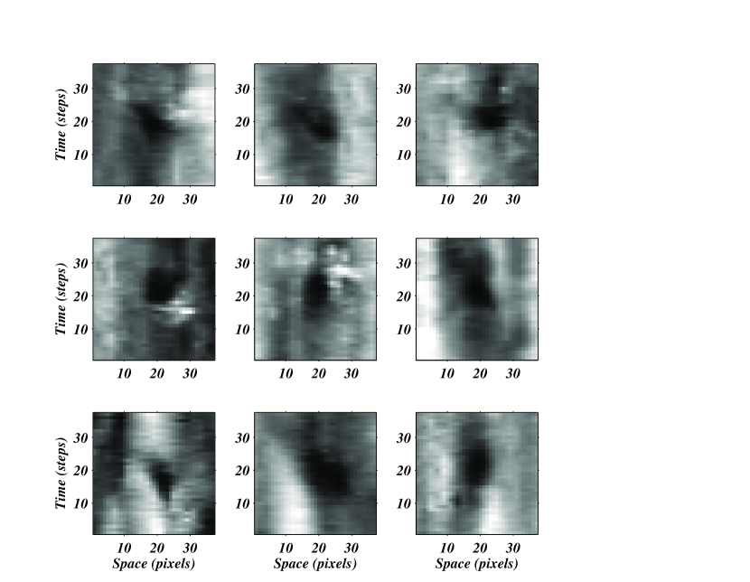
Figure 1: Examples of events shown as space-time slices (SDO/AIA). The frames are 37 pixels$\times$37 time steps. Each pixel is 1.2″ across and each time step is 90 s.

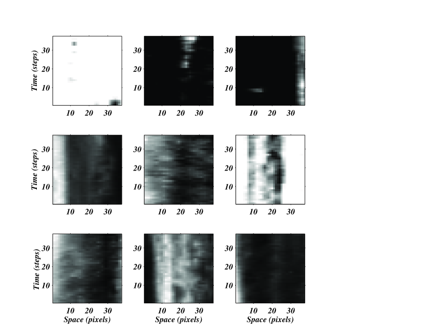
Figure 2: Examples of non-events shown as space-time slices (SDO/AIA). The frames are 37 pixels$\times$37 time steps. Each pixel is 1.2″ across and each time step is 90 s.

4 Support Vector Machine

The support vector machine (SVM) is a generation learning system based on statistical learning theory. It was successfully applied to text categorization, image classification, etc. SVM is basically defined for two class problems. It finds the optimal hyperplane which maximizes the distance between the nearest examples of both classes. It is a supervised learning method based on kernel functions (Burges 1998). We use the least square SVMlab Toolbox classifier in the Matlab environment with the Gaussian Radial Basis Function as the SVM kernal (Gunn 1997).

To prepare (train) the network we computed the Zernike moments of 150 events and 700 non-events. Once the SVM had been trained it could be used to classify the space-time images and find events.

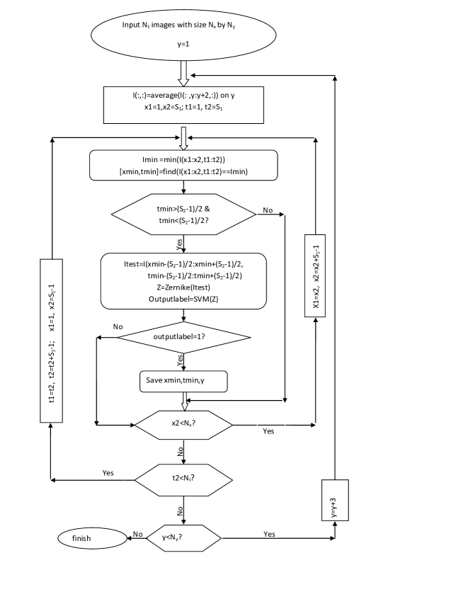
Figure 3: A flowchart representation for the automatic detection scheme for small dimmings. The parameters used for EUVI were $S_{1}=13$ and $S_{2}=31$, and for AIA $S_{1}=15$ and $S_{2}=37$.

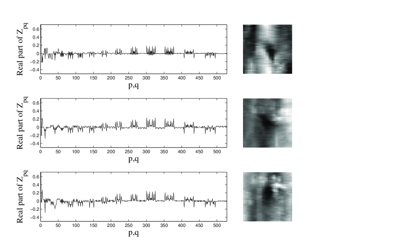
Figure 4: Real part of Zernike moment, $Z_{pq}$, of three events.

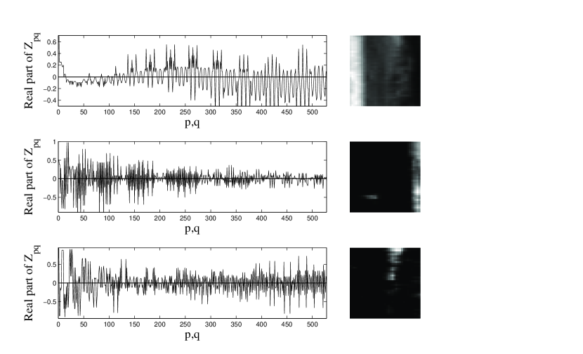
Figure 5: Real part of Zernike moment of the three non-events.

5 Results and Conclusions

5.1 Results

The automatic detection scheme for small-scale EUV dimmings has been applied to full Sun STEREO/EUVI and SDO/AIA 171Å data. On 13 June 2007, 1217 events were detected from the EUVI images. This is approximately twice the rate found by Innes et al. (2009) by eye for the same dataset. In the AIA images, 2064 events were detected on 27 August 2010. AIA is therefore giving another factor two in event rate. Figure 6 shows the positions of events found during 20 min of EUVI and AIA images.

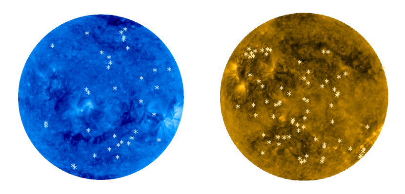
Figure 6: Positions of events detected in 20 min by EUVI (left) and AIA.

The event numbers from EUVI are plotted versus time, Sun-x, and Sun-y in Figure 7. We see that approximately 60 events were detected every hour. On average, there are 45 events per 50″ in both Sun-x and Sun-y. The numbers for AIA were double the EUVI numbers: 115 events per hour and 100 events for every 50″ in space. For both EUVI and AIA, the events are mostly found in the central part of the disk (between +35 degrees and -35 degrees). They are most easily identified against the quiet Sun because in active regions they disappear into the general background activity and off-limb there is too much line-of-sight confusion (Innes et al. 2009).

To make an estimate of how reliable the algorithm is we checked 400 of the detected events. We found that 30 of them are not clear events, like those shown in Figure 8. We also checked for events that the algorithm missed and could not find any additional events. Therefore we may be over-estimating small events numbers by about 10%.

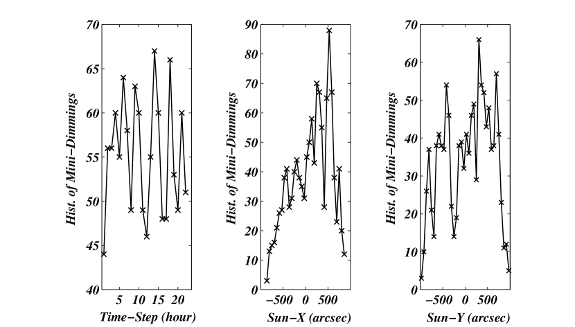
Figure 7: Number of events per hour and per 50″ detected in STEREO/EUVI images on 13 June 2007 plotted versus time (left) Sun-x (middle), and Sun-y (right).

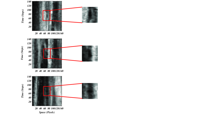
Figure 8: Three less clear events detected by SVM from AIA data.

The size and expansion rates of the dimmings have been computed with a region grow algorithm applied to the dimming region in the space-time slices (Figure 9). First a region (2 by 2) including the the original $x_{min}$ and $t_{min}$ is selected (left panel of Figure 9). Then the region is expanded to include all connected pixels which fall below the specified threshold. The width, $\Delta x$, is the maximum width of the dimming region. The event duration time interval, $\Delta t$, is the maximum along the time direction. Because the same event is often seen in several neighbouring $y$-slices, we first group events together and then apply the region grow algorithm to all events in the $x$ and $y$ directions. The longest time intervals and biggest widths are taken as the event sizes.

The size of the region depends on the threshold used. If it is too low then external dark areas will be included and if it is too high the region is too small. Our automatic method uses the full width at half maximum of the histograms of intensities of each space-time slice as the threshold. We tested this automatic level against manually chosen ones for a random 10% of the slices. Here we took special care to ensure no external areas were included. The difference between the width and duration of the two cases (automatic thresholds and manual thresholds) are calculated. Only two out of 140 events differed by more than 2 spatial pixels (1000 km). The duration has a slightly large uncertainty: 15 of the 140 events differed by for than 2 time steps (180 s).

The histograms of the AIA and EUVI sizes are shown in Figure 10. For larger events the slopes are the same (about -5) for both instruments. The difference between the two curves is that AIA curve turns over at a smaller size. The size refers to the central core dimmings not the event size so comparison with the large-scale CME distribution (Schrijver 2010) is not possible.

We compute the average velocity ($\Delta x/\Delta t$) for 1325 AIA dimming regions. The histogram of average velocities are shown in Figure 11. This histogram is similar to the distribution of CME’s speeds obtained from solar cycle 23 (Mittal & Narian 2009). The average velocities concentrate in the range of 3-80 km s^-1 with mean of 14 km s^-1. This is same as the average mini-filament velocity measured by Wang et al. (2000). Based on the uncertainly in space and duration the velocity uncertainties are small, typically 1 km s^-1. Only 5% have an uncertainly greater than 5 km s^-1.

5.2 Conclusion

An automatic method for the detection of small-scale EUV dimmings has been developed and tested on SDO/AIA and STEREO/EUVI 171Å images. The method exploits the fact that the Zernike moments of events that move have a specific pattern in space-time slices . This structure can be recognized by a Support Vector Machine classifier (SVM). Due to the invariant characteristics of the Zernike moments, the proposed method can detect events even if they are small or very faint.

At the moment we detect motion of the dimming front but the algorithm is not able to distinguish between events due to coronal field evolution with and without eruption. Since eruptive events almost always have sudden brightening at onset, we are working on an algorithm that uses event groups to find the position and intensity of the brightest pixel at the earliest time in a group. Then the event characteristics relative to this brightening can be used to classify events as eruptive or not.

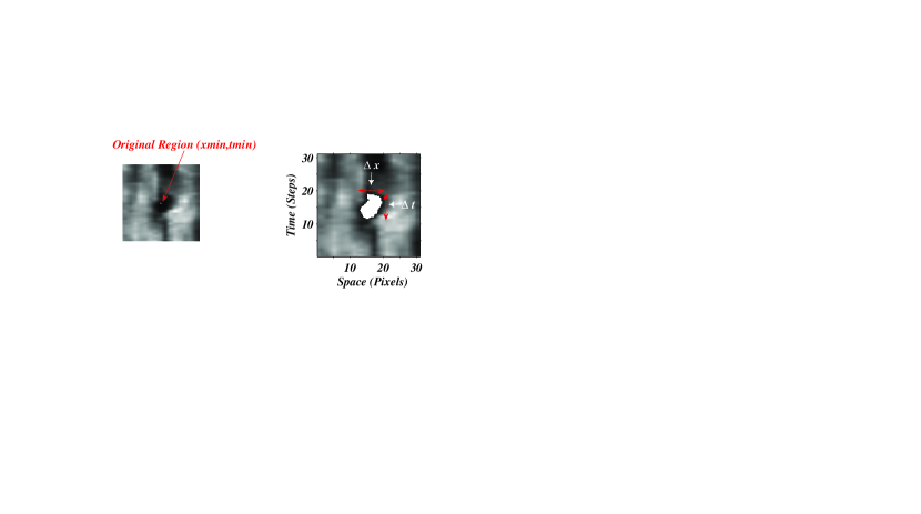
Figure 9: Demonstration of the mini-dimming extraction from a space-time slice, The frames are 7.8 arcsec by 10.9 min from SDO/AIA.

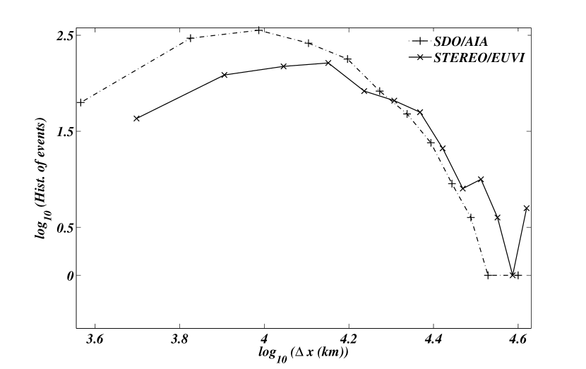
Figure 10: Histogram of small dimming events detected by AIA and EUVI.

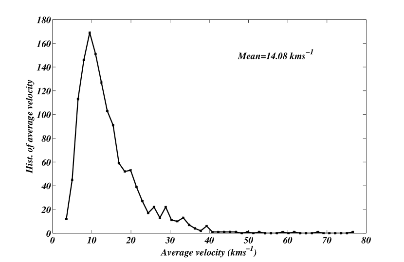
Figure 11: The histogram of average velocities of 1325 events are plotted versus velocities.

References

- (1) Attrill, G. D. R. & Wills-Davey, M. J., 2010, Sol. Phys., 262, 461.
- (2) Aschwanden, M. J., 2010, Sol. Phys., 262, 235.
- (3) Innes, D. E., Genetelli, A., Attie, R., & Potts, H.E. 2009, A&A, 495, 319.
- (4) Innes, D. E., McIntosh, S. W., and Pietarila, A. 2010, A&A, 517, L71.
- (5) Burges, C. J. C. 1998, Data Mining and Knowledge Discovery, 2, 121
- (6) Gunn, S. R., 1997, Technical Report, Image Speech and Intelligent Systems Research Group, University of Southampton.
- (7) Howard, R. A., Moses, J. D., Vourlidas, A., et al. 2008, Space Sci. Rev., 136, 67.
- (8) Hu, M. K. 1962, IRE Trans. on Information Theory, IT-8, 179.
- (9) Mittal, N. & Narain, U. 2009, New Astronomy, 14, 341.
- (10) Podladchikova, O.V., Berghmans, D. 2005, Sol. Phys., 228, 265.
- (11) Podladchikova, O., Vourlidas, A., Van der Linden, R. A. M., Wülser, J.-P.W, & Patsourakos, S. 2010, ApJ, 709, 369.
- (12) Schrijver, Carolus, J. 2010, ApJ, 710, 1480.
- (13) Wang, J., Li, W., Denker, C., et al. 2000, ApJ, 530, 1071.