A stochastic model for virus growth in a cell population

Abstract.

This work introduces a stochastic model for the spread of a virus in a cell population where the virus has two ways of spreading: either by allowing its host cell to live on and duplicate, or else by multiplying in large numbers within the host cell, causing the host cell to burst thereby letting the viruses enter new uninfected cells. The model is a kind of interacting Markov branching process. We focus in particular the probability that the virus population survives and how this depends on a certain parameter $\lambda$ which quantifies the ‘aggressiveness’ of the virus.

Our main goal is to determine the optimal balance between aggressive growth and long-term success. Our analysis shows that the optimal strategy of the virus (in terms of survival) is obtained when the virus has no effect on the host cell’s life-cycle, corresponding to $\lambda=0$. This is in agreement with experimental data about real viruses.

Keywords: Branching Processes, Interacting Branching Processes, Model for Virus Growth

Subject Classification Primary: 60J80, 60J85 Secondary: 60J27, 60J28, 92D15

1. Introduction

A virus is a simple parasitic organism consisting of compacted genetic material in a protein or lipid vessel. Viruses prey on living cells, such as bacterial or human cells, by penetrating the membrane of the cell and transferring their genetic material into the host. In order to multiply, the virus has two basic possibilities. The first option is for the virus to temporarily incorporate its genetic material in the host genome, and thereby be passively replicated along with the latter. The other option is to seize the host’s replication machinery and aggressively replicate, thereafter releasing its progeny in the surrounding medium. The ‘free virions’ must then attach to new host cells within a short time in order to survive. For many viruses, this process necessarily involves bursting the host cell, thereby killing it.

The technical term for the event that a virus bursts its host cell is lysis, and one says that the virus lyses the host cell. A virus which is incorporated into, and passivlely replicated along with, the host genome is said to be in the lysogenic state, or to employ the lysogenic strategy. Sometimes one speaks loosely of ‘the lytic strategy’ to denote that a virus ‘becomes lytic’, that is to say actively lyses the host cell. A lysogenic virus will eventuelly become lytic; in fact, it is well-established experimentally [13] that viruses in the lysogenic state will revert to the lytic strategy if the host cell is under stress and in danger of dying, enabling the virus to find a ‘safer’ host.

We introduce a stochastic model to investigate this behaviour. The model is a two-dimensional Markov process $(X(t),Y(t))_{t\geq 0}$, where $X(t)$ is the number of ‘healthy cells’ at time $t$, and $Y(t)$ is the number of ‘infected cells’ (i.e. cells having virus in them). Both components $(X(t))_{t\geq 0}$ and $(Y(t))_{t\geq 0}$ behave in many ways like branching processes, although there are dependencies between them. A healthy cell is replaced by a random number of new healthy cells at rate 1. This random number is independent of other events and drawn from a distribution $(p_{k})_{k\geq 0}$. Infected cells behave similarly, although they are replaced by $k$ new cells at rate $p_{k}$ if $k\geq 1,$ while they are replaced by 0 new cells (die) at the higher rate $p_{0}+\lambda$. Here $\lambda\geq 0$ is a parameter that reflects the negative impact of the virus on the hosts lifelength. When an infected cell dies (i.e.​ is replaced by 0 new cells), it bursts (lyses) and releases ‘free virions’. These free virions immediately enter a random number of healthy cells, thus converting them into infected cells. The number of new infections is independent of all other events, and is drawn from a distribution $(\gamma_{k})_{k\geq 0}$. The model is defined in detail in Section 2.1.

We are concerned with a fundamental question about the virus’ reproductive strategy, namely: what is the optimal level of ‘aggressiveness’ (balance of lysis to lysogeny) from the point of view of the virus? Here we interpret ‘optimality’ as maximizing the chance of the virus establishing itself in the cell population and, ultimatly, surviving in the long-term. We therefore study the extinction probability $\eta$ of the infected process $(Y(t))_{t\geq 0}$ (see Definition 2.1). We are interested in $\eta$, or rather $1-\eta$, as an indicator of the ‘fitness’ of the virus, and are mainly concerned with how it depends on $\lambda$. This is because $\lambda$ governs the relative rate of lysis events, and is thus a measure of the ‘level of aggressiveness’ of the virus.

For the experimentally well-studied virus Lambda, the lysogenic state appears overwhelmingly stable. Once in the lysogenic (dormant) state, it has been found very unlikely to spontaneously switch to the lytic state [4, 12]: a spontaneous transition to the lytic state occurs about once in $10^{7}$ generations [4]. This is lower than the mutation rate of the incorporated viral genome, which is once in $10^{6}$ to $10^{7}$ generations [12]. It is natural to ask if this lysogenic stability is an advantage for the success of the virus infection? For the virus Lambda, a choice between lytic and lysogenic also occurs at the moment of infection. We focus mainly on the virus’ decision after it has been incorporated in the host genome, but in Section 5.3 briefly deal also with the decision at the moment of infection.

Our model is of course a simplification of real virus populations. Indeed, we make the following basic simplifications: life-lengths of cells are assumed to be independent and exponentially distributed, spatial separation and locations of cells are not taken into account, and the number of new infections caused by one infected cell is assumed not to vary with the population sizes $(X(t))_{t\geq 0}$ and $(Y(t))_{t\geq 0}$ (except if all remaining healthy cells are to become infected). The advantage of making such simplifications is that a detailed and rigorous analysis can be performed, hopefully highlighting general principles that can then form the basis for more realistic modelling.

It is well-known [3, 6] that a branching process either dies out, or grows exponentially fast for all time. Thus a branching process is not a realistic long-term model for population size, in light of the limited resources in the real world. Instead, we see the surivival probability $1-\eta$ as an indicator of the probability that a virus population establishes itself in a population of healthy cells in the first place. In this sense our model is primarily relevant for the early stages of a virus infection and the competition between two growing populations. Since our model is concerned with qualitative properties of reproductive strategies, not with numerical estimates of population size, we do not see the use of branching processes as a limitation. In what follows we will refer to $1-\eta$ as the ‘survival probability’ as this is the appropriate term in the context of branching process theory, bearing in mind that when interpreting our results in terms of real viruses one should rather think of $1-\eta$ as an indicator of the relative success in establishment and proliferation.

Recall the concept of stochastic ordering of probability vectors: if $\pi=(\pi_{k})_{k\geq 0}$ and $\pi^{\prime}=(\pi^{\prime}_{k})_{k\geq 0}$ are probability vectors then we say that $\pi^{\prime}$ is stochastically larger than $\pi$ if

$$\sum_{j\geq k}\pi^{\prime}_{j}\geq\sum_{j\geq k}\pi_{j}$$

for all $k\geq 0$. We denote this by $\pi\preceq\pi^{\prime}$. The following is the main result of this paper.

Theorem 1.1.

For $\lambda\geq 0,$ $\gamma_{0}=0$ and any starting conditions $X(0)\geq 1,Y(0)\geq 1,$ we have that $\eta=\eta(\lambda,(\gamma_{k})_{k\geq 0})$ is monotonically increasing in $\lambda$ and $(\gamma_{k})_{k\geq 0}$.

Thus, loosely speaking, the virus maximizes its survival probability by being as passive as possible (i.e. when $\lambda=0$). This is in agreement with the observed stability of the lysogenic state for real viruses, see Section 5. However, the full details of how the ‘fitness’ $1-\eta$ depends on $\lambda$ are complex, and depend on the other parameters of the process. Furthermore, simulations and heuristic arguments suggest that monotonicity in $\lambda$ may hold under weaker assumptions (Example 3.4 and Section 5.2) than in Theorem 1.1, but interestingly $\eta$ is not monotone in $\lambda$ for all choices of the other parameters (Proposition 3.3). We have not been able to find a counterexample to optimaly of $\lambda=0$.

Thus this paper highlights the principle that in order to achieve long-term survival it may be better to ‘be kind’ to your host environment, even if this hampers your short-term expansion. We do not aim to give a complete and final picture, however, and there are many interesting questions and research directions that fall outside the scope of the current paper. For instance, in [5], the rigorous mathematical treatment of the model will be continued as will be explained in more detailed in later sections. Other possible directions include studying real life data, and in the cases when a rigorous mathematical treatment is unfeasible, use simulation studies to connect the proposed model to these data.

Most previous models studying the spread of viruses are non-stochastic and formulated in terms of differential equations. A notable example is that of [15]. We prefer to formulate our model in microscopic terms, deducing macroscopic properties explicitly from our assumptions about the interactions of the particles involved. To our knowledge the current model has not been studied before but stochastic models of similar ‘nature’ appear for example in predator-prey models [18] and epidemic models, in particular models for competing epidemics [10].

Acknowledgements: The authors would like to thank Leonid Hanin for helpful comments on a draft of this article.

2. The model

2.1. Definition

Let $(p_{k})_{k\geq 0}$ and $(\gamma_{k})_{k\geq 0}$ be probability distributions on the nonnegative integers, and let $\lambda\geq 0$. We assume throughout that the means $\sum_{k\geq 0}kp_{k}$ and $\sum_{k\geq 0}k\gamma_{k}$ are finite. We exclude the (degenerate) case when $p_{1}=1$; in fact the reader may for convenience assume that $p_{1}=0$, since this only amounts to a time-change.

The continuous–time Markov chain $(X(t),Y(t))_{t\geq 0}$, taking values in ${\mathbb{Z}}^{2}_{+}$, was informally described in Section 1. To recapitulate the main points, each healthy cell is replaced by $k\geq 0$ new healthy cells at rate $p_{k}$. Being replaced by $k=0$ new cells corresponds to dying. Each infected cell is replaced by $k\geq 1$ new infected cells at rate $p_{k}$. When an infected cell dies, which occurs at rate $p_{0}+\lambda$, a random number of healthy cells are converted into infected cells. If $t$ is the time of such an event, we draw a random variable $\Gamma_{t}$ from the distribution $(\gamma_{k})_{k\geq 0}$ independently of other events. If $\Gamma_{t}\leq X(t)$ we simply declare $\Gamma_{t}$ of previously healthy cells to be infected, while if $\Gamma_{t}>X(t)$ we declare all previously healthy cells to be infected. To define this process formally, we list the different possible jumps in Table 1.

	Transition	Rate
(i)	For $k\geq 0$:
	$(x,y)\rightarrow(x+k-1,y)$	$xp_{k}$
(ii)	For $k\geq 1$:
	$(x,y)\rightarrow(x,y+k-1)$	$yp_{k}$
(iii)	For $k\geq 0$:
	$(x,y)\rightarrow(x-(x\wedge k)),y-1+(x\wedge k))$	$y(p_{0}+\lambda)\gamma_{k}$

Table 1. Transition rates for the process $(X(t),Y(t))_{t\geq 0}$, valid for $x,y\geq 0$.

Note that, for certain combinations of $x$, $y$ and $k$, the same transition occurs mutliple times in Table 1. The correct interpretation is to add the corresponding rates. For example, the transition $(0,y)\mapsto(0,y-1)$ occurs at rate $y(p_{0}+\lambda)=\sum_{k\geq 0}y(p_{0}+\lambda)\gamma_{k}$.

To avoid trivial cases, we assume throughout that $X(0),Y(0)\geq 1.$ Biologically it might be most relevant to consider the case when $p_{k}=0$ for $k\geq 3$, but none of our results depend on any special assumptions about $(p_{k})_{k\geq 0}$ so we will consider general distributions.

We now state some immediate properties of the model. If it were the case that $Y(t)=0$, then healthy cells would evolve as a Markov branching process, with intensity $1$ and offspring distribution $(p_{k})_{k\geq 0}$. Similarly, if $X(t)=0$ for some $t,$ then $(Y(t+s))_{s\geq 0}$ would behave like a Markov branching process with the higher intensity $(1+\lambda)$ and an offspring distribution $(p^{\prime}_{k})_{k\geq 0}$ derived from $(p_{k})_{k\geq 0}$ by placing more mass on $k=0$ (see (1) below). When both components are positive, as transition rate (iii) tells us, then healthy cells may turn into infected cells. This scenario hence ‘helps’ the process $(Y(t))_{t\geq 0}$ and ‘hurts’ the process $(X(t))_{t\geq 0}$.

Note that the virus is assumed not to change the offspring distribution of surviving cells. This, together with the increased mortality rate of infected cells, determines the form of the transition rates above, see (2). Also note that the random number drawn from the distribution $(\gamma_{k})_{k\geq 0}$ is the number of new infections due to a lysis event, rather than the number of ‘free virions’. In the present work we consider only this simplified formulation, leaving more realistic modifications for future work.

2.2. The extinction probability

As explained in Section 1, we view the extinction probability of the process $(Y(t))_{t\geq 0}$ as an indicator of the fitness of the virus:

Definition 2.1.

Let $\eta=\lim_{t\rightarrow\infty}P(T(t)=0)=P(Y(t)\rightarrow 0)$ denote the extinction probability of the process $(Y(t))_{t\geq 0}$.

Thus ‘small’ $\eta$ corresponds to ‘high fitness’. Note that $\eta$ is a function of the parameters $(p_{k})_{k\geq 0}$, $(\gamma_{k})_{k\geq 0}$, $\lambda$, $X(0)$ and $Y(0)$. For the reasons given in Section 1 we are mainly interested in how $\eta$ depends on $\lambda$ and the distribution $(\gamma_{k})_{k\geq 0}$.

Remark 2.2.

From a purely mathematical point of view the allowed range of values of $\lambda$ is $\lambda\geq-p_{0}$. It is not hard to see that $\eta(-p_{0})=0$ and $\eta(\lambda)\to 1$ as $\lambda\to\infty$. However, viruses being parasites, from a biological point of view it seems unlikely that infected cells should have longer life-length than healthy cells. Throughout the rest of the paper we will therefore assume that $\lambda\geq 0$.

3. Additional results

Let $\xi$ be a random variable with distribution $(p_{k})_{k\geq 0}$. As mentioned above, if $X(t)=0$ for some $t,$ then from that time onwards, the process $(Y(t+s))_{s\geq 0}$ is a standard branching process. Its intensity is then $1+\lambda$ and its offspring distribution $(p^{\prime}_{k})_{k\geq 0}$ is given by:

(1) $$p^{\prime}_{0}=(p_{0}+\lambda)/(1+\lambda)\mbox{ and }p^{\prime}_{k}=p_{k}/(1+\lambda)\mbox{ for }k\geq 1.$$

Let $\xi^{\prime}$ be a random variable with distribution $(p^{\prime}_{k})_{k\geq 0}$, and note that for $\lambda>0$, $p^{\prime}_{0}=P(\xi^{\prime}=0)>P(\xi=0)=p_{0}$, whereas

(2) $$P(\xi^{\prime}=k\mid\xi^{\prime}\neq 0)=P(\xi=k\mid\xi\neq 0)\mbox{ for all }k\geq 1.$$

This choice of $(p^{\prime}_{k})_{k\geq 0}$ is the only one, given $\lambda,$ such that the intensity at which a cell gives birth to $k\geq 1$ new cells is the same for both $(X(t))_{t\geq 0}$ and $(Y(t))_{t\geq 0}.$

Let $\Gamma$ be a random variable independent of $\xi^{\prime}$, with distribution $(\gamma_{k})_{k\geq 0}$. Write

(3) $$\psi=\xi^{\prime}+\Gamma\cdot\hbox{\rm 1\kern-2.70004ptI}\{\xi^{\prime}=0\}.$$

Then $\psi$ has distribution $(q_{k})_{k\geq 0}$, where

(4) $$q_{0}=\frac{\gamma_{0}(p_{0}+\lambda)}{1+\lambda},\mbox{ and }q_{k}=\frac{p_{k}+\gamma_{k}(p_{0}+\lambda)}{1+\lambda}\mbox{ for }k\geq 1.$$

Write

(5) $$T_{X}:=\inf\{t\geq 0:X(t)=0\}$$

for the (possibly infinite) time when the healthy population becomes extinct. The following summarizes some of the previous discussion:

Proposition 3.1.

1. If $Y(t)=0$ for some $t\geq 0$, then $(X(t+s))_{s\geq 0}$ is a Markov branching process with intensity 1 and offspring distribution $(p_{k})_{k\geq 0}$;

2. If $X(t)=0$ for some $t\geq 0$, then $(Y(t+s))_{s\geq 0}$ is a Markov branching process with intensity $1+\lambda$ and offspring distribution $(p^{\prime}_{k})_{k\geq 0}$;

3. The process $(Y(t))_{0\leq t<T_{X}}$ is a (stopped) Markov branching process with intensity $1+\lambda$ and offspring distribution $(q_{k})_{k\geq 0}$.

For proofs of the following basic facts about branching processes, see [3, 6, 7]. Consider an arbitrary Markov branching process $(W(t))_{t\geq 0}$ with lifelength intensity $a$, and offspring distribution $(z_{k})_{k\geq 0}$ such that the mean $\sum_{k\geq 0}kz_{k}$ is finite. Let $Z$ be a random variable with distribution $(z_{k})_{k\geq 0}$. The number

$$\mu=a\cdot(E(Z)-1),$$

is called the Malthusian parameter of the process $(W(t))_{t\geq 0}$. Let $A=\big{\{}W(t)=0\mbox{ for some }t\geq 0\big{\}}$ be the event of extinction. It is well-known that $P(A)=1$ if $\mu\leq 0$. If $\mu>0$ then

$$\lim_{t\rightarrow\infty}\frac{\log W(t)}{t}=\mu,\mbox{ almost surely on the complement $A^{c}$}.$$

Write $\alpha$ and $\beta$ for the Malthusian parameters of branching processes with respective intensities $1$ and $1+\lambda$, and offspring distributions $(p_{k})_{k\geq 0}$ and $(q_{k})_{k\geq 0}$, as in parts (1) and (3) of Proposition 3.1. Thus $\alpha$ is the parameter for the uninfected population in the absence of infected cells, and $\beta$ for the infected population in the presence of a very large uninfected population. We have that

(6) $$\alpha=E(\xi)-1,\qquad\beta=(1+\lambda)(E(\psi)-1),$$

where $\xi$ and $\psi$ are as above. Using (3), we find that

(7) $$\beta=\alpha+p_{0}E(\Gamma)+\lambda(E(\Gamma)-1).$$

Proposition 3.2.

Suppose $p_{0}>0$ or $\lambda>0$. Then $P(T_{X}<\infty)=1$ if and only if either $\alpha\leq 0$ or $\gamma_{0}=0$.

We do not prove this result in detail here, but note that the sufficiency of the condition $\alpha\leq 0$ is immediate from the properties of branching processes described above. If $\alpha>0$, the necessity of the condition $\gamma_{0}=0$ is immediate, since if $\gamma_{0}>0$ there is positive chance that $Y(t)=0$ at the time of the first transition, while the healthy process survives. Intuitively, the sufficiency of the condition $\gamma_{0}=0$ follows from the fact that $Y(t)$ is ‘immortal’ as long as $X(t)\neq 0$ and (from (7), since $E(\Gamma)>1$) grows much faster than $(X(t))_{t\geq 0}$, meaning that there will be very many infection events for large $t$. It is not difficult to make this intuition rigorous, in fact this will be proved in the upcoming paper [5].

Recall the main result Theorem 1.1. In words, the assumption $\gamma_{0}=0$ says that a lysis event always leads to new infections; thus the failure rate of infections is zero. The following proposition shows that we cannot remove the condition $\gamma_{0}=0$ from Theorem 1.1, and still come to the same conclusion. We will address this further in Section 5.

Proposition 3.3.

1. There exist $(p_{k})_{k\geq 0}$, $\lambda$ and probability vectors $\gamma^{(1)}\preceq\gamma^{(2)}$ so that $\eta(\lambda,\gamma^{(1)})>\eta(\lambda,\gamma^{(2)})$.

2. Furthermore, there exist $(p_{k})_{k\geq 0},(\gamma_{k})_{k\geq 0}$ and $\lambda_{1}<\lambda_{2}$ so that $\eta(\lambda_{1})>\eta(\lambda_{2})$.

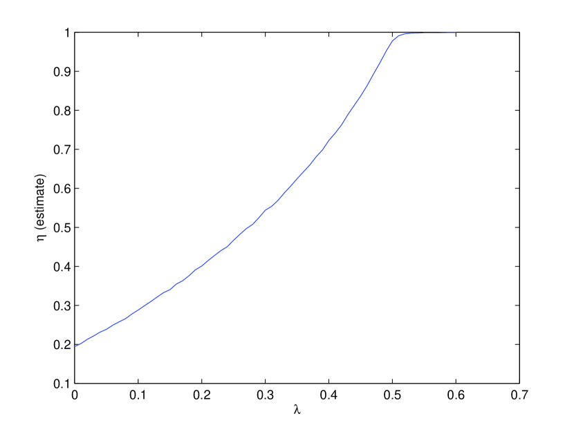
Figure 1. Illustration of Example 3.4.

Proposition 3.3 is proved in Section 4. Our proof of the second part requires taking $E(\Gamma)<1$. It is natural to guess that the condition $\gamma_{0}=0$ in Theorem 1.1 can be replaced by the condition $E(\Gamma)\geq 1$: infections are successful ‘on average’. This is still an open problem, but the following simulation supports this guess.

Example 3.4.

Figure 1 shows estimated values for $\eta(\lambda)$ when $p_{0}=1/4$, $p_{2}=3/4$, $\gamma_{0}=9/20$ and $\gamma_{2}=11/20$. Note that $E(\Gamma)>1$; the simulation suggests that $\eta$ is increasing in $\lambda$. The estimates were obtained by running, for each value of $\lambda$, the process $10^{5}$ times, for $2\cdot 10^{4}$ transitions each. The estimate for $\eta$ is the fraction of runs where $Y$ did not die out. (Usually $Y$ was either 0 or very large at the end of a run.) For reasons similar to the second part of Proposition 3.3, the true value of $\eta(\lambda)$ for $\lambda\geq 0.5$ is 1. However for $\lambda=0.5$ the process $(Y(T_{X}+s))_{s\geq 0}$ is a critical branching process so the time until extinction is large, accounting for the small deviation from 1 in the graph.

3.1. Initial conditions and connection to ODE

Here is a brief informal discussion about how $\eta$ depends on the starting condition $(X(0),Y(0))$ when $\lambda$ and $(\gamma_{k})_{k\geq 0}$ are fixed. We focus on two starting conditions of potential interest, namely $(X(0),Y(0))=(n,1)$ and $(X(0),Y(0))=(n,m)$ where we think of $n$ and $m$ as large, but $n\gg m$. The first situation is where one cell, surrounded by healthy cells, is infected. The second situation would correspond to the case where a large number of healthy cells are encountered by a large number of infected cells. Formal results would be stated asymptotically as $m,n\rightarrow\infty$.

The ‘take-home message’ of Proposition 3.1 is that $(Y(t))_{t\geq 0}$ essentially behaves like a branching process, with a Malthusian parameter that depends on whether $X(t)=0$ or $X(t)>0$. If $X(t)>0$ the Malthusian paramter is $\beta=\alpha+p_{0}E(\Gamma)+\lambda(E(\Gamma)-1)$ as already stated in (7); if $X(t)=0$ the Malthusian parameter is $\beta^{\prime}=\alpha-\lambda$, as is easily deduced from the second part of Proposition 3.1. Here $\alpha=E(\xi)-1$ is as given in (6). Note that $\beta^{\prime}<\beta$.

The most interesting behaviour occurs if $\alpha,\beta>0$, which we assume henceforth. We also assume that $\gamma_{0}>0$, since the case $\gamma_{0}=0$ is easily analyzed using Proposition 3.2 and Theorem 1.1. The main qualitative differences in behaviour occur according as $\beta>\alpha$ or $\beta<\alpha$; in the former case there are two interesting subcases, namely $\beta^{\prime}\leq 0$ and $\beta^{\prime}>0$.

Let us start by considering the initial condition $X(0)=n$, $Y(0)=m$. Since $Y(0)=m$ is large and $\beta>0$, most likely the infected population starts growing. Roughly speaking, $Y(t)\approx me^{\beta t}$. Suppose first $\beta>\alpha$. The healthy population $X(t)$ will then at most be of order $ne^{\alpha t}\ll me^{\beta t}$, and eventually $Y(t)$ will so far exceed $X(t)$ that infections will overwhelm the healthy population, so that we get $X(t_{0})=0$ for some time $t_{0}$. From then on the infected population will have Malthusian parameter $\beta^{\prime}$. If $\beta^{\prime}\leq 0$ this means that $\eta$ will equal 1, whereas if $\beta^{\prime}>0$ then $\eta$ will be close to 0, since $Y(t_{0})$ is large. On the other hand, if $\alpha>\beta$ then typically $X(t)$ will be so much larger than $Y(t)$ that the healthy population does not ‘feel’ the presence of the infection. Since $\beta>0$ and $Y(0)=m$ is large it follows that $\eta$ is close to 0.

Now consider the case $(X(0),Y(0))=(n,1)$. This is similar to the case $(X(0),Y(0))=(n,m)$, except that there is a considerable chance (probability at least $\gamma_{0}(p_{0}+\lambda)/(1+\lambda)$, this being the probability of a lysis leading to no infections) that the infected process dies out in short time. However, if $Y(t)$ does start growing then its size will eventually be in the order of $e^{\beta t}$. From then on the same intuition as for the starting condition $(n,m)$ is valid.

Another way to understand the behaviour described above, in particular the starting condition $(n,m)$, is to look at the ODE model corresponding to our model. Letting $\delta=(p_{0}+\lambda)E(\Gamma)$, this is given by

$$\dot{x}(t)=\alpha x(t)-\delta y(t),\quad\dot{y}(t)=\beta y(t),$$

as long as $x(t)>0$. If $\alpha\neq\beta$ the solution is

$$y(t)=y(0)e^{\beta t},\quad x(t)=\Big{(}x(0)+y(0)\frac{\delta}{\beta-\alpha}\Big{)}e^{\alpha t}-y(0)\frac{\delta}{\beta-\alpha}e^{\beta t}.$$

It is not hard to see that $x(t)$ eventually reaches the absorbing state 0 if $\beta>\alpha$, whereas $x(t)\rightarrow+\infty$ if $\alpha>\beta$ and $x(0)/y(0)=n/m$ is sufficiently large, corresponding to whether the infection takes over or not. We will not study the ODE model further since it cannot give information about survival probabilities.

4. Proofs

In this section we prove Theorem 1.1 and Proposition 3.3. In what follows we will work with two processes $(Z_{i}(t))_{t\geq 0}=(X_{i}(t),Y_{i}(t))_{t\geq 0}$, with parameters $(p_{k})_{k\geq 0}$, $\lambda_{i}$ and $(\gamma^{(i)})_{k\geq 0}$, $i=1,2$, respectively. We write $T_{i}=\inf\{t\geq 0:X_{i}(t)=0\}$.

Theorem 4.1.

Let $0\leq\lambda_{1}\leq\lambda_{2}$, $\gamma^{(1)}\preceq\gamma^{(2)}$, and $\gamma^{(1)}_{0}=\gamma^{(2)}_{0}=0$. Then there is a coupling of the processes $(Z_{i}(t))_{t\geq 0}$ ($i=1,2$) such that the following hold almost surely:

1. $T_{2}\leq T_{1}$,

2. $Y_{2}(t)\geq Y_{1}(t)$ for all $t<T_{2}$,

3. $X_{2}(t)\leq X_{1}(t)$ for all $t\leq T_{2}$, and

4. $X_{1}(t)+Y_{1}(t)\geq X_{2}(t)+Y_{2}(t)$ for all $t\geq 0$.

Before we prove Theorem 4.1, we show how Theorem 1.1 follows, almost immediately, from Theorem 4.1 and Proposition 3.2.

Proof of Theorem 1.1.

By Proposition 3.2 we have $T_{1}<\infty$ almost surely. For $t>T_{1}$ it follows from parts (1) and (4) of Theorem 4.1 that $Y_{1}(t)\geq Y_{2}(t)$, so that $P(Y_{1}(t)\rightarrow 0)\leq P(Y_{2}(t)\rightarrow 0)$. ∎

Proof of Theorem 4.1.

The basic strategy is to ‘twin’ cells in the process $(Z_{1}(t))_{t\geq 0}$ with cells in the process $(Z_{2}(t))_{t\geq 0}$ so that ‘events’ in one process correspond with ‘events’ in the other process. Intuitively, the reason we can acheive a coupling as the one claimed is that only ‘lysis events’ occur at a higher rate in the second process: these events always increase the infected population, but decrease both the healthy and total populations. Here are the details.

It will be convenient to think of $Z_{i}(t)$, $X_{i}(t)$, and $Y_{i}(t)$ ($i=1,2$) as sets of individual cells. Formally, we could label the elements in the set $Z_{i}(t)$ by $(x_{1},i),\ldots(x_{|X_{i}(t)|},i),(y_{1},i),\ldots,(y_{|Y_{i}(t)|},i).$ However, this notation would quickly become cumbersome, and so we will use a somewhat less formal, although still rigorous, approach. We will describe the transitions of the coupled process $(Z_{1}(t),Z_{2}(t))_{t\geq 0}$ at the level of pairs $(a,b)$ of individual cells, where $a\in Z_{1}(t)$ and $b\in Z_{2}(t)$. For each $t\geq 0$, each element of $Z_{1}(t)\cup Z_{2}(t)$ is required to belong to a unique such pair, and we say that $a$ and $b$ are twinned if they belong to the same pair. We allow the possibility $b=\emptyset$, in which case we say that $a$ is untwinned (the possibility $a=\emptyset$ will not occur). We will say that a cell is of type 1 (respectively, type 2) if it belongs to $Z_{1}(t)$ (respectively, $Z_{2}(t)$).

It is a standard consequence of the ordering $\gamma^{(1)}\preceq\gamma^{(2)}$ that we may couple two random variables $\Gamma^{(1)}$ and $\Gamma^{(2)}$ such that $\Gamma^{(1)}$ has law $\gamma^{(1)}$ and $\Gamma^{(2)}$ has law $\gamma^{(2)}$ and $P(\Gamma^{(1)}\leq\Gamma^{(2)})=1$. We assume henceforth that $\{(\Gamma_{1,i},\Gamma_{2,i})\}_{i\geq 1}$ is an i.i.d. sequence such that $\Gamma_{1,i}\leq\Gamma_{2,i}$ for every $i,$ and that $\Gamma_{1,i}$ has law $\gamma^{(1)}$ and $\Gamma_{2,i}$ has law $\gamma^{(2)}.$ In the construction that follows below, if there is a lysis event at some time $\tau,$ we let $I(\tau)$ be the smallest $i$ such that $(\Gamma_{1,i},\Gamma_{2,i})$ has not previously been used in the construction.

We start by describing the coupling $(Z_{1}(t),Z_{2}(t))_{t\geq 0}$ up to time $T_{1}\wedge T_{2}$ (it will transpire that $T_{1}\wedge T_{2}=T_{2}$). It will be convenient to think of healthy cells as coloured blue and infected cells as coloured red. The allowed colour combinations before time $T_{1}\wedge T_{2}$ are the following (the right column introduces notation for the number of pairs of each colour combination):

Colour	Number
$(B,B)$	$b_{2}$
$(R,R)$	$r$
$(B,R)$	$b_{1}$
$(B,\emptyset)$	$b_{0}$

Now we turn to describing the transitions.

1. Any pair $(a,b)$ is replaced by $k\geq 1$ new pairs at rate $p_{k}$; all the new pairs have the same colour combination as the original pair $(a,b)$ (also in the case $b=\emptyset$).

2. A pair of colour $(B,B)$ or $(B,\emptyset)$ is deleted at rate $p_{0}$.

3. A pair $(a,b)=(R,R)$ can give rise to the following additional transitions.

   Firstly, at rate $p_{0}+\lambda_{1}$ it has a type-1-lysis. If $\tau$ is the time of such an event, we first delete $(a,b)$, and then one of the following cases occur.

   Case 1: $\Gamma_{2,I(\tau)}\leq b_{2}$. Then we take $\Gamma_{1,I(\tau)}$ pairs of colour $(B,B)$ and change their colour to $(R,R)$, and we take $\Gamma_{2,I(\tau)}-\Gamma_{1,I(\tau)}$ of the remaining $(B,B)$-pairs and change their colour to $(B,R)$.

   Case 2: $\Gamma_{1,I(\tau)}>b_{2}$. Then we start by changing all the $b_{2}$ pairs of colour $(B,B)$ to $(R,R)$. Let $\Gamma_{1,I(\tau)}^{\prime}:=\Gamma_{1,I(\tau)}-b_{2}>0$, and proceed by changing $\Gamma_{1,I(\tau)}^{\prime}\wedge b_{1}$ pairs of colour $(B,R)$ to colour $(R,R)$. Proceed by letting $\Gamma_{1,I(\tau)}^{{}^{\prime\prime}}:=(\Gamma_{1,I(\tau)}^{\prime}-b_{1})\vee 0$ and changing $\Gamma_{1,I(\tau)}^{{}^{\prime\prime}}\wedge b_{0}$ pairs of colour $(B,\emptyset)$ to $(R,\emptyset)$. Note that in this case we arrive at time $T_{2}\leq T_{1}$, and that this inequality is strict if and only if there remain pairs of colour $(B,R)$ or $(B,\emptyset)$ after the changes are made. In particular, we only create any $(R,\emptyset)$-pairs if we arrive at time $T_{2}$.

   Case 3: $\Gamma_{2,I(\tau)}>b_{2}\geq\Gamma_{1,I(\tau)}$. Then we first take $\Gamma_{1,I(\tau)}$ pairs of colour $(B,B)$ and change their colour to $(R,R)$, and then take the remaining $(b_{2}-\Gamma_{1,I(\tau)})$ pairs of colour $(B,B)$ and change them to $(B,R)$. In this case we arrive at time $T_{2}<T_{1}$.

   Secondly, at rate $\lambda_{2}-\lambda_{1}$ the pair $(a,b)$ has a type-2-lysis. If $\tau$ is the time of such an event:

   (8) $$\begin{array}[]{ccl}&\bullet&\text{the original pair $(a,b)$ stays unaltered;}\\ &\bullet&\text{one pair of colour $(B,B)$ gets replaced by $(B,\emptyset)$;}\\ &\bullet&\text{$(\Gamma_{2,I(\tau)}-1)\wedge(b_{2}-1)$ of the remaining $(b_{2}-1)$ pairs}\\ &&\text{of colour $(B,B)$ have their colour changed to $(B,R)$.}\end{array}$$

   Note that we arrive at time $T_{2}<T_{1}$ if $\Gamma_{2,I(\tau)}\geq b_{2}$.

4. Finally, a pair $(a,b)$ of colour $(B,R)$ can give rise to the following additional transitions,

   Firstly, at rate $p_{0}$ a type-1-death occurs. If $\tau$ is the time of such an event, then $(a,b)$ is deleted and $\Gamma_{2,I(\tau)}\wedge b_{2}$ pairs of colour $(B,B)$ are changed to $(B,R)$. Note that if $\Gamma_{2,I(\tau)}\geq b_{2}$ then we arrive at time $T_{2}<T_{1}$.

   Secondly, at rate $\lambda_{2}$ a type-2-lysis. This yields the exact same transition as described in ( 8). Again, if $\Gamma_{2,I(\tau)}\geq b_{2}$ then we arrive at time $T_{2}<T_{1}$.

It is straightforward to check that the described coupling produces the right marginal dynamics. It might be helpful however to explain why we replace a pair $(B,B)$ by $(B,\emptyset)$ in (8). Here, the cell that lyses is destroyed and one might expect a transition from $(R,R)$ to $(R,\emptyset).$ However, since the type 2 cell that lyses infects cells of $X_{2}(t),$ we pick one of the newly infected type 2 cells (belonging to a $(B,B)$ pair), and twin it with the previous type 1 twin that did not undergo a lysis. The effect is the same as replacing a pair $(B,B)$ by $(B,\emptyset)$ and leaving $(R,R)$ unchanged.

The description above applies until time $T_{2}$; the construction implies that $T_{2}\leq T_{1}$, proving the first part of the theorem. Since a type 1 cell is of colour $R$ only if it is twinned with a type 2 cell of colour $R$ (for $t<T_{2}$), the second part of the theorem also follows. Similarly, a type 2 cell is coloured $B$ only if it is paired with a type 1 cell of colour $B$ (for $t\leq T_{2}$), proving the third part of the theorem.

The construction so far also implies the final part of the theorem for the range $0\leq t\leq T_{2}$ since every type 2 cell has a twin; the construction for $t>T_{2}$, which we will describe now, will preserve this property.

For $t\geq T_{2}$ the process $(Z_{2}(t))_{t\geq T_{2}}$ consists only of infected cells. It will be convenient now to think of the cells of type 2 as green. The reason is that in the absence of healthy cells, the process $(Y_{2}(t))_{t\geq T_{2}}$ evolves differently compared to when $t<T_{2},$ as described above and in Proposition 3.1. Therefore, we keep the colours blue and red for healthy and infected cells of type 1, respectively. At a time $t\geq T_{2}$ we then have the following possible colour combinations (the right column introduces notation for the number of pairs of each colour combination, note that we are redefining $b_{0}$ and $b_{1}$):

Colour	Number
$(B,\emptyset)$	$b_{0}$
$(B,G)$	$b_{1}$
$(R,G)$	$r_{1}$
$(R,\emptyset)$	$r_{0}$

The following transitions may occur.

1. As before, any pair $(a,b)$ is replaced by $k\geq 2$ identical pairs at rate $p_{k}$.

2. A pair of colour $(B,\emptyset)$ or $(B,G)$ is deleted at rate $p_{0}$.

3. A pair of colour $(B,G)$ is, additionally, changed to $(B,\emptyset)$ at rate $\lambda_{2}$.

4. A pair $(a,b)$ of colour $(R,\emptyset)$ or $(R,G)$ lyses at rate $p_{0}+\lambda_{1}$. If $\tau$ is the time of such an event, then we delete $(a,b)$, change the colour of $\Gamma_{1,I(\tau)}^{\prime}=\Gamma_{1,I(\tau)}\wedge b_{0}$ pairs of colour $(B,\emptyset)$ to $(R,\emptyset)$, and finally change the colour of $(\Gamma_{1,I(\tau)}-\Gamma_{1,I(\tau)}^{\prime})\wedge b_{1}$ pairs of colour $(B,G)$ to $(R,G)$.

5. Additionally, a pair of colour $(R,G)$ is replaced by a pair $(R,\emptyset)$ at rate $\lambda_{2}-\lambda_{1}$.

Since a green cell is always twinned with a type 1 cell, this establishes the result.

As before, it is elementary to check that the described coupling produces the right marginal dynamics. ∎

Proof of Proposition 3.3.

For the first part, consider the models where $p_{2}=1$, $0<\lambda<1$ is arbitrary, and where $\gamma^{(1)}_{0}=1$ and $\gamma^{(2)}_{1}=1$. Clearly $\gamma^{(1)}\preceq\gamma^{(2)}$. Write $(X_{1}(t),Y_{1}(t))_{t\geq 0}$ and $(X_{2}(t),Y_{2}(t))_{t\geq 0}$ for the processes with parameters $(p_{k})_{k\geq 0},\lambda,\gamma^{(1)}$ and $(p_{k})_{k\geq 0},\lambda,\gamma^{(2)}$, respectively. Let $X_{1}(0)=X_{2}(0)$ and $Y_{1}(0)=Y_{2}(0).$ There is no interaction between $(X_{1}(t))_{t\geq 0}$ and $(Y_{1}(t))_{t\geq 0}$, and $(Y_{1}(t))_{t\geq 0}$ simply forms a supercritical branching process (this uses $\lambda<1$).

It is straightforward to couple $(Y_{1}(t))_{t\geq 0}$ with $(X_{2}(t),Y_{2}(t))_{t\geq 0}$ so that the following hold. Firstly, each transition $Y_{1}(t)\rightarrow Y_{1}(t)+1$ is accompanied by $(X_{2}(t),Y_{2}(t))\rightarrow(X_{2}(t),Y_{2}(t)+1)$. This simply corresponds to the event that an infected cell is replaced by two identical ones; recall that $p_{2}=1$. Secondly, if $X_{2}(t)\neq 0$ then each transition $Y_{1}(t)\rightarrow Y_{1}(t)-1$ is accompanied by $(X_{2}(t),Y_{2}(t))\rightarrow(X_{2}(t)-1,Y_{2}(t))$. This corresponds to the death of an infected cell: since $\gamma^{(1)}_{0}=1$ such an event simply reduces $Y_{1}(t)$ by $1$, and since $\gamma^{(2)}_{1}=1$ one healthy cell becomes infected in the second process. Thirdly, if $X_{2}(t)=0$ then each transition $Y_{1}(t)\rightarrow Y_{1}(t)-1$ is accompanied by $(X_{2}(t),Y_{2}(t))\rightarrow(X_{2}(t),Y_{2}(t)-1)$. This corresponds to the death of an infected cell in the absence of healthy cells to infect. In such a coupling, $Y_{1}(t)\leq Y_{2}(t)$ for all $t\geq 0$, almost surely, so $\eta(\gamma^{(2)})\leq\eta(\gamma^{(1)})$. It is easy to see that the inequality is in fact strict.

For the second part, we use the result in the forthcoming article [5] that the coexistence probability

$$\zeta(\lambda)=P(X(t)Y(t)\neq 0\;\forall t\geq 0)$$

satisfies: $\zeta=0$ if $\beta\geq\alpha>0$, and $\zeta>0$ if $\alpha>\beta>0$. Note that $\eta<1$ if $\zeta>0$. If $\zeta(\lambda)=0$ and, in addition, $\lambda\geq\alpha$, then it follows from part (2) of Proposition 3.1 that $\eta(\lambda)=1$: either $(Y(t))_{t\geq 0}$ becomes extinct before $(X(t))_{t\geq 0}$, or $(X(t))_{t\geq 0}$ becomes extinct before $(Y(t))_{t\geq 0}$, and in the latter case $(Y(t))_{t\geq 0}$ subsequently forms a branching process which has Malthusian parameter $\beta^{\prime}=\alpha-\lambda\leq 0$ and therefore becomes extinct almost surely. It is easy to check that if $p_{0}=3/8$, $p_{2}=5/8$, $E(\Gamma)=4/5$, $\lambda_{1}=7/8$ and $\lambda_{2}=17/8$, then $\beta(\lambda_{1})=3/8>2/8=\alpha$ and $\lambda_{1}>\alpha$, whereas $\beta(\lambda_{2})=1/8<\alpha$. Thus $\zeta(\lambda_{1})=0$ and $\eta(\lambda_{1})=1$, but $\zeta(\lambda_{2})>0$ so $\eta(\lambda_{2})<1$. ∎

5. Discussion

5.1. Bacteriophage Lambda

The virus Lambda, which preys on the bacterium e-coli, has been the subject of intensive research, mainly to understand the fascinating lysis–lysogeny behaviour [9, 16]. For this virus, a decision between lysis and lysogeny occurs both at the time of infecting a new host, as well as after having been incorporated in the host’s DNA [11]. The switch to lytic behaviour in response to stress to the host seems inevitable [16]. In recent years, some exciting single-cell studies have investigated the factors determining the decision at the time of infection. The results showed strong dependence on environmental signals as well as the volume of the infecting cell and the number of infecting virions per cell (or multiplicity of infection, [8, 21, 22].

A number of mathematical models have been proposed to study the balance between the lytic and lysogenic states [1, 2, 14, 17, 19, 20]. With time the models simulated more and more accurately by including newly discovered genetic components, describing a strict bias towards the lysogenic state as exhibited by ‘wet’ experiments. Both the experimental and theoretical works revealed the molecular mechanism of the decision, but did not study the motivation behind such a strict bias in the decision system, as we do here.

5.2. General conclusion

In this work we have tried to reveal the reason for the observed stability of the lysogenic state. Our results suggest that, regardless of the details of the molecular mechanism behind the decision, the stability of the dormant state is a fundamental part of a long-term survival strategy.

To be specific, in Theorem 1.1 we showed, in the context of our model, not only that $\lambda=0$ maximizes the survival chance $1-\eta(\lambda)$ of the virus, but that $\eta(\lambda)$ is in fact monotonically increasing in $\lambda\geq 0$; this was done under the assumption $\gamma_{0}=0$. Heuristically, monotonicity in $\lambda$ holds for the following reason. As long as $X(t)\neq 0$, the infected process $(Y(t))_{t\geq 0}$ behaves as a branching process with a higher exponential growth rate than $(X(t))_{t\geq 0}$; this follows from Proposition 3.1, equation (7), and the fact that $\gamma_{0}=0$ implies $E(\Gamma)\geq 1$. Typically, therefore, $X(t)=0$ for some $t$, after which point $(Y(t+s))_{s\geq 0}$ by Proposition 3.1 is a branching process with Malthusian parameter $\beta^{\prime}=\alpha-\lambda$ which is decreasing in $\lambda$. The smaller $\lambda$ is, the larger should be the chance that $(Y(t+s))_{s\geq 0}$ survives.

The intuition above is valid whenever $E(\Gamma)\geq 1$, supporting the guess that the conclusion of Theorem 1.1 should hold whenever $E(\Gamma)\geq 1$. We have only been able to make the intuition rigorous when $\gamma_{0}=0$, essentially because then $X(t)\rightarrow 0$ almost surely (by Proposition 3.2), which does not hold if $\gamma_{0}>0$. Interestingly, $\eta(\lambda)$ need not be monotone in $\lambda$ if $E(\Gamma)<1$, as shown in Proposition 3.3; this does not, however, rule out the possibility that $\eta(\lambda)$ still always attains its minimum at $\lambda=0$.

5.3. Decision at the time of infection

The results above concern only the decision between lysis and lysogeny after the virus has been incorporated in the host’s DNA, and not decisions at the time of infection. A simple version of a decision at the time of infection can easily be incorporated into our model as follows.

We modify transition rate (iii) in Section 2.1 so that, with a fixed probability $\kappa>0$, each newly infected cell is immediately replaced by a random (independent) number $\Gamma$ of infected cells, taken from the healthy population $X(t)$. This proceeds recursively for all thereby newly infected cells, until there are either no healthy cells left, or the recursion terminates by itself. Note that the life-length of an infected cell is now a convex combination of an exponential distribution and a Dirac mass at 0, but that the process $(X(t),Y(t))_{t\geq 0}$ is still Markovian. As mentioned, the recursion terminates at the latest when the healthy population $X(t)$ is exhausted. Therefore, there are no transitions of ‘infinite size’.

The total number of new infections due to the original lysis event may be described using a random variable $\Gamma^{\prime}$, whose distribution is easily described in terms of $\kappa,\Gamma$ and $X(t).$ The process thus described is not simply the same as our main model with $\Gamma$ replaced by $\Gamma^{\prime}$ (one easy way to see this is to note that the new process can have transitions decreasing $X(t)+Y(t)$ by more than one at a time). However, it is possible to modify the proofs of Theorems 4.1 and 1.1 to obtain the following:

Theorem 5.1.

In the process with decision at the time of infection described above, with $\gamma_{0}=0$, the extinction probability of $(Y(t))_{t\geq 0}$ is monotonically increasing in $\lambda$, $(\gamma_{k})_{k\geq 0}$ and $\kappa$.

Briefly, the required modifications to Theorem 4.1 are the following; for notation and terminology, see Section 4. In addition to the parameters $\lambda_{1}\leq\lambda_{2}$ and $\gamma^{(1)}\preceq\gamma^{(2)}$ we also have $0\leq\kappa_{1}\leq\kappa_{2}\leq 1$. In the proof of Theorem 4.1 there were several points where pairs of colour $(R,R)$, $(B,R)$, $(R,\emptyset)$ or $(R,G)$ were created. These transitions are still valid, but now, in addition, each newly created $(R,R)$ will itself immediately undergo a type-1-lysis with probability $\kappa_{1}$, or a type-2-lysis with probability $\kappa_{2}-\kappa_{1}$. Similarly, each new $(B,R)$ immediately undergoes a type-2-lysis with probability $\kappa_{2}$, and each new $(R,\emptyset)$ or $(R,G)$ immediately undergoes a lysis with probability $\kappa_{1}$. The same is then done recursively for all thereby newly created pairs $(R,R)$, $(B,R)$, $(R,\emptyset)$ or $(R,G)$. The order in which these ‘immediate’ transitions are carried out is not important. It is easy to see that the conclusions of Theorem 4.1 still hold under these modifications.

Theorem 5.1 says that, when $\gamma_{0}=0$, the optimal ‘choice’ of $\lambda$ and $\kappa$ for the virus is $\lambda=\kappa=0$. Returning to the bacteriophage Lambda, which frequently lyses its host cell immediately after infection, we conclude that the model just described is inadequate as a description of this virus. The main confounding assumptions are presumably: firstly, that $\gamma_{0}=0$; secondly, that there is absolutely no delay between the lytic phase and new infections; and thirdly, that factors such as moi, which experiments have shown to be important, are not included. Furthermore, it is not hard to imagine other factors which could make a more rapid increase in numbers beneficial to the virus in the early stages of an epidemic, such as competition from other viruses or an immune response. It is hoped that relevant modifications of the model can be studied in future work.

5.4. Future directions

The main questions left open by this work are: is Theorem 1.1 true whenever $E(\Gamma)\geq 1$? and, what choices of $\lambda$ and $(\gamma_{k})_{k\geq 0}$ minimize $\eta$ when $E(\Gamma)<1$?

There are many natural ways to modify the model to make it more realistic as a model for viruses. One direction would be to instead let $\Gamma$ be the number of new virions upon a lysis event, and let the number of new infections depends also on the ratio of $X(t)$ to $Y(t)$. Another direction would be to study the model with decision at the moment of infection also when $\gamma_{0}>0$; this requires some new arguments.

It is natural to consider the possibility of two competing viruses, alternatively a virus competing with an immune system. Finally, it would be natural to look at a version of the process which is based not on branching process dynamics, but on the dynamics of population models having some type of equilibrium like the logistic process [18]. Indeed it is reasonable to expect that the cell population will be in equilibrium at the time of infection, possibly making such a formulation closer to reality.

References

- [1] G. K. Ackers, A. D. Johnson, and M. A. Shea. Quantitative model for gene regulation by lambda phage repressor. PNAS, 79(4):1129–1133, 1982.
- [2] A. Arkin, J. Ross, and H.H. McAdams. Stochastic kinetic analysis of developmental pathway bifurcation in phage lambda-infected escherichia coli cells. Genetics, 149:1633–1648, 1998.
- [3] K. B. Athreya and P. Ney. Branching processes. Springer, 1972.
- [4] E. Aurell and K. Sneppen. Epigenetics as a first exit problem. Physical Review Letters, 88:048101, 2002.
- [5] J. E. Björnberg and E. I. Broman. In preparation.
- [6] P. Haccou, P. Jagers, and V. A. Vatutin. Branching processes: variation, growth and extinction of populations. Cambridge University Press, 2005.
- [7] T. E. Harris. The theory of branching processes. Springer, 1963.
- [8] R. I. Joh and J. S. Weitz. To lyse or not to lyse: Transient-mediated stochastic fate determination in cells infected by bacteriophages. PLoS Computational Biology, 7(3), 2011.
- [9] A. D. Johnson, A. R. Poteete, G. Lauer, R. T. Sauer, G. K. Ackers, and M. Ptashne. Lambda repressor and cro—components of an efficient molecular switch. Nature, 294:217–223, 1981.
- [10] W. S. Kendall and I. W. Saunders. Modelling biological populations in space and time. Journal of the Royal Statistical Society B, 45:238–244, 1983.
- [11] M. Lieb. The establishment of lysogenicity in escherichia coli. Journal of Bacteriology, 65:642–651, 1953.
- [12] J. W. Little, D. P. Shepley, and D. W. Wert. Robustness of a gene regulatory circuit. The EMBO Journal, 18:4299–4307, 1999.
- [13] A. Lwoff. Lysogeny. Bacteriological Review, 17(4):269–337, 1953.
- [14] H. H. McAdams and L. Shapiro. Circuit simulation of genetic networks. Science, 269(5224):650–656, 1995.
- [15] M. A. Nowak and R. M. May. Virus dynamics: mathematical principles of immunology and virology. Oxford University Press, 2000.
- [16] A. B. Oppenheim, O. Kobiler, J. Stavans, D. L. Court, and S. Adhya. Switches in bacteriophage lambda development. Annual Review of Genetics, 39:409–429, 2005.
- [17] J. Reinitz and J. R. Vaisnys. Theoretical and experimental analysis of the phage lambda genetic switch implies missing levels of co-operativity. Journal of Theoretical Biology, 145(3):295–318, 1990.
- [18] E. Renshaw. Modelling biological populations in space and time. Cambridge University Press, 1991.
- [19] M. Santillán and M. C. Mackey. Why the lysogenic state of phage lambda is so stable: A mathematical modeling approach. Biophysical Journal, 86(1):75–84, 2004.
- [20] M. A. Shea and G. K. Ackers. The OR control system of bacteriophage lambda. a physical-chemical model for gene regulation. Journal of Molecular Biology, 181(2):211–230, 1985.
- [21] F. St-Perre and D. Endy. Determination of cell fate selection during phage lambda infection. PNAS, 105(52):20705–20710, 2008.
- [22] L. Zeng, S. O. Skinner, C. Zong, J. Sippy, M. Feiss, and I. Golding. Decision making at a subcellular level determines the outcome of bacteriophage infection. Cell, 141(4):682–691, 2010.