The dimension-two gluon condensate, the ghost-gluon vertex and the Taylor theorem

Abstract:

We study the genuine non-perturbative corrections to the Landau gauge ghost-gluon vertex in terms of the non-vanishing dimension-two gluon condensate, and prove these corrections to give account of current SU(2) lattice data for the vertex with different kinematical configurations in the domain of intermediate momenta, roughly above 2-3 GeV. Based on this OPE analysis, we also present a simple model for the vertex, in acceptable agreement with the lattice data also in the IR domain. The necessity of a non-vanishing dimension-two gluon condensate will be also investigated through the analysis of the running coupling defined by the ghost-gluon vertex in Taylor kinematics.

1 Introduction

The infrared properties of the Landau-gauge QCD Green functions have been triggering many studies in the last few years, mainly involving both lattice (see for instance Refs. [1, 2, 3] ) and continuum approaches (see for instance Refs. [4, 5, 6, 7, 8, 9, 10, 11, 12] using Dyson-Schwinger equations (DSE), [13, 14, 15, 16] using the refined Gribov-Zwanziger formalism, [17] using the Curci-Ferrari model as an effective description) or based on the infrared mapping of $\lambda\phi^{4}$ and Yang-Mills teories [18].

Most of the DSE analysis take advantage of approximating the ghost-gluon vertex by a constant when truncating the infinite tower of the relevant equations. To be more precise, only the behaviour of the involved transverse form factor needs to be approximated by a constant for the purpose of truncating the ghost propagator DSE (see also the recent paper [19]). Most of the ammo for the approximation of the ghost-gluon vertex and GPDSE truncation is mainly provided by the Taylor theorem which is widely known as a non-renormalization one [20]. This claims that, in the particular kinematical configurations defined by a vanishing incoming ghost-momentum, no non-zero radiative correction survives for the Landau-gauge ghost-gluon vertex, which takes thus its tree-level expression at any perturbative order [20]. This statement entails two important consequences: that (i) the bare ghost-gluon vertex, defined by

$$\Gamma^{abc}_{\mu}(-q,k;q-k)\ =\ -g_{0}f^{abc}\ \left(\rule[0.0pt]{0.0pt}{14.22636pt}q_{\mu}H_{1}(q,k)+(q-k)_{\mu}H_{2}(q,k)\right)\ ,$$ (1)

is UV-finite for any kinematical configuration; and that (ii) in the specific MOM scheme where the renormalization point is taken with a vanishing incoming ghost momentum (which we named the Taylor scheme –T-scheme– in [21]) the renormalization constant for the ghost-gluon vertex is exactly 1. This allows for a precise lattice determination of the strong running coupling defined in T-scheme  that can be confronted to perturbative prediction in order to estimate $\Lambda_{\overline{\rm MS}}$ [21, 23, 24]. The transverse character of the gluon propagator, in the Landau gauge GPDSE kernel, allows to project out the $H_{2}$-form factor from expression (1). Therefore, we have chosen to call the surviving piece, i.e. $H_{1}$, the transverse form factor. Extending this nomenclature, we call $H_{2}$ the longitudinal vertex form factor.

A precise determination of the ghost dressing function obtained by solving the GPDSE, to be confronted for instance with lattice data, thus requires a correspondingly precise knowledge of the transverse form factor $H_{1}$. To investigate the non-perturbative structure of that form factor was one of main goals of ref. [25], which we will pay attention to in this contribution. That was accomplished, as will be also shown here, by studying the non-perturbative OPE corrections to the perturbative form factor. The non-vanishing dimension-two gluon condensate, $\braket{A^{2}}$, plays a crucial röle for the leading non-perturbative contribution. This condensate was proved not to be neglegible when studying the running of the QCD Green functions [26, 27, 28, 29, 30, 21, 23, 31], but very specially from the analysis of the running of the T-scheme coupling computed by means of lattice simulations with $2+1+1$ twisted-mass dynamical flavours in ref. [32], as will be also shown here.

2 The OPE for the T-scheme running coupling and $\braket{A^{2}}$

A very recent analysis [32] of the strong coupling in T-scheme,

$$\alpha_{T}(q^{2})\ =\ \lim_{\Lambda\to 0}\frac{g_{0}^{2}(\Lambda^{2})}{4\pi}\ G(q^{2},\Lambda^{2})F^{2}(q^{2},\Lambda^{2})\overbrace{\left(H_{1}(q,0)+H_{2}(q,0)\right)}^{\displaystyle=1\ \{\mbox{\rm Taylor theor.}\}}\ ,$$ (2)

where the bare ghost and gluon dressing functions, $G$ and $F$, were computed from lattice simulations with $2+1+1$ twisted-mass dynamical flavours, provided with a very strong evidence for the necessity of applying non-perturbative corrections to account for the running of the coupling,

$$\alpha_{T}(\mu^{2})\ =\ \alpha^{\rm pert}_{T}(\mu^{2})\ \left(1+\frac{9}{\mu^{2}}\ R\left(\alpha^{\rm pert}_{T}(\mu^{2}),\alpha^{\rm pert}_{T}(q_{0}^{2})\right)\left(\frac{\alpha^{\rm pert}_{T}(\mu^{2})}{\alpha^{\rm pert}_{T}(q_{0}^{2})}\right)^{1-\gamma_{0}^{A^{2}}/\beta_{0}}\frac{g^{2}_{T}(q_{0}^{2})\langle A^{2}\rangle_{R,q_{0}^{2}}}{4(N_{C}^{2}-1)}\right)\ ,$$

where $R(\alpha,\alpha_{0})$, $\gamma_{0}^{A^{2}}$ and $\alpha_{T}^{\rm pert}$ can be obtained in perturbation and through the OPE analysis (see ref. [32]). This can be in Fig. 1, borrowed from  [32]. The left plot shows the lattice data for the Taylor coupling multiplied by the square of the momentum plotted in terms of the four-loop perturbative value of the coupling at the same momentum, with a best-fit of $\Lambda_{\overline{\mbox{{\sc ms}}}}$ which gives

$$\alpha_{\overline{\mbox{{\sc ms}}}}(m_{Z})\ =\ 0.1198(9)\ ,$$ (4)

in very good agreement with PDG [33]. One should notice that the departure from zero for the lattice data in the plot can be only explained by non-perturbative contributions and that the Wilson coefficient for the Landau-gauge gluon condensate successfully describes the non-flat behaviour from the data up to $\alpha^{\rm pert}\simeq 0.32$ (the solid line given by Eq. (2)), which roughly corresponds to $p\simeq 3.5$ GeV. The right plot shows the best-fit of Eq. (2) to the lattice data, with a best-fit value of

$$g^{2}(q_{0}^{2})\langle A^{2}\rangle_{R,q_{0}^{2}}\ =\ 4.5(4)\ \mbox{\rm GeV}^{2}\ ,$$ (5)

where $q_{0}^{2}=100$ GeV². These are of course estimates for $\Lambda_{\overline{\mbox{{\sc ms}}}}$ and the gluon condensate including 2 degenerate light quarks and two non-degenerates heavier ones. This allows to run in perturbation the coupling value up to cross safely the bottom mass threshold and run again up to get a “physical” estimate for the coupling at the $Z^{0}$-mass scale, that can be directly (and successfully) compared with experimental results. The same analysis had been previously applied to lattice data in pure Yang-Mills QCD ($N_{f}=0$) [21] and with $N_{f}=2$ twisted-mass dynamical flavours [23], providing with estimates for the gluon condensate slightly depending on the number of light quark flavours, although roughly ranging from 4-6 GeV², when statistical uncertainties are included.

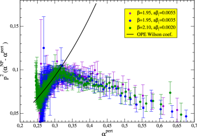
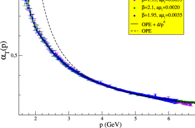
Figure 1: (Left) deviation from the lattice data with respect to the prediction of the four-loop perturbative theory, with the best-fit of $\Lambda_{T}$, plotted in terms of the perturbative running; the solid line shows the leading non-perturbative OPE prediction, Eq. (2.2)’s r.h.s. (Right) The strong running coupling in Taylor scheme defined by Eq. (2.1) obtained over a large momentum range from lattice QCD in ref. [32]. The dotted line stands here for the best-fit with Eq. (2.2), while the solid one includes a higher-order power correction effectively behaving as $\sim 1/p^{6}$.

3 The OPE for the ghost-gluon vertex

We will now pay attention to (and describe with more details) the OPE procedure applied in ref. [25] for the Landau-gauge ghost-gluon vertex,

$$V^{abc}_{\mu}(-q,k;q-k) = \Gamma^{a^{\prime}b^{\prime}c^{\prime}}_{\mu^{\prime}}(-q,k;q-k)\ G^{bb^{\prime}}_{\mu\mu^{\prime}}(q-k)\ F^{aa^{\prime}}(q)\ F^{cc^{\prime}}(k)$$ (6)

$$= \int d^{4}y\ d^{4}x\ e^{i(q-k)\cdot x}\ e^{ik\cdot y}\Braket{\ T\left(c^{c}(y)A^{b}_{\mu}(x)\overline{c}^{a}(0)\right)}$$

is quite similar to the one described in ref. [21]. Here, the OPE expansion shall read

$$V^{abc}_{\mu}(-q,k;q-k) = \left(d_{0}\right)^{abc}_{\mu}(q,k)\$$ (7)

$$+ \left(d_{2}\right)^{abc\mu^{\prime}\nu^{\prime}}_{\mu a^{\prime}b^{\prime}}(q,k)\ \Braket{\ :A_{\mu^{\prime}}^{a^{\prime}}(0)A_{\nu^{\prime}}^{b^{\prime}}(0):}\ +\ \cdots$$

where $d_{0}$ accounts for the purely perturbative contribution to the vertex, while

$$w^{abc}_{\mu} = \left(d_{2}\right)^{abc\mu^{\prime}\nu^{\prime}}_{\mu a^{\prime}b^{\prime}}(q,k)\ \delta^{a^{\prime}b^{\prime}}g_{\mu^{\prime}\nu^{\prime}}$$ (8)

$$= 2I^{[1]}+2I_{s}^{[1]}+2I^{[2]}+4I^{[3]}+2I^{[4]}+I^{[5]}$$

where

$$I^{[1]} =$$ (9)

$$= \rule[0.0pt]{0.0pt}{25.6073pt}\frac{N_{C}}{2}\ g^{2}\ \frac{(q-k)_{\sigma}q_{\sigma}}{q^{2}(q-k)^{2}}\ V^{abc}_{{\rm tree},\mu}(-q,k;q-k)\ ,$$

the tree-level ghost-gluon vertex being

$$V^{abc}_{{\rm tree},\mu}(-q,k;q-k)\ =\ -i\frac{g}{k^{2}q^{2}(q-k)^{2}}\ f^{abc}\ q_{\mu_{2}}\ g^{\perp}_{\mu_{2}\mu}(q-k)\ ,$$ (10)

while

$$I_{s}^{[1]} = \begin{picture}(150.0,45.0)(0.0,0.0) \put(0.0,0.0){} \put(0.0,0.0){} \put(0.0,0.0){} \put(0.0,0.0){} \put(0.0,0.0){} \put(0.0,0.0){} \put(0.0,0.0){} \put(0.0,0.0){} \put(0.0,0.0){} \put(0.0,0.0){} \put(0.0,0.0){} \raise 5.0pt\hbox to0.0pt{\kern 135.0pt\makebox(0.0,0.0)[]{q}\hss} \ignorespaces \raise 5.0pt\hbox to0.0pt{\kern 20.0pt\makebox(0.0,0.0)[]{k}\hss} \ignorespaces \raise 47.0pt\hbox to0.0pt{\kern 125.0pt\makebox(0.0,0.0)[]{q-k}\hss} \ignorespaces \end{picture}\ =\ I^{[1]}\left\{\begin{array}[]{c}q\to-k\\ k\to-q\end{array}\right\}$$ (13)

$$= \rule[0.0pt]{0.0pt}{25.6073pt}-\frac{N_{C}}{2}\ g^{2}\ \frac{(q-k)_{\sigma}k_{\sigma}}{k^{2}(q-k)^{2}}\ V^{abc}_{{\rm tree},\mu}(-q,k;q-k)\,,$$ (14)

and

$$I^{[2]}\rule[0.0pt]{0.0pt}{51.21504pt} =$$ \begin{picture}(120.0,40.0)(0.0,0.0) \put(0.0,0.0){} \put(0.0,0.0){} \put(0.0,0.0){} \put(0.0,0.0){} \put(0.0,0.0){} \put(0.0,0.0){} \put(0.0,0.0){} \put(0.0,0.0){} \put(0.0,0.0){} \put(0.0,0.0){} \end{picture} (15)

$$= \rule[0.0pt]{0.0pt}{22.76228pt}\frac{N_{C}}{4}g^{2}\frac{k_{\sigma}q_{\sigma}}{q^{2}k^{2}}\ V_{{\rm tree},\mu}^{abc}(-q,k;q-k)\ \ .$$

The other contributions, $I^{[3,4,5]}$, can be immediately written using the previous results:

$$I^{[3]}\ = \frac{1}{2}\left(\ \begin{picture}(130.0,25.0)(0.0,0.0) \put(0.0,0.0){} \put(0.0,0.0){} \put(0.0,0.0){} \put(0.0,0.0){} \put(0.0,0.0){} \put(0.0,0.0){} \put(0.0,0.0){} \put(0.0,0.0){} \put(0.0,0.0){} \put(0.0,0.0){} \put(0.0,0.0){} \end{picture}+\begin{picture}(130.0,25.0)(0.0,0.0) \put(0.0,0.0){} \put(0.0,0.0){} \put(0.0,0.0){} \put(0.0,0.0){} \put(0.0,0.0){} \put(0.0,0.0){} \put(0.0,0.0){} \put(0.0,0.0){} \put(0.0,0.0){} \put(0.0,0.0){} \put(0.0,0.0){} \raise 7.0pt\hbox to0.0pt{\kern 10.0pt\makebox(0.0,0.0)[]{k}\hss} \ignorespaces \raise 35.0pt\hbox to0.0pt{\kern 15.0pt\makebox(0.0,0.0)[]{q-k}\hss} \ignorespaces \raise 7.0pt\hbox to0.0pt{\kern 125.0pt\makebox(0.0,0.0)[]{q}\hss} \ignorespaces \end{picture}\ \right)$$ (16)

$$= \left(\frac{N_{C}}{4}\frac{g^{2}}{k^{2}}+\ \frac{N_{C}}{4}\frac{g^{2}}{q^{2}}\right)V_{{\rm tree},\mu}^{abc}(-q,k;q-k)$$

and

$$\rule[0.0pt]{0.0pt}{42.67912pt}2I^{[4]}+I^{[5]}\ = \ 2\times\begin{picture}(120.0,40.0)(0.0,0.0) \put(0.0,0.0){} \put(0.0,0.0){} \put(0.0,0.0){} \put(0.0,0.0){} \put(0.0,0.0){} \put(0.0,0.0){} \put(0.0,0.0){} \put(0.0,0.0){} \put(0.0,0.0){} \put(0.0,0.0){} \put(0.0,0.0){} \put(0.0,0.0){} \end{picture}\ +\begin{picture}(120.0,40.0)(0.0,0.0) \put(0.0,0.0){} \put(0.0,0.0){} \put(0.0,0.0){} \put(0.0,0.0){} \put(0.0,0.0){} \put(0.0,0.0){} \put(0.0,0.0){} \put(0.0,0.0){} \put(0.0,0.0){} \put(0.0,0.0){} \end{picture}$$ (17)

$$= \ N_{C}\frac{g^{2}}{(q-k)^{2}}\ V_{{\rm tree},\mu}^{abc}(-q,k;q-k)$$

In all cases, the blue bubble refers to a contraction of the colour and Lorentz indices with $\frac{1}{2}\delta_{ab}g_{\mu\nu}$. We have also introduced the notation $g^{\perp}_{\mu\nu}(\ell)=g_{\mu\nu}-\frac{\ell_{\mu}\ell_{\nu}}{\ell^{2}}$ for the transverse projector.

Then, one obtains

$$w^{abc}_{\mu}\ =\ g^{2}\ \left(\rule[0.0pt]{0.0pt}{22.76228pt}s_{V}(q,k)+s_{F}(k)+s_{F}(q)+s_{G}(k-q)\right)\,V_{{\rm tree},\mu}^{abc}(-q,k;q-k)$$ (18)

with

$$s_{G}(q) = s_{F}(q)\ =\frac{N_{C}}{q^{2}}\,,$$

$$s_{V}(q,k) = \frac{N_{C}}{2}\left(2\ \frac{(q-k)\cdot q}{q^{2}(q-k)^{2}}+2\ \frac{(k-q)\cdot k}{k^{2}(q-k)^{2}}+\frac{k\cdot q}{k^{2}q^{2}}\right)\,.$$ (19)

$s_{F}$ (resp. $s_{G}$) comes from the OPE corrections to the external ghost (resp. gluon) propagator, i.e. from the non-proper diagrams in Eqs. (16,17) and $s_{V}$ from the proper vertex correction in Eqs. (9,15). The OPE corrections to the proper vertex can be obtained from there, remembering that the bare ghost-gluon vertex reads as:

$$\Gamma^{abc}_{\mu}(-q,k;q-k)\ =\ -g_{0}f^{abc}\ \left(\rule[0.0pt]{0.0pt}{17.07182pt}q_{\mu}H_{1}(q,k)+(q-k)_{\mu}H_{2}(q,k)\right)\ .$$ (20)

Then, in Landau gauge, only the form factor $H_{1}$ survives in the Green function to give:

$$V^{abc}_{\mu}(-q,k;q-k) = -ig_{0}f^{abc}q_{\mu^{\prime}}g^{\perp}_{\mu^{\prime}\mu}(q-k)H_{1}(q,k)\ G((q-k)^{2})\ F(q^{2})\ F(k^{2})\ ,$$ (21)

where $G$ and $F$ are the gluon and ghost dressing functions for which we previously computed the non-perturbative OPE corrections. Thus, one would have:

$$H_{1}(q,k)\ =\ H_{1}^{\rm pert}(q,k)\left(1+s_{V}(q,k)\ \frac{\braket{A^{2}}}{4(N_{C}^{2}-1)}+\ {\cal O}(g^{4},q^{-4},k^{-4},q^{-2}k^{-2})\ \right).$$ (22)

All the non-proper corrections have been removed in the usual way. Now, in order to compare all over the available range of momenta with some current lattice data, we need to try to model the low-momentum behaviour, non-accessible via our previous OPE analysis. This is also done in ref. [25] and will be described in the next section.

4 The Euclidean ghost-gluon vertex and the present lattice data

We will now devote this section to model the transverse form factor of the Euclidean ghost-gluon vertex, $H_{1}$, on the ground provided by Eq. (22), and compare the result with some recent lattice data for this form factor computed in different kinematical configurations.

4.1 The model for the Euclidean ghost-gluon vertex

In Euclidean metrics the bare ghost-gluon vertex can be written very similarly as:

$$\Gamma^{abc}_{{\rm bare},\mu}(-q,k;q-k)\ =\ ig_{0}f^{abc}\ \left(\rule[0.0pt]{0.0pt}{17.07182pt}q_{\mu}H_{1}(q,k)+(q-k)_{\mu}H_{2}(q,k)\right)\,,$$ (23)

where the form factor $H_{1}$ plays a crucial rôle when solving the ghost-propagator Dyson-Schwinger equation (GPDSE) as discussed above. The OPE non-perturbative corrections to the form factor $H_{1}$ were obtained in Eq. (22), but that result is in principle only reliable for large enough $k,q$ and $q-k$ since the SVZ factorization on which it relies might not be valid for low momenta. Nevertheless, in the following we will propose a very simple conjecture to extend Eq. (22) to any momenta, which will provide us with a calculational model for the ghost-gluon vertex to continue research with. In particular, the perturbative part of the ghost-gluon vertex is usually approximated by a constant behaviour; if we then apply a finite renormalization prescription such that

$$\widetilde{Z}_{1}(\mu^{2})\left.H_{1}(q,k)\right|_{\mu^{2}}\ =\ 1\ ,$$ (24)

where the renormalization momentum, $\mu^{2}$, for a given kinematical configuration (for instance, $q-k=0$ and $q^{2}=k^{2}=\mu^{2}$) is chosen to be large enough, on the basis of Eq. (22), we can conjecture that

$$H_{1}(q^{2},k^{2},\theta) = \widetilde{Z}_{1}^{-1}\ \left[\rule[0.0pt]{0.0pt}{27.03003pt}1\ +\ \frac{N_{C}g^{2}\braket{A^{2}}}{8(N_{C}^{2}-1)}\right.$$ (25)

$$\times \left(\frac{\sqrt{k^{2}q^{2}}\cos\theta}{k^{2}q^{2}+m_{\rm IR}^{4}}+\ 2\ \frac{q^{2}-\sqrt{k^{2}q^{2}}\cos\theta}{q^{2}(q^{2}+k^{2}-2\sqrt{q^{2}k^{2}}\cos\theta)+m_{\rm IR}^{4}}\right.$$

$$\left.\left.+\ 2\ \frac{k^{2}-\sqrt{k^{2}q^{2}}\cos\theta}{k^{2}(q^{2}+k^{2}-2\sqrt{q^{2}k^{2}}\cos\theta)+m_{\rm IR}^{4}}\right)\rule[0.0pt]{0.0pt}{27.03003pt}\right]\ ,$$

gives a reasonable description of the ghost-gluon form factor $H_{1}$ all over the range of its momenta $q$ and $k$, where $\theta$ stands for the angle between them. The purpose of Eq. (25) is to keep the main features of the momentum behaviour of the ghost-gluon form factor provided by the OPE analysis and to give a rough description of the deep IR only with the introduction of some IR mass scale, $m_{\rm IR}$, that can be thought as some sort of IR regulator (related to some kind of effective gluon mass) and which is mainly aimed to avoid the spurious singularities resulting from the OPE expansion in momentum inverse powers.

Of course, $\mu^{2}$ being large enough, $\widetilde{Z}_{1}$ can be approximated by some constant value for any $\mu^{2}$ because the logarithmic behaviour of the ghost-gluon in perturbation theory has been proven to be very smooth [36, 37]. Thus Eq. (25) provides us with a very economical model because one needs nothing but some infrared mass parameter which, being related to the gluon mass, is expected to be $\sim 1$ GeV, to parametrize the deep infrared behaviour of the ghost-gluon transverse form factor. It should be noted that, although the ghost-gluon vertex form factors do not diverge, the gluon condensate does: it is the product of the Wilson coefficient and of the condensate which is expected to remain finite thanks to a delicate compensation of singularities, in the sum-rules approach. Then, both the Wilson coefficient and the condensate should be renormalized, by fixing some particular prescription, and both shall depend on a chosen renormalization momentum. This is explained in detail in the work of ref. [31] where the Wilson coefficient for the quark propagator is included at order ${\cal O}(\alpha^{4})$. Since we carry out the computation of the Wilson coefficient in Eqs. (9-17) only at tree-level and neglect its logarithmic dependence, we do not specify any renormalization momentum for the gluon condensate.

4.2 Comparing with available lattice data

Some SU(2) and SU(3) lattice results for the ghost-gluon vertex are available in the literature (see for instance Refs. [34, 35]). In particular, Cucchieri et al. have computed the tree-level-tensor form factor in SU(2) for three kinematics ($p\equiv q-k$ is the gluon momentum and $\varphi$ the angle between the gluon and ghost momenta) : (1) $p^{2}=q^{2}$ and $\varphi=\pi/2$, (2) $p^{2}=0$ and (3) $\varphi=\pi/3$ with $p^{2}=q^{2}=k^{2}$ ([34]). As can be seen in the left pane of Fig. 2, when we plug $g^{2}\langle A^{2}\rangle=6$ GeV², $m_{\rm IR}=1.4$ GeV and $\widetilde{Z}_{1}^{-1}=1.04$ into Eq. (25), the prediction for the form factor $H_{1}$ appears to agree pretty well with the SU(2) lattice data for the three kinematical configurations above mentioned. It should be also noted that the OPE prediction without the infrared completion through the introduction of $m_{\rm IR}$ given by Eqs. (3,22), plotted with dotted lines, also accounts very well for lattice data in the intermediate momenta region, above roughly $2.5$ GeV. Furthermore, the value for the gluon condensate lies in the same ballpark as the estimates obtained from the SU(3) analysis of the Taylor coupling in ref. [21]. This strongly supports that the OPE analysis indeed captures the kinematical structure for the form factor $H_{1}$. On the other hand, the infrared mass scale, as supposed, is of the order of 1 GeV and the (very close to 1) value for $\widetilde{Z}_{1}^{-1}$ accounts reasonably for perturbative value of $H_{1}$ that we approximated by a constant. Thus, after paying the economical price of incorporating only these two more parameters, both taking also reasonable values, we are left with a reliable closed formula for the form factor at any gluon or ghost momenta. This is a very useful ingredient for the numerical integration of the GPDSE.

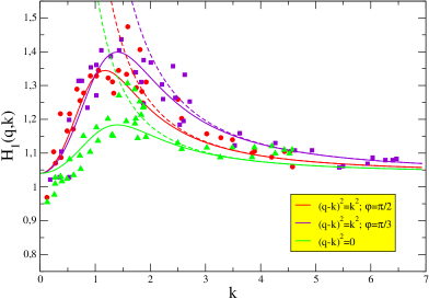
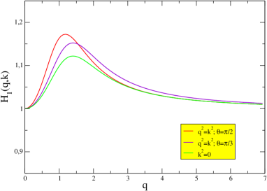
Figure 2: (left) The predictions of the model for $H_{1}$ (solid lines) in Eq. (4.3) and the OPE result without infrared completion (dotted lines) in Eq. (3.14) confronted to the SU(2) lattice data borrowed from ref. [34] for the three kinematical configurations described in the main text: $(k-q)^{2}=q^{2}$ for $\varphi=\pi/3$ (violet) and $\varphi=\pi/2$ (red) and $(k-q)^{2}=0$ (green). (right) The results of the model for $H_{1}$ in the SU(3) case and for the following kinematical configurations: $k^{2}=q^{2}$ for $\theta=\pi/3$ (violet) and $\theta=\pi/2$ (red) and $k^{2}=0$ (green).

The SU(3) results published by the authors of ref. [35] appear to be very noisy and cannot be invoked to properly discriminate whether a constant behaviour close to 1 or Eq. (25) accounts better for them. However, we can now take the mass parameter, $m_{\rm IR}$, from the previous SU(2) analysis and the well-known SU(3) value for $g^{2}\braket{A^{2}}$, assume $\widetilde{Z}_{1}^{-1}=1$ and use Eq. (25) to predict the ghost-gluon transverse form factor, $H_{1}$. This is shown in the right plot of in Fig. 2 for three different kinematical configurations and, as can be seen, the deviations from 1 appear to be very small in all the cases and compatible with the results shown in Fig. 4 of ref. [35] for the vanishing gluon momentum case.

4.3 The Taylor kinematics and the asymmetric gluon-ghost vertex

The kinematical configuarition where the incoming ghost momentum goes to zero ($k\to 0$) is especially interesting, as this is the one which one defines the T-scheme for (as shown in sec.2). Let us pay some additional attention to it. In this particular kinematical limit, it is exactly obtained up to all perturbative orders:

$$\Gamma^{abc}_{{\rm bare},\mu}(-q,0;q)\ =\ -gf^{abc}q_{\mu}\ .$$ (26)

At any order of perturbation theory, this implies that $H_{1}(q,0)+H_{2}(q,0)=1$. According to Eq. (25), one would have

$$H_{1}(q,0)\ =\ \widetilde{Z}_{1}^{-1}\ \left(1+N_{C}\frac{g^{2}\braket{A^{2}}}{4(N_{C}^{2}-1)}\ \frac{q^{2}}{q^{4}+m_{IR}^{4}}\ \right)\ .$$ (27)

An interesting question to investigate is whether such a genuine non-perturbative correction still survives for the full ghost-gluon vertex in the Taylor limit, and not only for the transverse form factor $H_{1}$. Said otherwise, does eq.(26) maintains its validity upon adding the OPE corrections related to $\braket{A^{2}}$ to it, or not? This question have been properly addressed in ref. [25], where the asymmetric ghost-gluon vertex is studied and one is left with

$$\Gamma^{abc}_{\mu}(-q,\varepsilon;q-\varepsilon)\ =\ -gf^{abc}\left(\rule[0.0pt]{0.0pt}{17.07182pt}q_{\mu}\ H_{1}(q,\varepsilon)\ +\ (q-\varepsilon)_{\mu}\ H_{2}(q,\varepsilon)\right)\ +\ \cdots$$ (28)

where

$$H_{1}(q,\varepsilon) = H_{1}^{\rm pert}(q,\varepsilon)\ +\ N_{C}\ g^{2}\frac{(q-\varepsilon)\cdot q}{q^{2}(q-\varepsilon)^{2}}\ \frac{\braket{A^{2}}}{4(N^{2}_{C}-1)}\ ,$$

$$H_{2}(q,\varepsilon) = H_{2}^{\rm pert}(q,\varepsilon)\ -\ N_{C}\ g^{2}\ \frac{\left((q-\varepsilon)\cdot q\right)^{2}}{q^{2}(q-\varepsilon)^{4}}\ \frac{\braket{A^{2}}}{4(N^{2}_{C}-1)}\ .$$ (29)

Thus, after taking the limit $\varepsilon\to 0$, one will have:

$$\Gamma^{abc}_{\mu}(-q,0;q)\ =\ -gf^{abc}\ q_{\mu}\left(\ \rule[0.0pt]{0.0pt}{17.07182pt}H_{1}^{\rm pert}(q,0)\ +\ H_{2}^{\rm pert}(q,0)\ \right)\ =\ -gf^{abc}\ q_{\mu}\ .$$ (30)

Thus, the result applied in Eq. (2) to define the T-scheme coupling is recovered. This confirms that no non-perturbative OPE correction survives in the proper ghost-gluon vertex in the Taylor limit, although both form factors $H_{1}$ and $H_{2}$ separately undergo such a kind of correction.

5 Conclusions

The momentum behaviour of the ghost-gluon vertex has been studied in the framework of the operator product expansion (OPE). This approach has already been proved in the literature to be very fruitful in describing the running of two-point gluon and quark Green functions and of the strong coupling computed in several MOM renormalization schemes. In particular, the coupling derived from the ghost-gluon vertex renormalized in T-scheme, which can be directly computed from nothing else but the ghost and gluon propagators, led to a very accurate determination of $\Lambda_{\rm QCD}$ when its running with momenta obtained from the lattice estimate has been confronted with the OPE prediction, although only after accounting properly for a dimension-two gluon condensate, $\braket{A^{2}}$. The same approach is followed to study the ghost-gluon vertex and special attention is payed to the transverse form factor for the ghost-gluon vertex, precisely the one that plays a crucial rôle for the truncation and resolution of the GPDSE and that, in this context, is usually approximated by a constant. In this way, a genuine non-perturbative OPE correction to the perturbative part for the transverse form factor is obtained. A very simple conjecture, made to extend the OPE description beyond the momentum range where the SVZ factorization is supposed to work, left us with a simple model describing the momentum behaviour of the ghost-gluon form factor. This model was shown to agree pretty well with a lattice SU(2) computation for several kinematical configurations of the ghost-gluon vertex, when the value for the gluon condensate is in the same ballpark as the one that is estimated from the running of the T-scheme coupling in SU(3) lattice gauge theory. This successful comparison with the available lattice data provides us with strong indications that (i) the OPE framework helps to account for the kinematical structure of the ghost-gluon vertex at intermediate momentum domain and (ii) that it helps to cook up a reliable model, providing a good parameterization also for the IR domain, to be plugged into the GPDSE to reproduce the ghost propagator lattice data. Finally, we also proved that, in the particular kinematical limit associated with the Taylor theorem and hence by the T-scheme (a vanishing incoming ghost momentum), the corrections to the longitudinal and transverse form factors cancel against each other and that the tree-level result for the ghost-gluon vertex is thus recovered.

Acknowledgements: J. R-Q acknowledges the Spanish MICINN for the support by the research project FPA2009-10773 and “Junta de Andalucia” by P07FQM02962.

References

- [1] A. Cucchieri and T. Mendes, Phys.Rev.Lett. 100 (2008) 241601, arXiv:0712.3517 [hep-lat]. Phys.Rev. D78 (2008) 094503, arXiv:0804.2371 [hep-lat]. Phys.Rev. D81 (2010) 016005, arXiv:0904.4033 [hep-lat].
- [2] P. Costa, O. Oliveira, and P. Silva, Phys.Lett. B695 (2011) 454–458, arXiv:1011.5603 [hep-ph]. O. Oliveira and P. Bicudo, J.Phys.G G38 (2011) 045003, arXiv:1002.4151 [hep-lat].
- [3] I. Bogolubsky, V. Bornyakov, G. Burgio, E. Ilgenfritz, M. Muller-Preussker, et al., Phys.Rev. D77 (2008) 014504, arXiv:0707.3611 [hep-lat]. I. Bogolubsky, E. Ilgenfritz, M. Muller-Preussker, and A. Sternbeck, Phys.Lett. B676 (2009) 69–73, arXiv:0901.0736 [hep-lat]. V. G. Bornyakov, V. K. Mitrjushkin, and M. Muller-Preussker, Phys. Rev. D81 (2010) 054503, arXiv:0912.4475 [hep-lat].
- [4] A. C. Aguilar, D. Binosi, and J. Papavassiliou, Phys. Rev. D78 (2008) 025010, arXiv:0802.1870 [hep-ph].
- [5] D. Binosi and J. Papavassiliou, Phys.Rept. 479 (2009) 1–152, arXiv:0909.2536 [hep-ph].
- [6] P. Boucaud, J. Leroy, A. Le Yaouanc, J. Micheli, O. Pène, et al., JHEP 0806 (2008) 099, arXiv:0803.2161 [hep-ph].
- [7] P. Boucaud, J.-P. Leroy, A. Yaouanc, J. Micheli, O. Pène, et al., JHEP 0806 (2008) 012, arXiv:0801.2721 [hep-ph].
- [8] P. Boucaud, M. Gomez, J. Leroy, A. Le Yaouanc, J. Micheli, et al., Phys.Rev. D82 (2010) 054007, arXiv:1004.4135 [hep-ph].
- [9] J. Rodriguez-Quintero, JHEP 1101 (2011) 105, arXiv:1005.4598 [hep-ph].
- [10] C. S. Fischer, A. Maas, and J. M. Pawlowski, Annals Phys. 324 (2009) 2408–2437, arXiv:0810.1987 [hep-ph].
- [11] C. S. Fischer and J. M. Pawlowski, Phys. Rev. D80 (2009) 025023, arXiv:0903.2193 [hep-th].
- [12] R. Alkofer, M. Q. Huber, and K. Schwenzer, Phys.Rev. D81 (2010) 105010, arXiv:0801.2762 [hep-th].
- [13] D. Dudal, R. Sobreiro, S. Sorella, and H. Verschelde, Phys.Rev. D72 (2005) 014016, arXiv:hep-th/0502183 [hep-th].
- [14] D. Dudal, S. Sorella, N. Vandersickel, and H. Verschelde, Phys.Rev. D77 (2008) 071501, arXiv:0711.4496 [hep-th].
- [15] D. Dudal, J. A. Gracey, S. P. Sorella, N. Vandersickel, and H. Verschelde, Phys.Rev. D78 (2008) 065047, arXiv:0806.4348 [hep-th].
- [16] D. Dudal, O. Oliveira, and N. Vandersickel, Phys.Rev. D81 (2010) 074505, arXiv:1002.2374 [hep-lat].
- [17] M. Tissier and N. Wschebor, Phys.Rev. D82 (2010) 101701, arXiv:1004.1607 [hep-ph]. Phys.Rev. D84 (2011) 045018, arXiv:1105.2475 [hep-th].
- [18] M. Frasca, Phys.Lett. B670 (2008) 73–77, arXiv:0709.2042 [hep-th]. Nucl. Phys. Proc. Suppl. 186 (2009) 260–263, arXiv:0807.4299 [hep-ph].
- [19] M. R. Pennington and D. J. Wilson, arXiv:1109.2117 [hep-ph].
- [20] J. Taylor, Nucl.Phys. B33 (1971) 436–444.
- [21] P. Boucaud, F. De Soto, J. Leroy, A. Le Yaouanc, J. Micheli, O. Pène, and J. Rodríguez-Quintero, Phys.Rev. D79 (2009) 014508, arXiv:0811.2059 [hep-ph].
- [22] A. C. Aguilar, D. Binosi, J. Papavassiliou, and J. Rodriguez-Quintero, Phys. Rev. D80 (2009) 085018, arXiv:0906.2633 [hep-ph].
- [23] ETM Collaboration, B. Blossier et al., Phys. Rev. D82 (2010) 034510, arXiv:1005.5290 [hep-lat].
- [24] A. Sternbeck et al., PoS LAT2009 (2009) 210, arXiv:1003.1585.
- [25] P. Boucaud, D. Dudal, J. Leroy, O. Pene, and J. Rodriguez-Quintero, arXiv:1109.3803 [hep-ph].
- [26] P. Boucaud, A. Le Yaouanc, J. Leroy, J. Micheli, O. Pène, and J. Rodríguez-Quintero, Phys.Lett. B493 (2000) 315–324, arXiv:hep-ph/0008043 [hep-ph].
- [27] P. Boucaud et al., JHEP 01 (2002) 046, arXiv:hep-ph/0107278.
- [28] P. Boucaud, A. Le Yaouanc, J. Leroy, J. Micheli, O. Pène, and J. Rodríguez-Quintero, Phys.Rev. D63 (2001) 114003, arXiv:hep-ph/0101302 [hep-ph].
- [29] F. De Soto and J. Rodriguez-Quintero, Phys.Rev. D64 (2001) 114003, arXiv:hep-ph/0105063 [hep-ph].
- [30] P. Boucaud, J. Leroy, A. Le Yaouanc, A. Lokhov, J. Micheli, et al., JHEP 0601 (2006) 037, arXiv:hep-lat/0507005 [hep-lat].
- [31] B. Blossier et al., Phys. Rev. D83 (2011) 074506, arXiv:1011.2414 [hep-ph].
- [32] B. Blossier, P. Boucaud, M. Brinet, F. De Soto, X. Du, et al., arXiv:1110.5829 [hep-lat].
- [33] Particle Data Group Collaboration, K. Nakamura et al., “Review of particle physics,” J. Phys. G37 (2010) 075021.
- [34] A. Cucchieri, A. Maas, and T. Mendes, Phys.Rev. D77 (2008) 094510, arXiv:0803.1798 [hep-lat].
- [35] A. Sternbeck, E.-M. Ilgenfritz, M. Muller-Preussker, and A. Schiller, Nucl.Phys.Proc.Suppl. 153 (2006) 185–190, arXiv:hep-lat/0511053 [hep-lat].
- [36] K. Chetyrkin and A. Retey, arXiv:hep-ph/0007088 [hep-ph].
- [37] A. I. Davydychev, P. Osland, and O. Tarasov, Phys.Rev. D54 (1996) 4087–4113, arXiv:hep-ph/9605348 [hep-ph].
- [38] W. Schleifenbaum, A. Maas, J. Wambach, and R. Alkofer, Phys. Rev. D72 (2005) 014017, arXiv:hep-ph/0411052.