Initial conditions for dipole evolution
beyond the McLerran-Venugopalan model
Adrian Dumitrua,b,c b,c
a b c
Abstract
We derive the scattering amplitude N ( r ) 𝑁 𝑟 N(r) ∼ ρ 4 similar-to absent superscript 𝜌 4 \sim\rho^{4} x 𝑥 x N ( r ) 𝑁 𝑟 N(r) et al. over a broad range of dipole
sizes r 𝑟 r A 𝐴 A N ( r ) 𝑁 𝑟 N(r) A 𝐴 A bremsstrahlung tail.
† † preprint: RBRC-935
In this paper we derive the dipole scattering amplitude
N ( r ) 𝑁 𝑟 N(r) Mueller:1993rr r 𝑟 r ∼ ρ 4 similar-to absent superscript 𝜌 4 \sim\rho^{4} x 𝑥 x
Our result may prove useful for a better theoretical understanding of
the A 𝐴 A N ( r ) 𝑁 𝑟 N(r)
Let us first recall the setup for the McLerran-Venugopalan (MV)
model MV x 𝑥 x ρ a ( x ⟂ , x − ) superscript 𝜌 𝑎 subscript 𝑥 perpendicular-to superscript 𝑥 \rho^{a}(x_{\perp},x^{-}) x − superscript 𝑥 x^{-} ρ 𝜌 \rho ρ 𝜌 \rho
S M V [ ρ ] = ∫ d 2 𝕩 ⟂ ∫ − ∞ ∞ 𝑑 x − ρ a ( x − , 𝕩 ⟂ ) ρ a ( x − , 𝕩 ⟂ ) 2 μ 2 ( x − ) . subscript 𝑆 𝑀 𝑉 delimited-[] 𝜌 superscript 𝑑 2 subscript 𝕩 perpendicular-to subscript superscript differential-d superscript 𝑥 superscript 𝜌 𝑎 superscript 𝑥 subscript 𝕩 perpendicular-to superscript 𝜌 𝑎 superscript 𝑥 subscript 𝕩 perpendicular-to 2 superscript 𝜇 2 superscript 𝑥 \displaystyle S_{MV}[\rho]=\int d^{2}\mathbb{x}_{\perp}\int^{\infty}_{-\infty}dx^{-}~{}\frac{\rho^{a}(x^{-},\mathbb{x}_{\perp})\,\rho^{a}(x^{-},\mathbb{x}_{\perp})}{2\mu^{2}(x^{-})}~{}. (1)
Here, μ 2 ( x − ) d x − superscript 𝜇 2 superscript 𝑥 𝑑 superscript 𝑥 \mu^{2}(x^{-})dx^{-} x − superscript 𝑥 x^{-} x − + d x − superscript 𝑥 𝑑 superscript 𝑥 x^{-}+dx^{-}
∫ − ∞ ∞ 𝑑 x − μ 2 ( x − ) ∼ g 2 A 1 / 3 similar-to superscript subscript differential-d superscript 𝑥 superscript 𝜇 2 superscript 𝑥 superscript 𝑔 2 superscript 𝐴 1 3 \int_{-\infty}^{\infty}dx^{-}\mu^{2}(x^{-})\sim g^{2}A^{1/3} (2)
is proportional to the thickness ∼ A 1 / 3 similar-to absent superscript 𝐴 1 3 \sim A^{1/3}
D ( r ) 𝐷 𝑟 \displaystyle D(r) ≡ \displaystyle\equiv 1 N c ⟨ tr V ( 𝕩 ⟂ ) V † ( 𝕪 ⟂ ) ⟩ 1 subscript 𝑁 𝑐 delimited-⟨⟩ tr 𝑉 subscript 𝕩 perpendicular-to superscript 𝑉 † subscript 𝕪 perpendicular-to \displaystyle\frac{1}{N_{c}}\langle\mathrm{tr}~{}V(\mathbb{x}_{\perp})V^{\dagger}(\mathbb{y}_{\perp})\rangle (3)
= \displaystyle= exp ( − g 4 C F 8 π ∫ 𝑑 x − μ 2 ( x − ) r 2 log 1 r Λ ) superscript 𝑔 4 subscript 𝐶 𝐹 8 𝜋 differential-d superscript 𝑥 superscript 𝜇 2 superscript 𝑥 superscript 𝑟 2 1 𝑟 Λ \displaystyle\exp\left(-\frac{g^{4}C_{F}}{8\pi}\int dx^{-}\mu^{2}(x^{-})~{}r^{2}\log\frac{1}{r\Lambda}\right) (4)
= \displaystyle= exp ( − Q s 2 r 2 4 log 1 r Λ ) , superscript subscript 𝑄 𝑠 2 superscript 𝑟 2 4 1 𝑟 Λ \displaystyle\exp\left(-\frac{Q_{s}^{2}\,r^{2}}{4}\log\frac{1}{r\Lambda}\right)~{}, (5)
where r ≡ | 𝕩 ⟂ − 𝕪 ⟂ | 𝑟 subscript 𝕩 perpendicular-to subscript 𝕪 perpendicular-to r\equiv|\mathbb{x}_{\perp}-\mathbb{y}_{\perp}| Λ Λ \Lambda r 𝑟 r log 1 / ( r Λ ) ≫ 1 much-greater-than 1 𝑟 Λ 1 \log 1/(r\Lambda)\gg 1 Q s subscript 𝑄 𝑠 Q_{s} JalilianMarian:1996xn ; hep-ph/9802440 ; GelisPeshier
To go beyond the limit of infinite valence charge density one
considers a “random walk” in the space of SU(3) representations
constructed from the direct product of a large number of fundamental
charges JV arXiv:1105.4155
S [ ρ ] = ∫ d 2 𝕧 ⟂ ∫ − ∞ ∞ d v 1 − { ρ a ( v 1 − , 𝕧 ⟂ ) ρ a ( v 1 − , 𝕧 ⟂ ) 2 μ 2 ( v 1 − ) − d a b c ρ a ( v 1 − , 𝕧 ⟂ ) ρ b ( v 1 − , 𝕧 ⟂ ) ρ c ( v 1 − , 𝕧 ⟂ ) κ 3 \displaystyle S[\rho]=\int d^{2}\mathbb{v}_{\perp}\int^{\infty}_{-\infty}dv_{1}^{-}\left\{\frac{\rho^{a}(v_{1}^{-},\mathbb{v}_{\perp})\rho^{a}(v_{1}^{-},\mathbb{v}_{\perp})}{2\mu^{2}(v_{1}^{-})}-\frac{d^{abc}\rho^{a}(v_{1}^{-},\mathbb{v}_{\perp})\rho^{b}(v_{1}^{-},\mathbb{v}_{\perp})\rho^{c}(v_{1}^{-},\mathbb{v}_{\perp})}{\kappa_{3}}\right.
+ ∫ − ∞ ∞ d v 2 − ρ a ( v 1 − , 𝕧 ⟂ ) ρ a ( v 1 − , 𝕧 ⟂ ) ρ b ( v 2 − , 𝕧 ⟂ ) ρ b ( v 2 − , 𝕧 ⟂ ) κ 4 } . \displaystyle\left.+\int^{\infty}_{-\infty}dv_{2}^{-}\,\frac{\rho^{a}(v_{1}^{-},\mathbb{v}_{\perp})\rho^{a}(v_{1}^{-},\mathbb{v}_{\perp})\rho^{b}(v_{2}^{-},\mathbb{v}_{\perp})\rho^{b}(v_{2}^{-},\mathbb{v}_{\perp})}{\kappa_{4}}\right\}~{}. (6)
The coefficients of the higher dimensional operators are
κ 3 subscript 𝜅 3 \displaystyle\kappa_{3} ∼ similar-to \displaystyle\sim g 3 A 2 / 3 , superscript 𝑔 3 superscript 𝐴 2 3 \displaystyle g^{3}A^{2/3}~{}, (7)
κ 4 subscript 𝜅 4 \displaystyle\kappa_{4} ∼ similar-to \displaystyle\sim g 4 A , superscript 𝑔 4 𝐴 \displaystyle g^{4}A~{}, (8)
and so involve higher powers of g A 1 / 3 𝑔 superscript 𝐴 1 3 gA^{1/3} κ 4 subscript 𝜅 4 \kappa_{4} ∼ ρ 3 similar-to absent superscript 𝜌 3 \sim\rho^{3} 6 1 / κ 3 1 subscript 𝜅 3 1/\kappa_{3} T 𝑇 T
N ( r ) 𝑁 𝑟 \displaystyle N(r) ≡ \displaystyle\equiv 1 − D ( r ) 1 𝐷 𝑟 \displaystyle 1-D(r) (9)
= \displaystyle= Q s 2 r 2 4 log 1 r Λ − C F 2 6 π 3 g 8 κ 4 [ ∫ − ∞ ∞ 𝑑 z − μ 4 ( z − ) ] 2 r 2 log 3 1 r Λ , ( r 2 Q s 2 < 1 ) . superscript subscript 𝑄 𝑠 2 superscript 𝑟 2 4 1 𝑟 Λ superscript subscript 𝐶 𝐹 2 6 superscript 𝜋 3 superscript 𝑔 8 subscript 𝜅 4 superscript delimited-[] superscript subscript differential-d superscript 𝑧 superscript 𝜇 4 superscript 𝑧 2 superscript 𝑟 2 superscript 3 1 𝑟 Λ superscript 𝑟 2 superscript subscript 𝑄 𝑠 2 1
\displaystyle\frac{Q_{s}^{2}r^{2}}{4}\log\frac{1}{r\Lambda}-\frac{C_{F}^{2}}{6\pi^{3}}\frac{g^{8}}{\kappa_{4}}\left[\int_{-\infty}^{\infty}dz^{-}\mu^{4}(z^{-})\right]^{2}r^{2}\log^{3}\frac{1}{r\Lambda}~{}~{}~{},~{}~{}~{}(r^{2}Q_{s}^{2}<1)~{}.
This now involves a new moment of the valence color charge
distribution, namely ∫ 𝑑 x − μ 4 ( x − ) differential-d superscript 𝑥 superscript 𝜇 4 superscript 𝑥 \int dx^{-}\mu^{4}(x^{-}) 𝒪 ( 1 / κ 4 ) 𝒪 1 subscript 𝜅 4 \mathcal{O}(1/\kappa_{4}) ∼ r 2 similar-to absent superscript 𝑟 2 \sim r^{2} 1 6 r ∼ > 1 / Q s superscript similar-to 𝑟 1 subscript 𝑄 𝑠 r\,\,\vbox{\hbox{$\buildrel\displaystyle>\over{\sim}$}}\,\,1/Q_{s} ρ a ( x − , 𝕩 ⟂ ) superscript 𝜌 𝑎 superscript 𝑥 subscript 𝕩 perpendicular-to \rho^{a}(x^{-},\mathbb{x}_{\perp}) Lappi:2007ku
The dipole scattering amplitude for a proton target has been fitted in
ref. AAMQS x 𝑥 x
N AAMQS ( r , x 0 = 0.01 ) = 1 − exp [ − 1 4 ( r 2 Q s 2 ( x 0 ) ) γ log ( e + 1 r Λ ) ] , subscript 𝑁 AAMQS 𝑟 subscript 𝑥 0
0.01 1 1 4 superscript superscript 𝑟 2 superscript subscript 𝑄 𝑠 2 subscript 𝑥 0 𝛾 𝑒 1 𝑟 Λ N_{\rm AAMQS}(r,x_{0}=0.01)=1-\exp\left[-\frac{1}{4}\left(r^{2}Q_{s}^{2}(x_{0})\right)^{\gamma}\log\left(e+\frac{1}{r\Lambda}\right)\right]~{}, (10)
with γ ≃ 1.119 similar-to-or-equals 𝛾 1.119 \gamma\simeq 1.119 simultaneously provides a good description of charged hadron
transverse momentum distributions in p + p 𝑝 𝑝 p+p pp_ptDistr 5 p ⟂ ∼ > 6 superscript similar-to subscript 𝑝 perpendicular-to 6 p_{\perp}\,\,\vbox{\hbox{$\buildrel\displaystyle>\over{\sim}$}}\,\,6 pp_ptDistr
However, since the model (10 R p A subscript 𝑅 𝑝 𝐴 R_{pA} p + P b 𝑝 𝑃 𝑏 p+Pb eIC A 𝐴 A ∼ ρ 4 similar-to absent superscript 𝜌 4 \sim\rho^{4}
We can match our result (9
β ≡ C F 2 6 π 3 g 8 Q s 2 κ 4 [ ∫ − ∞ ∞ d z − μ 4 ( z − ) ] 2 ≃ 1 100 , ( A = 1 ) . \beta\equiv\frac{C_{F}^{2}}{6\pi^{3}}\frac{g^{8}}{Q_{s}^{2}\,\kappa_{4}}\left[\int_{-\infty}^{\infty}dz^{-}\mu^{4}(z^{-})\right]^{2}\simeq\frac{1}{100}~{}~{}~{}~{},~{}~{}(A=1). (11)
For nuclei, β A ∼ A − 2 / 3 similar-to subscript 𝛽 𝐴 superscript 𝐴 2 3 \beta_{A}\sim A^{-2/3} z − superscript 𝑧 z^{-} ∼ A 1 / 3 similar-to absent superscript 𝐴 1 3 \sim A^{1/3} μ 2 ( z − ) superscript 𝜇 2 superscript 𝑧 \mu^{2}(z^{-}) μ 4 ( z − ) superscript 𝜇 4 superscript 𝑧 \mu^{4}(z^{-}) A 𝐴 A β 𝛽 \beta 1
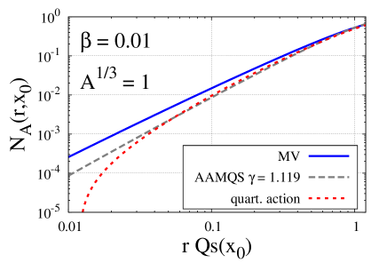
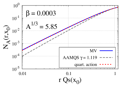
Figure 1: Left: scattering amplitude for an adjoint dipole
(N A = 2 N − N 2 subscript 𝑁 𝐴 2 𝑁 superscript 𝑁 2 N_{A}=2N-N^{2} Q s 2 = 0.168 superscript subscript 𝑄 𝑠 2 0.168 Q_{s}^{2}=0.168 2 and
Λ 2 = 0.0576 superscript Λ 2 0.0576 \Lambda^{2}=0.0576 2 .
Right: same for a nucleus with A = 200 𝐴 200 A=200 Q s 2 ∼ A 1 / 3 similar-to superscript subscript 𝑄 𝑠 2 superscript 𝐴 1 3 Q_{s}^{2}\sim A^{1/3} β A ∼ A − 2 / 3 similar-to subscript 𝛽 𝐴 superscript 𝐴 2 3 \beta_{A}\sim A^{-2/3}
One observes that the dipole scattering amplitude derived from the
quartic action is similar to the AAMQS model over a broad range,
r Q S ∼ > 0.04 superscript similar-to 𝑟 subscript 𝑄 𝑆 0.04 rQ_{S}\,\,\vbox{\hbox{$\buildrel\displaystyle>\over{\sim}$}}\,\,0.04 β 𝛽 \beta log 1 / r Λ ≫ 1 much-greater-than 1 𝑟 Λ 1 \log 1/r\Lambda\gg 1
On the right, we plot the scattering amplitude for a nucleus with
A = 200 𝐴 200 A=200 Q s 2 ∼ A 1 / 3 similar-to superscript subscript 𝑄 𝑠 2 superscript 𝐴 1 3 Q_{s}^{2}\sim A^{1/3} β A ∼ A − 2 / 3 similar-to subscript 𝛽 𝐴 superscript 𝐴 2 3 \beta_{A}\sim A^{-2/3} A 1 / 3 superscript 𝐴 1 3 A^{1/3} ρ 4 superscript 𝜌 4 \rho^{4} β A ∼ A − 2 / 3 similar-to subscript 𝛽 𝐴 superscript 𝐴 2 3 \beta_{A}\sim A^{-2/3} R p A subscript 𝑅 𝑝 𝐴 R_{pA}
Acknowledgements.
A.D. thanks M. Gyulassy for lively and useful discussions during a
seminar at Columbia University. The diagrams shown in the appendix
have been drawn with JaxoDraw
jaxo (
http://jaxodraw.sourceforge.net/).
We gratefully acknowledge support by the DOE Office of Nuclear Physics
through Grant No. DE-FG02-09ER41620, from the “Lab Directed Research
and Development” grant LDRD 10-043 (Brookhaven National Laboratory),
and for PSC-CUNY award 63382-0042, jointly funded by The Professional
Staff Congress and The City University of New York.
I Appendix
Expectation values of operators O [ ρ ] 𝑂 delimited-[] 𝜌 O[\rho]
⟨ O [ ρ ] ⟩ ≡ ∫ 𝒟 ρ O [ ρ ] e − S [ ρ ] / ∫ 𝒟 ρ e − S [ ρ ] . delimited-⟨⟩ 𝑂 delimited-[] 𝜌 𝒟 𝜌 𝑂 delimited-[] 𝜌 superscript 𝑒 𝑆 delimited-[] 𝜌 𝒟 𝜌 superscript 𝑒 𝑆 delimited-[] 𝜌 \langle O[\rho]\rangle\equiv\int{\cal D}\rho\;O[\rho]\;e^{-S[\rho]}~{}\Big{/}~{}\int{\cal D}\rho\;e^{-S[\rho]}~{}.
We work perturbatively in 1/κ 4 subscript 𝜅 4 \kappa_{4}
⟨ O [ ρ ] ⟩ delimited-⟨⟩ 𝑂 delimited-[] 𝜌 \displaystyle\langle O[\rho]\rangle ≡ \displaystyle\equiv ∫ 𝒟 ρ O [ ρ ] e − S G [ ρ ] [ 1 − 1 κ 4 ∫ d 2 𝕧 ⟂ ∫ 𝑑 v 1 − 𝑑 v 2 − ρ v 1 a ρ v 1 a ρ v 2 b ρ v 2 b ] ∫ 𝒟 ρ e − S G [ ρ ] [ 1 − 1 κ 4 ∫ d 2 𝕧 ⟂ ∫ 𝑑 v 1 − 𝑑 v 2 − ρ v 1 a ρ v 1 a ρ v 2 b ρ v 2 b ] 𝒟 𝜌 𝑂 delimited-[] 𝜌 superscript 𝑒 subscript 𝑆 𝐺 delimited-[] 𝜌 delimited-[] 1 1 subscript 𝜅 4 superscript 𝑑 2 subscript 𝕧 perpendicular-to differential-d superscript subscript 𝑣 1 differential-d superscript subscript 𝑣 2 subscript superscript 𝜌 𝑎 subscript 𝑣 1 subscript superscript 𝜌 𝑎 subscript 𝑣 1 subscript superscript 𝜌 𝑏 subscript 𝑣 2 subscript superscript 𝜌 𝑏 subscript 𝑣 2 𝒟 𝜌 superscript 𝑒 subscript 𝑆 𝐺 delimited-[] 𝜌 delimited-[] 1 1 subscript 𝜅 4 superscript 𝑑 2 subscript 𝕧 perpendicular-to differential-d superscript subscript 𝑣 1 differential-d superscript subscript 𝑣 2 subscript superscript 𝜌 𝑎 subscript 𝑣 1 subscript superscript 𝜌 𝑎 subscript 𝑣 1 subscript superscript 𝜌 𝑏 subscript 𝑣 2 subscript superscript 𝜌 𝑏 subscript 𝑣 2 \displaystyle\frac{\int\mathcal{D}\rho~{}O[\rho]~{}e^{-S_{G}[\rho]}\left[1-\frac{1}{\kappa_{4}}\int d^{2}\mathbb{v}_{\perp}\int dv_{1}^{-}dv_{2}^{-}\rho^{a}_{v_{1}}\rho^{a}_{v_{1}}\rho^{b}_{v_{2}}\rho^{b}_{v_{2}}\right]}{\int\mathcal{D}\rho~{}e^{-S_{G}[\rho]}\left[1-\frac{1}{\kappa_{4}}\int d^{2}\mathbb{v}_{\perp}\int dv_{1}^{-}dv_{2}^{-}\rho^{a}_{v_{1}}\rho^{a}_{v_{1}}\rho^{b}_{v_{2}}\rho^{b}_{v_{2}}\right]} (12)
= \displaystyle= ⟨ O [ ρ ] ( 1 − 1 κ 4 ∫ d 2 𝕧 ⟂ ∫ 𝑑 v 1 − 𝑑 v 2 − ρ v 1 a ρ v 1 a ρ v 2 b ρ v 2 b ) ⟩ G ⟨ 1 − 1 κ 4 ∫ d 2 𝕧 ⟂ ∫ 𝑑 v 1 − 𝑑 v 2 − ρ v 1 a ρ v 1 a ρ v 2 b ρ v 2 b ⟩ G . subscript delimited-⟨⟩ 𝑂 delimited-[] 𝜌 1 1 subscript 𝜅 4 superscript 𝑑 2 subscript 𝕧 perpendicular-to differential-d superscript subscript 𝑣 1 differential-d superscript subscript 𝑣 2 subscript superscript 𝜌 𝑎 subscript 𝑣 1 subscript superscript 𝜌 𝑎 subscript 𝑣 1 subscript superscript 𝜌 𝑏 subscript 𝑣 2 subscript superscript 𝜌 𝑏 subscript 𝑣 2 𝐺 subscript delimited-⟨⟩ 1 1 subscript 𝜅 4 superscript 𝑑 2 subscript 𝕧 perpendicular-to differential-d superscript subscript 𝑣 1 differential-d superscript subscript 𝑣 2 subscript superscript 𝜌 𝑎 subscript 𝑣 1 subscript superscript 𝜌 𝑎 subscript 𝑣 1 subscript superscript 𝜌 𝑏 subscript 𝑣 2 subscript superscript 𝜌 𝑏 subscript 𝑣 2 𝐺 \displaystyle\frac{\left<O[\rho]\left(1-\frac{1}{\kappa_{4}}\int d^{2}\mathbb{v}_{\perp}\int dv_{1}^{-}dv_{2}^{-}\rho^{a}_{v_{1}}\rho^{a}_{v_{1}}\rho^{b}_{v_{2}}\rho^{b}_{v_{2}}\right)\right>_{G}}{\langle 1-\frac{1}{\kappa_{4}}\int d^{2}\mathbb{v}_{\perp}\int dv_{1}^{-}dv_{2}^{-}\rho^{a}_{v_{1}}\rho^{a}_{v_{1}}\rho^{b}_{v_{2}}\rho^{b}_{v_{2}}\rangle_{G}}~{}~{}~{}.
In lattice regularization the denominator evaluates to
⟨ 1 − 1 κ 4 ∫ d 2 𝕧 ⟂ ∫ 𝑑 v 1 − 𝑑 v 2 − ρ v 1 a ρ v 1 a ρ v 2 b ρ v 2 b ⟩ G subscript delimited-⟨⟩ 1 1 subscript 𝜅 4 superscript 𝑑 2 subscript 𝕧 perpendicular-to differential-d superscript subscript 𝑣 1 differential-d superscript subscript 𝑣 2 subscript superscript 𝜌 𝑎 subscript 𝑣 1 subscript superscript 𝜌 𝑎 subscript 𝑣 1 subscript superscript 𝜌 𝑏 subscript 𝑣 2 subscript superscript 𝜌 𝑏 subscript 𝑣 2 𝐺 \displaystyle\left<1-\frac{1}{\kappa_{4}}\int d^{2}\mathbb{v}_{\perp}\int dv_{1}^{-}dv_{2}^{-}\rho^{a}_{v_{1}}\rho^{a}_{v_{1}}\rho^{b}_{v_{2}}\rho^{b}_{v_{2}}\right>_{G} (13)
= \displaystyle= 1 − 1 κ 4 N s Δ 𝕧 ⟂ { ( N c 2 − 1 ) 2 [ ∫ − ∞ ∞ 𝑑 v − μ 2 ( v − ) ] 2 + 2 ( N c 2 − 1 ) ∫ − ∞ ∞ 𝑑 v − μ 4 ( v − ) } , 1 1 subscript 𝜅 4 subscript 𝑁 𝑠 Δ subscript 𝕧 perpendicular-to superscript superscript subscript 𝑁 𝑐 2 1 2 superscript delimited-[] subscript superscript differential-d superscript 𝑣 superscript 𝜇 2 superscript 𝑣 2 2 superscript subscript 𝑁 𝑐 2 1 subscript superscript differential-d superscript 𝑣 superscript 𝜇 4 superscript 𝑣 \displaystyle 1-\frac{1}{\kappa_{4}}\frac{N_{s}}{\Delta\mathbb{v}_{\perp}}\left\{(N_{c}^{2}-1)^{2}\left[\int^{\infty}_{-\infty}dv^{-}\mu^{2}(v^{-})\right]^{2}+2~{}(N_{c}^{2}-1)\int^{\infty}_{-\infty}dv^{-}\mu^{4}(v^{-})\right\}~{}~{}~{},
where N s subscript 𝑁 𝑠 N_{s} Δ x ⟂ Δ subscript 𝑥 perpendicular-to \Delta x_{\perp} ⟨ ρ ρ ⟩ delimited-⟨⟩ 𝜌 𝜌 \langle\rho\rho\rangle
⟨ ρ a ( x − , 𝕩 ⟂ ) ρ b ( y − , 𝕪 ⟂ ) ⟩ = δ a b μ 2 ( x − ) δ ( x − − y − ) δ ( 𝕩 ⟂ − 𝕪 ⟂ ) . delimited-⟨⟩ superscript 𝜌 𝑎 superscript 𝑥 subscript 𝕩 perpendicular-to superscript 𝜌 𝑏 superscript 𝑦 subscript 𝕪 perpendicular-to superscript 𝛿 𝑎 𝑏 superscript 𝜇 2 superscript 𝑥 𝛿 superscript 𝑥 superscript 𝑦 𝛿 subscript 𝕩 perpendicular-to subscript 𝕪 perpendicular-to \langle\rho^{a}(x^{-},\mathbb{x}_{\perp})\,\rho^{b}(y^{-},\mathbb{y}_{\perp})\rangle=\delta^{ab}\mu^{2}(x^{-})\delta(x^{-}-y^{-})\delta(\mathbb{x}_{\perp}-\mathbb{y}_{\perp})~{}. (14)
I.1 Dipole Operator
We are interested in the expectation value of the dipole operator
defined as
D ^ ( 𝕩 ⟂ , y ⟂ ) ≡ 1 N c tr V ( 𝕩 ⟂ ) V † ( 𝕪 ⟂ ) . ^ 𝐷 subscript 𝕩 perpendicular-to subscript 𝑦 perpendicular-to 1 subscript 𝑁 𝑐 tr 𝑉 subscript 𝕩 perpendicular-to superscript 𝑉 † subscript 𝕪 perpendicular-to \hat{D}(\mathbb{x}_{\perp},y_{\perp})\equiv\frac{1}{N_{c}}{\rm tr}~{}V(\mathbb{x}_{\perp})V^{\dagger}(\mathbb{y}_{\perp})~{}~{}~{}. (15)
Here, V 𝑉 V
V ( 𝕩 ⟂ ) = 𝒫 exp { − i g 2 ∫ − ∞ ∞ 𝑑 z − 1 ∇ ⟂ 2 ρ a ( z − , 𝕩 ⟂ ) t a } , 𝑉 subscript 𝕩 perpendicular-to 𝒫 𝑖 superscript 𝑔 2 superscript subscript differential-d superscript 𝑧 1 subscript superscript ∇ 2 perpendicular-to subscript 𝜌 𝑎 superscript 𝑧 subscript 𝕩 perpendicular-to superscript 𝑡 𝑎 V(\mathbb{x}_{\perp})=\mathcal{P}\exp\left\{-ig^{2}\int_{-\infty}^{\infty}dz^{-}\frac{1}{\nabla^{2}_{\perp}}\rho_{a}(z^{-},\mathbb{x}_{\perp})t^{a}\right\}~{}~{}~{}, (16)
where
1 ∇ ⟂ 2 ρ a ( z − , 𝕩 ⟂ ) = ∫ d 2 𝕫 ⟂ G 0 ( 𝕩 ⟂ − 𝕫 ⟂ ) ρ a ( z − , 𝕫 ⟂ ) = − 1 g A + , 1 subscript superscript ∇ 2 perpendicular-to subscript 𝜌 𝑎 superscript 𝑧 subscript 𝕩 perpendicular-to superscript 𝑑 2 subscript 𝕫 perpendicular-to subscript 𝐺 0 subscript 𝕩 perpendicular-to subscript 𝕫 perpendicular-to subscript 𝜌 𝑎 superscript 𝑧 subscript 𝕫 perpendicular-to 1 𝑔 superscript 𝐴 \frac{1}{\nabla^{2}_{\perp}}\rho_{a}(z^{-},\mathbb{x}_{\perp})=\int d^{2}\mathbb{z}_{\perp}G_{0}(\mathbb{x}_{\perp}-\mathbb{z}_{\perp})\rho_{a}(z^{-},\mathbb{z}_{\perp})=-\frac{1}{g}A^{+}~{}~{}~{}, (17)
is proportional to the gauge potential in covariant gauge. The
matrices t a superscript 𝑡 𝑎 t^{a} tr t a t b = 1 2 δ a b tr superscript 𝑡 𝑎 superscript 𝑡 𝑏 1 2 superscript 𝛿 𝑎 𝑏 {\rm tr}~{}t^{a}t^{b}=\frac{1}{2}\delta^{ab}
G 0 subscript 𝐺 0 G_{0}
∂ 2 ∂ 𝕫 ⟂ 2 G 0 ( 𝕩 ⟂ − 𝕫 ⟂ ) = δ ( 𝕩 ⟂ − 𝕫 ⟂ ) ; superscript 2 subscript superscript 𝕫 2 perpendicular-to subscript 𝐺 0 subscript 𝕩 perpendicular-to subscript 𝕫 perpendicular-to 𝛿 subscript 𝕩 perpendicular-to subscript 𝕫 perpendicular-to \frac{\partial^{2}}{\partial\mathbb{z}^{2}_{\perp}}G_{0}(\mathbb{x}_{\perp}-\mathbb{z}_{\perp})=\delta(\mathbb{x}_{\perp}-\mathbb{z}_{\perp})~{}~{}~{}; (18)
G 0 ( 𝕩 ⟂ − 𝕫 ⟂ ) = − ∫ d 2 𝕜 ⟂ ( 2 π ) 2 e i 𝕜 ⟂ ⋅ ( 𝕩 ⟂ − 𝕫 ⟂ ) 𝕜 ⟂ 2 . subscript 𝐺 0 subscript 𝕩 perpendicular-to subscript 𝕫 perpendicular-to superscript 𝑑 2 subscript 𝕜 perpendicular-to superscript 2 𝜋 2 superscript 𝑒 ⋅ 𝑖 subscript 𝕜 perpendicular-to subscript 𝕩 perpendicular-to subscript 𝕫 perpendicular-to subscript superscript 𝕜 2 perpendicular-to G_{0}(\mathbb{x}_{\perp}-\mathbb{z}_{\perp})=-\int\frac{d^{2}\mathbb{k}_{\perp}}{(2\pi)^{2}}\frac{e^{i\mathbb{k}_{\perp}\cdot(\mathbb{x}_{\perp}-\mathbb{z}_{\perp})}}{\mathbb{k}^{2}_{\perp}}~{}~{}~{}. (19)
With this propagator we can write the Wilson line as
V ( 𝕩 ⟂ ) = 𝒫 exp { − i g 2 ∫ − ∞ ∞ 𝑑 z − ∫ d 2 𝕫 ⟂ G 0 ( 𝕩 ⟂ − 𝕫 ⟂ ) ρ a ( z − , 𝕫 ⟂ ) t a } . 𝑉 subscript 𝕩 perpendicular-to 𝒫 𝑖 superscript 𝑔 2 subscript superscript differential-d superscript 𝑧 superscript 𝑑 2 subscript 𝕫 perpendicular-to subscript 𝐺 0 subscript 𝕩 perpendicular-to subscript 𝕫 perpendicular-to subscript 𝜌 𝑎 superscript 𝑧 subscript 𝕫 perpendicular-to superscript 𝑡 𝑎 V(\mathbb{x}_{\perp})=\mathcal{P}\exp\left\{-ig^{2}\int^{\infty}_{-\infty}dz^{-}\int d^{2}\mathbb{z}_{\perp}\,G_{0}(\mathbb{x}_{\perp}-\mathbb{z}_{\perp})\,\rho_{a}(z^{-},\mathbb{z}_{\perp})\,t^{a}\right\}~{}~{}~{}. (20)
The correlator ⟨ V ( 𝕩 ⟂ ) V † ( 𝕪 ⟂ ) ⟩ delimited-⟨⟩ 𝑉 subscript 𝕩 perpendicular-to superscript 𝑉 † subscript 𝕪 perpendicular-to \langle V(\mathbb{x}_{\perp})V^{\dagger}(\mathbb{y}_{\perp})\rangle GelisPeshier
⟨ V ( 𝕩 ⟂ ) V † ( 𝕪 ⟂ ) ⟩ G = exp { − g 4 2 ( t a t a ) [ ∫ − ∞ ∞ 𝑑 z − μ 2 ( z − ) ] ∫ d 2 𝕫 ⟂ [ G 0 ( 𝕩 ⟂ − 𝕫 ⟂ ) − G 0 ( 𝕪 ⟂ − 𝕫 ⟂ ) ] 2 } . subscript delimited-⟨⟩ 𝑉 subscript 𝕩 perpendicular-to superscript 𝑉 † subscript 𝕪 perpendicular-to 𝐺 superscript 𝑔 4 2 superscript 𝑡 𝑎 subscript 𝑡 𝑎 delimited-[] superscript subscript differential-d superscript 𝑧 superscript 𝜇 2 superscript 𝑧 superscript 𝑑 2 subscript 𝕫 perpendicular-to superscript delimited-[] subscript 𝐺 0 subscript 𝕩 perpendicular-to subscript 𝕫 perpendicular-to subscript 𝐺 0 subscript 𝕪 perpendicular-to subscript 𝕫 perpendicular-to 2 \langle V(\mathbb{x}_{\perp})V^{\dagger}(\mathbb{y}_{\perp})\rangle_{G}=\exp\left\{-\frac{g^{4}}{2}(t^{a}t_{a})\left[\int_{-\infty}^{\infty}dz^{-}\mu^{2}(z^{-})\right]\int d^{2}\mathbb{z}_{\perp}\left[G_{0}(\mathbb{x}_{\perp}-\mathbb{z}_{\perp})-G_{0}(\mathbb{y}_{\perp}-\mathbb{z}_{\perp})\right]^{2}\right\}~{}~{}. (21)
Note that this is diagonal in color (proportional to 1 1 3 × 3 1 subscript 1 3 3 1\!\!1_{3\times 3} g 2 superscript 𝑔 2 g^{2}
V ( 𝕩 ⟂ ) 𝑉 subscript 𝕩 perpendicular-to \displaystyle V(\mathbb{x}_{\perp}) = \displaystyle= 1 − i g 2 ∫ d 2 𝕫 ⟂ 1 G 0 ( 𝕩 ⟂ − 𝕫 ⟂ 1 ) ∫ − ∞ ∞ 𝑑 z 1 − ρ a ( z 1 ) t a 1 𝑖 superscript 𝑔 2 superscript 𝑑 2 subscript 𝕫 perpendicular-to absent 1 subscript 𝐺 0 subscript 𝕩 perpendicular-to subscript 𝕫 perpendicular-to absent 1 subscript superscript differential-d superscript subscript 𝑧 1 superscript 𝜌 𝑎 subscript 𝑧 1 superscript 𝑡 𝑎 \displaystyle 1-ig^{2}\int d^{2}\mathbb{z}_{\perp 1}G_{0}(\mathbb{x}_{\perp}-\mathbb{z}_{\perp 1})\int^{\infty}_{-\infty}dz_{1}^{-}\rho^{a}(z_{1})t^{a} (22)
− g 4 ∫ d 2 𝕫 ⟂ 1 d 2 𝕫 ⟂ 2 G 0 ( 𝕩 ⟂ − 𝕫 ⟂ 1 ) G 0 ( 𝕩 ⟂ − 𝕫 ⟂ 2 ) ∫ − ∞ ∞ 𝑑 z 1 − ∫ z 1 − ∞ 𝑑 z 2 − ρ a ( z 1 ) ρ b ( z 2 ) t a t b superscript 𝑔 4 superscript 𝑑 2 subscript 𝕫 perpendicular-to absent 1 superscript 𝑑 2 subscript 𝕫 perpendicular-to absent 2 subscript 𝐺 0 subscript 𝕩 perpendicular-to subscript 𝕫 perpendicular-to absent 1 subscript 𝐺 0 subscript 𝕩 perpendicular-to subscript 𝕫 perpendicular-to absent 2 subscript superscript differential-d superscript subscript 𝑧 1 subscript superscript superscript subscript 𝑧 1 differential-d superscript subscript 𝑧 2 superscript 𝜌 𝑎 subscript 𝑧 1 superscript 𝜌 𝑏 subscript 𝑧 2 superscript 𝑡 𝑎 superscript 𝑡 𝑏 \displaystyle-g^{4}\int d^{2}\mathbb{z}_{\perp 1}d^{2}\mathbb{z}_{\perp 2}G_{0}(\mathbb{x}_{\perp}-\mathbb{z}_{\perp 1})G_{0}(\mathbb{x}_{\perp}-\mathbb{z}_{\perp 2})\int^{\infty}_{-\infty}dz_{1}^{-}\int^{\infty}_{z_{1}^{-}}dz_{2}^{-}\rho^{a}(z_{1})\rho^{b}(z_{2})t^{a}t^{b}
+ ⋯ ⋯ \displaystyle+\cdots
V † ( 𝕪 ⟂ ) superscript 𝑉 † subscript 𝕪 perpendicular-to \displaystyle V^{\dagger}(\mathbb{y}_{\perp}) = \displaystyle= 1 + i g 2 ∫ d 2 𝕦 ⟂ 1 G 0 ( 𝕪 ⟂ − 𝕦 ⟂ 1 ) ∫ − ∞ ∞ 𝑑 u 1 − ρ a ( u 1 ) t a 1 𝑖 superscript 𝑔 2 superscript 𝑑 2 subscript 𝕦 perpendicular-to absent 1 subscript 𝐺 0 subscript 𝕪 perpendicular-to subscript 𝕦 perpendicular-to absent 1 subscript superscript differential-d superscript subscript 𝑢 1 superscript 𝜌 𝑎 subscript 𝑢 1 superscript 𝑡 𝑎 \displaystyle 1+ig^{2}\int d^{2}\mathbb{u}_{\perp 1}G_{0}(\mathbb{y}_{\perp}-\mathbb{u}_{\perp 1})\int^{\infty}_{-\infty}du_{1}^{-}\rho^{a}(u_{1})t^{a} (23)
− g 4 ∫ d 2 𝕦 ⟂ 1 d 2 𝕦 ⟂ 2 G 0 ( 𝕪 ⟂ − 𝕦 ⟂ 1 ) G 0 ( 𝕪 ⟂ − 𝕦 ⟂ 2 ) ∫ − ∞ ∞ 𝑑 u 1 − ∫ − ∞ u 1 − 𝑑 u 2 − ρ a ( u 1 ) ρ b ( u 2 ) t a t b superscript 𝑔 4 superscript 𝑑 2 subscript 𝕦 perpendicular-to absent 1 superscript 𝑑 2 subscript 𝕦 perpendicular-to absent 2 subscript 𝐺 0 subscript 𝕪 perpendicular-to subscript 𝕦 perpendicular-to absent 1 subscript 𝐺 0 subscript 𝕪 perpendicular-to subscript 𝕦 perpendicular-to absent 2 subscript superscript differential-d superscript subscript 𝑢 1 subscript superscript superscript subscript 𝑢 1 differential-d superscript subscript 𝑢 2 superscript 𝜌 𝑎 subscript 𝑢 1 superscript 𝜌 𝑏 subscript 𝑢 2 superscript 𝑡 𝑎 superscript 𝑡 𝑏 \displaystyle-g^{4}\int d^{2}\mathbb{u}_{\perp 1}d^{2}\mathbb{u}_{\perp 2}G_{0}(\mathbb{y}_{\perp}-\mathbb{u}_{\perp 1})G_{0}(\mathbb{y}_{\perp}-\mathbb{u}_{\perp 2})\int^{\infty}_{-\infty}du_{1}^{-}\int^{u_{1}^{-}}_{-\infty}du_{2}^{-}\rho^{a}(u_{1})\rho^{b}(u_{2})t^{a}t^{b}
+ ⋯ ⋯ \displaystyle+\cdots
For brevity we only write the terms up to 𝒪 ( g 4 ) 𝒪 superscript 𝑔 4 \mathcal{O}(g^{4}) 𝒪 ( g 8 ) 𝒪 superscript 𝑔 8 \mathcal{O}(g^{8})
To zeroth order in g 𝑔 g
𝒪 ( g 0 ) = 1 . 𝒪 superscript 𝑔 0 1 \mathcal{O}\left(g^{0}\right)=1~{}~{}~{}.
The order g 2 superscript 𝑔 2 g^{2} ⟨ ρ a ( z ) ⟩ = 0 delimited-⟨⟩ superscript 𝜌 𝑎 𝑧 0 \langle\rho^{a}(z)\rangle=0
𝒪 ( g 2 ) = 0 . 𝒪 superscript 𝑔 2 0 \mathcal{O}\left(g^{2}\right)=0~{}~{}~{}.
I.2 Order g 4 superscript 𝑔 4 g^{4}
The first non-trivial contribution arises at 𝒪 ( g 4 ) 𝒪 superscript 𝑔 4 \mathcal{O}(g^{4})
− g 4 ∫ d 2 𝕫 ⟂ 1 d 2 𝕫 ⟂ 2 G 0 ( 𝕩 ⟂ − 𝕫 ⟂ 1 ) G 0 ( 𝕩 ⟂ − 𝕫 ⟂ 2 ) ∫ − ∞ ∞ 𝑑 z 1 − ∫ z 1 − ∞ 𝑑 z 2 − ⟨ ρ a ( z 1 ) ρ b ( z 2 ) ⟩ t a t b , superscript 𝑔 4 superscript 𝑑 2 subscript 𝕫 perpendicular-to absent 1 superscript 𝑑 2 subscript 𝕫 perpendicular-to absent 2 subscript 𝐺 0 subscript 𝕩 perpendicular-to subscript 𝕫 perpendicular-to absent 1 subscript 𝐺 0 subscript 𝕩 perpendicular-to subscript 𝕫 perpendicular-to absent 2 subscript superscript differential-d superscript subscript 𝑧 1 subscript superscript superscript subscript 𝑧 1 differential-d superscript subscript 𝑧 2 delimited-⟨⟩ superscript 𝜌 𝑎 subscript 𝑧 1 superscript 𝜌 𝑏 subscript 𝑧 2 superscript 𝑡 𝑎 superscript 𝑡 𝑏 -g^{4}\int d^{2}\mathbb{z}_{\perp 1}d^{2}\mathbb{z}_{\perp 2}G_{0}(\mathbb{x}_{\perp}-\mathbb{z}_{\perp 1})G_{0}(\mathbb{x}_{\perp}-\mathbb{z}_{\perp 2})\int^{\infty}_{-\infty}dz_{1}^{-}\int^{\infty}_{z_{1}^{-}}dz_{2}^{-}\langle\rho^{a}(z_{1})\rho^{b}(z_{2})\rangle t^{a}t^{b}~{}~{}, (24)
− g 4 ∫ d 2 𝕦 ⟂ 1 d 2 𝕦 ⟂ 2 G 0 ( 𝕪 ⟂ − 𝕦 ⟂ 1 ) G 0 ( 𝕪 ⟂ − 𝕦 ⟂ 2 ) ∫ − ∞ ∞ 𝑑 u 1 − ∫ − ∞ u 1 − 𝑑 u 2 − ⟨ ρ a ( u 1 ) ρ b ( u 2 ) ⟩ t a t b , superscript 𝑔 4 superscript 𝑑 2 subscript 𝕦 perpendicular-to absent 1 superscript 𝑑 2 subscript 𝕦 perpendicular-to absent 2 subscript 𝐺 0 subscript 𝕪 perpendicular-to subscript 𝕦 perpendicular-to absent 1 subscript 𝐺 0 subscript 𝕪 perpendicular-to subscript 𝕦 perpendicular-to absent 2 subscript superscript differential-d superscript subscript 𝑢 1 subscript superscript superscript subscript 𝑢 1 differential-d superscript subscript 𝑢 2 delimited-⟨⟩ superscript 𝜌 𝑎 subscript 𝑢 1 superscript 𝜌 𝑏 subscript 𝑢 2 superscript 𝑡 𝑎 superscript 𝑡 𝑏 -g^{4}\int d^{2}\mathbb{u}_{\perp 1}d^{2}\mathbb{u}_{\perp 2}G_{0}(\mathbb{y}_{\perp}-\mathbb{u}_{\perp 1})G_{0}(\mathbb{y}_{\perp}-\mathbb{u}_{\perp 2})\int^{\infty}_{-\infty}du_{1}^{-}\int^{u_{1}^{-}}_{-\infty}du_{2}^{-}\langle\rho^{a}(u_{1})\rho^{b}(u_{2})\rangle t^{a}t^{b}~{}~{}, (25)
g 4 ∫ d 2 𝕫 ⟂ 1 ∫ d 2 𝕦 ⟂ 1 G 0 ( 𝕩 ⟂ − 𝕫 ⟂ 1 ) G 0 ( 𝕪 ⟂ − 𝕦 ⟂ 1 ) ∫ − ∞ ∞ 𝑑 z 1 − ∫ − ∞ ∞ 𝑑 u 1 − ⟨ ρ a ( z 1 ) ρ b ( u 1 ) ⟩ t a t b . superscript 𝑔 4 superscript 𝑑 2 subscript 𝕫 perpendicular-to absent 1 superscript 𝑑 2 subscript 𝕦 perpendicular-to absent 1 subscript 𝐺 0 subscript 𝕩 perpendicular-to subscript 𝕫 perpendicular-to absent 1 subscript 𝐺 0 subscript 𝕪 perpendicular-to subscript 𝕦 perpendicular-to absent 1 subscript superscript differential-d superscript subscript 𝑧 1 subscript superscript differential-d superscript subscript 𝑢 1 delimited-⟨⟩ superscript 𝜌 𝑎 subscript 𝑧 1 superscript 𝜌 𝑏 subscript 𝑢 1 superscript 𝑡 𝑎 superscript 𝑡 𝑏 g^{4}\int d^{2}\mathbb{z}_{\perp 1}\int d^{2}\mathbb{u}_{\perp 1}G_{0}(\mathbb{x}_{\perp}-\mathbb{z}_{\perp 1})G_{0}(\mathbb{y}_{\perp}-\mathbb{u}_{\perp 1})\int^{\infty}_{-\infty}dz_{1}^{-}\int^{\infty}_{-\infty}du_{1}^{-}\langle\rho^{a}(z_{1})\rho^{b}(u_{1})\rangle t^{a}t^{b}~{}~{}. (26)
Using (12 21
− \displaystyle- g 4 2 t a t a ∫ − ∞ ∞ 𝑑 z − μ 2 ( z − ) ∫ d 2 𝕫 ⟂ G 0 2 ( 𝕩 ⟂ − 𝕫 ⟂ ) superscript 𝑔 4 2 superscript 𝑡 𝑎 subscript 𝑡 𝑎 superscript subscript differential-d superscript 𝑧 superscript 𝜇 2 superscript 𝑧 superscript 𝑑 2 subscript 𝕫 perpendicular-to superscript subscript 𝐺 0 2 subscript 𝕩 perpendicular-to subscript 𝕫 perpendicular-to \displaystyle\frac{g^{4}}{2}t^{a}t_{a}\int_{-\infty}^{\infty}dz^{-}\mu^{2}(z^{-})\int d^{2}\mathbb{z}_{\perp}G_{0}^{2}(\mathbb{x}_{\perp}-\mathbb{z}_{\perp}) (27)
+ \displaystyle+ g 4 κ 4 ∫ d 2 𝕫 ⟂ 1 d 2 𝕫 ⟂ 2 d 2 𝕧 ⟂ G 0 ( 𝕩 ⟂ − 𝕫 ⟂ 1 ) G 0 ( 𝕩 ⟂ − 𝕫 ⟂ 2 ) superscript 𝑔 4 subscript 𝜅 4 superscript 𝑑 2 subscript 𝕫 perpendicular-to absent 1 superscript 𝑑 2 subscript 𝕫 perpendicular-to absent 2 superscript 𝑑 2 subscript 𝕧 perpendicular-to subscript 𝐺 0 subscript 𝕩 perpendicular-to subscript 𝕫 perpendicular-to absent 1 subscript 𝐺 0 subscript 𝕩 perpendicular-to subscript 𝕫 perpendicular-to absent 2 \displaystyle\frac{g^{4}}{\kappa_{4}}\int d^{2}\mathbb{z}_{\perp 1}d^{2}\mathbb{z}_{\perp 2}d^{2}\mathbb{v}_{\perp}G_{0}(\mathbb{x}_{\perp}-\mathbb{z}_{\perp 1})G_{0}(\mathbb{x}_{\perp}-\mathbb{z}_{\perp 2})
× ∫ − ∞ ∞ d z 1 − ∫ z 1 − ∞ d z 2 − ∫ d v 1 − d v 2 − ⟨ ρ z 1 a ρ z 2 b ρ v 1 c ρ v 1 c ρ v 2 d ρ v 2 d ⟩ t a t b . \displaystyle\times\int_{-\infty}^{\infty}dz_{1}^{-}\int_{z_{1}^{-}}^{\infty}dz_{2}^{-}\int dv_{1}^{-}dv_{2}^{-}\langle\rho_{z_{1}}^{a}\rho_{z_{2}}^{b}\rho_{v_{1}}^{c}\rho_{v_{1}}^{c}\rho_{v_{2}}^{d}\rho_{v_{2}}^{d}\rangle t^{a}t^{b}~{}.
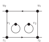
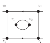
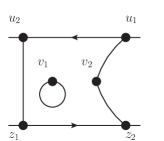
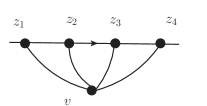
All possible contractions for the second term in the above expression are
⟨ ρ z 1 a ρ z 2 b ρ v 1 c ρ v 1 c ρ v 2 d ρ v 2 d ⟩ = ⟨ ρ z 1 a ρ z 2 b ⟩ [ ⟨ ρ v 1 c ρ v 1 c ⟩ ⟨ ρ v 2 d ρ v 2 d ⟩ + 2 ⟨ ρ v 1 c ρ v 2 d ⟩ ⟨ ρ v 1 c ρ v 2 d ⟩ ] delimited-⟨⟩ superscript subscript 𝜌 subscript 𝑧 1 𝑎 superscript subscript 𝜌 subscript 𝑧 2 𝑏 superscript subscript 𝜌 subscript 𝑣 1 𝑐 superscript subscript 𝜌 subscript 𝑣 1 𝑐 superscript subscript 𝜌 subscript 𝑣 2 𝑑 superscript subscript 𝜌 subscript 𝑣 2 𝑑 delimited-⟨⟩ superscript subscript 𝜌 subscript 𝑧 1 𝑎 superscript subscript 𝜌 subscript 𝑧 2 𝑏 delimited-[] delimited-⟨⟩ superscript subscript 𝜌 subscript 𝑣 1 𝑐 superscript subscript 𝜌 subscript 𝑣 1 𝑐 delimited-⟨⟩ superscript subscript 𝜌 subscript 𝑣 2 𝑑 superscript subscript 𝜌 subscript 𝑣 2 𝑑 2 delimited-⟨⟩ superscript subscript 𝜌 subscript 𝑣 1 𝑐 superscript subscript 𝜌 subscript 𝑣 2 𝑑 delimited-⟨⟩ superscript subscript 𝜌 subscript 𝑣 1 𝑐 superscript subscript 𝜌 subscript 𝑣 2 𝑑 \displaystyle\langle\rho_{z_{1}}^{a}\rho_{z_{2}}^{b}\rho_{v_{1}}^{c}\rho_{v_{1}}^{c}\rho_{v_{2}}^{d}\rho_{v_{2}}^{d}\rangle=\langle\rho_{z_{1}}^{a}\rho_{z_{2}}^{b}\rangle\left[\langle\rho_{v_{1}}^{c}\rho_{v_{1}}^{c}\rangle\langle\rho_{v_{2}}^{d}\rho_{v_{2}}^{d}\rangle+2~{}\langle\rho_{v_{1}}^{c}\rho_{v_{2}}^{d}\rangle\langle\rho_{v_{1}}^{c}\rho_{v_{2}}^{d}\rangle\right]
+ 4 ⟨ ρ z 1 a ρ v 1 c ⟩ [ ⟨ ρ z 2 b ρ v 1 c ⟩ ⟨ ρ v 2 d ρ v 2 d ⟩ + 2 ⟨ ρ z 2 b ρ v 2 d ⟩ ⟨ ρ v 1 c ρ v 2 d ⟩ ] , 4 delimited-⟨⟩ superscript subscript 𝜌 subscript 𝑧 1 𝑎 superscript subscript 𝜌 subscript 𝑣 1 𝑐 delimited-[] delimited-⟨⟩ superscript subscript 𝜌 subscript 𝑧 2 𝑏 superscript subscript 𝜌 subscript 𝑣 1 𝑐 delimited-⟨⟩ superscript subscript 𝜌 subscript 𝑣 2 𝑑 superscript subscript 𝜌 subscript 𝑣 2 𝑑 2 delimited-⟨⟩ superscript subscript 𝜌 subscript 𝑧 2 𝑏 superscript subscript 𝜌 subscript 𝑣 2 𝑑 delimited-⟨⟩ superscript subscript 𝜌 subscript 𝑣 1 𝑐 superscript subscript 𝜌 subscript 𝑣 2 𝑑 \displaystyle+4~{}\langle\rho_{z_{1}}^{a}\rho_{v_{1}}^{c}\rangle\left[\langle\rho_{z_{2}}^{b}\rho_{v_{1}}^{c}\rangle\langle\rho_{v_{2}}^{d}\rho_{v_{2}}^{d}\rangle+2~{}\langle\rho_{z_{2}}^{b}\rho_{v_{2}}^{d}\rangle\langle\rho_{v_{1}}^{c}\rho_{v_{2}}^{d}\rangle\right], (28)
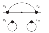
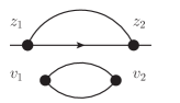
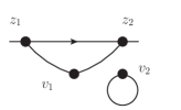
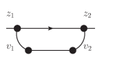
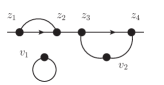
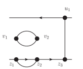
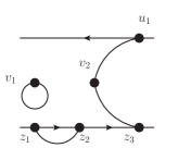
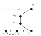
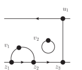
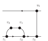
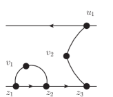
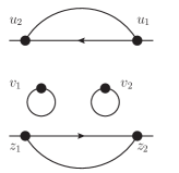
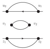
and are shown diagrammatically in fig. 2
Figure 2: ⟨ V ⟩ delimited-⟨⟩ 𝑉 \langle V\rangle g 4 / κ 4 superscript 𝑔 4 subscript 𝜅 4 g^{4}/\kappa_{4}
Using (14 13
1 1 − 1 κ 4 N s Δ 𝕧 ⟂ { ( N c 2 − 1 ) 2 [ ∫ − ∞ ∞ 𝑑 v − μ 2 ( v − ) ] 2 + 2 ( N c 2 − 1 ) ∫ − ∞ ∞ 𝑑 v − μ 4 ( v − ) } × \displaystyle\frac{1}{1-\frac{1}{\kappa_{4}}\frac{N_{s}}{\Delta\mathbb{v}_{\perp}}\left\{(N_{c}^{2}-1)^{2}\left[\int^{\infty}_{-\infty}dv^{-}\mu^{2}(v^{-})\right]^{2}+2~{}(N_{c}^{2}-1)\int^{\infty}_{-\infty}dv^{-}\mu^{4}(v^{-})\right\}}\times
{ − g 4 2 t a t a ∫ − ∞ ∞ d z − μ 2 ( z − ) ∫ d 2 𝕫 ⟂ G 0 2 ( 𝕩 ⟂ − 𝕫 ⟂ ) × \displaystyle\left\{-\frac{g^{4}}{2}t^{a}t_{a}\int_{-\infty}^{\infty}dz^{-}\mu^{2}(z^{-})\int d^{2}\mathbb{z}_{\perp}G_{0}^{2}(\mathbb{x}_{\perp}-\mathbb{z}_{\perp})\times\right.
{ 1 − 1 κ 4 N s Δ 𝕧 ⟂ [ ( N c 2 − 1 ) 2 [ ∫ − ∞ ∞ 𝑑 v − μ 2 ( v − ) ] 2 + 2 ( N c 2 − 1 ) ∫ − ∞ ∞ 𝑑 v − μ 4 ( v − ) ] } + limit-from 1 1 subscript 𝜅 4 subscript 𝑁 𝑠 Δ subscript 𝕧 perpendicular-to delimited-[] superscript superscript subscript 𝑁 𝑐 2 1 2 superscript delimited-[] subscript superscript differential-d superscript 𝑣 superscript 𝜇 2 superscript 𝑣 2 2 superscript subscript 𝑁 𝑐 2 1 subscript superscript differential-d superscript 𝑣 superscript 𝜇 4 superscript 𝑣 \displaystyle\left.\left\{1-\frac{1}{\kappa_{4}}\frac{N_{s}}{\Delta\mathbb{v}_{\perp}}\left[(N_{c}^{2}-1)^{2}\left[\int^{\infty}_{-\infty}dv^{-}\mu^{2}(v^{-})\right]^{2}+2~{}(N_{c}^{2}-1)\int^{\infty}_{-\infty}dv^{-}\mu^{4}(v^{-})\right]\right\}+\right.
2 g 4 κ 4 t a t a Δ 𝕧 ⟂ ∫ d 2 𝕫 ⟂ G 0 2 ( 𝕩 ⟂ − 𝕫 ⟂ ) [ ( N c 2 − 1 ) ∫ − ∞ ∞ d z − μ 2 ( z − ) ∫ − ∞ ∞ d v − μ 4 ( v − ) + 2 ∫ − ∞ ∞ d z − μ 6 ( z − ) ] } . \displaystyle\left.2\frac{g^{4}}{\kappa_{4}}\frac{t^{a}t_{a}}{\Delta\mathbb{v}_{\perp}}\int d^{2}\mathbb{z}_{\perp}G_{0}^{2}(\mathbb{x}_{\perp}-\mathbb{z}_{\perp})\left[(N_{c}^{2}-1)\int_{-\infty}^{\infty}dz^{-}\mu^{2}(z^{-})\int_{-\infty}^{\infty}dv^{-}\mu^{4}(v^{-})+2\int_{-\infty}^{\infty}dz^{-}\mu^{6}(z^{-})\right]\right\}~{}~{}. (29)
The third line in the above expression cancels the normalization
factor once the latter is expanded to leading order in 1 / κ 4 1 subscript 𝜅 4 1/\kappa_{4}
− \displaystyle- g 4 2 t a t a ∫ d 2 𝕫 ⟂ G 0 2 ( 𝕩 ⟂ − 𝕫 ⟂ ) superscript 𝑔 4 2 superscript 𝑡 𝑎 subscript 𝑡 𝑎 superscript 𝑑 2 subscript 𝕫 perpendicular-to superscript subscript 𝐺 0 2 subscript 𝕩 perpendicular-to subscript 𝕫 perpendicular-to \displaystyle\frac{g^{4}}{2}t^{a}t_{a}\int d^{2}\mathbb{z}_{\perp}G_{0}^{2}(\mathbb{x}_{\perp}-\mathbb{z}_{\perp}) (30)
× { ∫ − ∞ ∞ d z − μ 2 ( z − ) \displaystyle\times\left\{\int_{-\infty}^{\infty}dz^{-}\mu^{2}(z^{-})\right.
− 4 κ 4 Δ 𝕧 ⟂ [ ( N c 2 − 1 ) ∫ − ∞ ∞ d z − μ 2 ( z − ) ∫ − ∞ ∞ d v − μ 4 ( v − ) + 2 ∫ − ∞ ∞ d z − μ 6 ( z − ) ] } . \displaystyle\left.~{}~{}-\frac{4}{\kappa_{4}\Delta\mathbb{v}_{\perp}}\left[(N_{c}^{2}-1)\int_{-\infty}^{\infty}dz^{-}\mu^{2}(z^{-})\int_{-\infty}^{\infty}dv^{-}\mu^{4}(v^{-})+2\int_{-\infty}^{\infty}dz^{-}\mu^{6}(z^{-})\right]\right\}~{}.
The correction is absorbed into a renormalization of
∫ − ∞ ∞ 𝑑 z − μ 2 ( z − ) superscript subscript differential-d superscript 𝑧 superscript 𝜇 2 superscript 𝑧 \int_{-\infty}^{\infty}dz^{-}\mu^{2}(z^{-}) ⟨ ρ ρ ⟩ delimited-⟨⟩ 𝜌 𝜌 \langle\rho\rho\rangle
∫ − ∞ ∞ 𝑑 z − μ ~ 2 ( z − ) = superscript subscript differential-d superscript 𝑧 superscript ~ 𝜇 2 superscript 𝑧 absent \displaystyle\int_{-\infty}^{\infty}dz^{-}\tilde{\mu}^{2}(z^{-})=
∫ − ∞ ∞ 𝑑 z − μ 2 ( z − ) − 4 κ 4 Δ 𝕧 ⟂ [ ( N c 2 − 1 ) ∫ − ∞ ∞ 𝑑 z − μ 2 ( z − ) ∫ − ∞ ∞ 𝑑 v − μ 4 ( v − ) + 2 ∫ − ∞ ∞ 𝑑 z − μ 6 ( z − ) ] . superscript subscript differential-d superscript 𝑧 superscript 𝜇 2 superscript 𝑧 4 subscript 𝜅 4 Δ subscript 𝕧 perpendicular-to delimited-[] superscript subscript 𝑁 𝑐 2 1 superscript subscript differential-d superscript 𝑧 superscript 𝜇 2 superscript 𝑧 superscript subscript differential-d superscript 𝑣 superscript 𝜇 4 superscript 𝑣 2 superscript subscript differential-d superscript 𝑧 superscript 𝜇 6 superscript 𝑧 \displaystyle\int_{-\infty}^{\infty}dz^{-}\mu^{2}(z^{-})-\frac{4}{\kappa_{4}\Delta\mathbb{v}_{\perp}}\left[(N_{c}^{2}-1)\int_{-\infty}^{\infty}dz^{-}\mu^{2}(z^{-})\int_{-\infty}^{\infty}dv^{-}\mu^{4}(v^{-})+2\int_{-\infty}^{\infty}dz^{-}\mu^{6}(z^{-})\right]~{}. (31)
Finally, the expectation value of V ( x ⟂ ) 𝑉 subscript 𝑥 perpendicular-to V(x_{\perp}) g 4 superscript 𝑔 4 g^{4}
− g 4 2 t a t a ∫ − ∞ ∞ 𝑑 z − μ ~ 2 ( z − ) ∫ d 2 𝕫 ⟂ G 0 2 ( 𝕩 ⟂ − 𝕫 ⟂ ) . superscript 𝑔 4 2 superscript 𝑡 𝑎 subscript 𝑡 𝑎 superscript subscript differential-d superscript 𝑧 superscript ~ 𝜇 2 superscript 𝑧 superscript 𝑑 2 subscript 𝕫 perpendicular-to superscript subscript 𝐺 0 2 subscript 𝕩 perpendicular-to subscript 𝕫 perpendicular-to -\frac{g^{4}}{2}t^{a}t_{a}~{}\int_{-\infty}^{\infty}dz^{-}\tilde{\mu}^{2}(z^{-})\int d^{2}\mathbb{z}_{\perp}G_{0}^{2}(\mathbb{x}_{\perp}-\mathbb{z}_{\perp})~{}~{}. (32)
Similarly, ⟨ V † ( y ⟂ ) ⟩ delimited-⟨⟩ superscript 𝑉 † subscript 𝑦 perpendicular-to \langle V^{\dagger}(y_{\perp})\rangle
− g 4 2 t a t a ∫ − ∞ ∞ 𝑑 z − μ ~ 2 ( z − ) ∫ d 2 𝕦 ⟂ G 0 2 ( 𝕪 ⟂ − 𝕦 ⟂ ) . superscript 𝑔 4 2 superscript 𝑡 𝑎 subscript 𝑡 𝑎 superscript subscript differential-d superscript 𝑧 superscript ~ 𝜇 2 superscript 𝑧 superscript 𝑑 2 subscript 𝕦 perpendicular-to superscript subscript 𝐺 0 2 subscript 𝕪 perpendicular-to subscript 𝕦 perpendicular-to -\frac{g^{4}}{2}t^{a}t_{a}~{}\int_{-\infty}^{\infty}dz^{-}\tilde{\mu}^{2}(z^{-})\int d^{2}\mathbb{u}_{\perp}G_{0}^{2}(\mathbb{y}_{\perp}-\mathbb{u}_{\perp})~{}~{}. (33)
The mixed term will be the same as the previous terms except with
a positive sign and without the factor of 1/2 which originated from
the path ordering (z 1 − superscript subscript 𝑧 1 z_{1}^{-} u 1 − superscript subscript 𝑢 1 u_{1}^{-}
g 4 t a t a ∫ − ∞ ∞ 𝑑 z − μ ~ 2 ( z − ) ∫ d 2 𝕫 ⟂ G 0 ( 𝕩 ⟂ − 𝕫 ⟂ ) G 0 ( 𝕪 ⟂ − 𝕫 ⟂ ) . superscript 𝑔 4 superscript 𝑡 𝑎 subscript 𝑡 𝑎 superscript subscript differential-d superscript 𝑧 superscript ~ 𝜇 2 superscript 𝑧 superscript 𝑑 2 subscript 𝕫 perpendicular-to subscript 𝐺 0 subscript 𝕩 perpendicular-to subscript 𝕫 perpendicular-to subscript 𝐺 0 subscript 𝕪 perpendicular-to subscript 𝕫 perpendicular-to g^{4}t^{a}t_{a}~{}\int_{-\infty}^{\infty}dz^{-}\tilde{\mu}^{2}(z^{-})\int d^{2}\mathbb{z}_{\perp}G_{0}(\mathbb{x}_{\perp}-\mathbb{z}_{\perp})G_{0}(\mathbb{y}_{\perp}-\mathbb{z}_{\perp})~{}~{}. (34)
Summing (32 33 34 g 4 superscript 𝑔 4 g^{4}
𝒪 ( g 4 ) = − g 4 2 t a t a ∫ − ∞ ∞ 𝑑 z − μ ~ 2 ( z − ) ∫ d 2 𝕫 ⟂ [ G 0 ( 𝕩 ⟂ − 𝕫 ⟂ ) − G 0 ( 𝕪 ⟂ − 𝕫 ⟂ ) ] 2 . 𝒪 superscript 𝑔 4 superscript 𝑔 4 2 superscript 𝑡 𝑎 subscript 𝑡 𝑎 superscript subscript differential-d superscript 𝑧 superscript ~ 𝜇 2 superscript 𝑧 superscript 𝑑 2 subscript 𝕫 perpendicular-to superscript delimited-[] subscript 𝐺 0 subscript 𝕩 perpendicular-to subscript 𝕫 perpendicular-to subscript 𝐺 0 subscript 𝕪 perpendicular-to subscript 𝕫 perpendicular-to 2 \mathcal{O}(g^{4})=-\frac{g^{4}}{2}t^{a}t_{a}~{}\int_{-\infty}^{\infty}dz^{-}\tilde{\mu}^{2}(z^{-})\int d^{2}\mathbb{z}_{\perp}\left[G_{0}(\mathbb{x}_{\perp}-\mathbb{z}_{\perp})-G_{0}(\mathbb{y}_{\perp}-\mathbb{z}_{\perp})\right]^{2}~{}~{}. (35)
This is identical to the result obtained in the Gaussian theory once
the two-point function ⟨ ρ ρ ⟩ ∼ μ 2 similar-to delimited-⟨⟩ 𝜌 𝜌 superscript 𝜇 2 \langle\rho\rho\rangle\sim\mu^{2} ρ 𝜌 \rho 𝒪 ( g 4 ) 𝒪 superscript 𝑔 4 \mathcal{O}(g^{4}) 35 𝕪 ⟂ → 𝕩 ⟂ → subscript 𝕪 perpendicular-to subscript 𝕩 perpendicular-to \mathbb{y}_{\perp}\to\mathbb{x}_{\perp}
I.3 Order g 8 superscript 𝑔 8 g^{8}
Next, we consider order g 8 superscript 𝑔 8 g^{8} g 8 superscript 𝑔 8 g^{8} g 2 superscript 𝑔 2 g^{2} g 6 superscript 𝑔 6 g^{6} g 4 superscript 𝑔 4 g^{4}
I.3.1 g 8 superscript 𝑔 8 g^{8} V ( 𝕩 ⟂ ) 𝑉 subscript 𝕩 perpendicular-to V(\mathbb{x}_{\perp})
First, we calculate ⟨ V ( 𝕩 ⟂ ) ⟩ delimited-⟨⟩ 𝑉 subscript 𝕩 perpendicular-to \langle V(\mathbb{x}_{\perp})\rangle g 8 superscript 𝑔 8 g^{8}
g 8 8 ( t a t a ) 2 [ ∫ − ∞ ∞ 𝑑 z − μ 2 ( z − ) ] 2 [ ∫ d 2 𝕫 ⟂ G 0 2 ( 𝕩 ⟂ − 𝕫 ⟂ ) ] 2 . superscript 𝑔 8 8 superscript superscript 𝑡 𝑎 subscript 𝑡 𝑎 2 superscript delimited-[] subscript superscript differential-d superscript 𝑧 superscript 𝜇 2 superscript 𝑧 2 superscript delimited-[] superscript 𝑑 2 subscript 𝕫 perpendicular-to superscript subscript 𝐺 0 2 subscript 𝕩 perpendicular-to subscript 𝕫 perpendicular-to 2 \frac{g^{8}}{8}\left(t^{a}t_{a}\right)^{2}\left[\int^{\infty}_{-\infty}dz^{-}\mu^{2}(z^{-})\right]^{2}\left[\int d^{2}\mathbb{z}_{\perp}G_{0}^{2}(\mathbb{x}_{\perp}-\mathbb{z}_{\perp})\right]^{2}~{}~{}.
Again, using (12
− \displaystyle- g 8 κ 4 ∫ d 2 𝕫 ⟂ 1 d 2 𝕫 ⟂ 2 d 2 𝕫 ⟂ 3 d 2 𝕫 ⟂ 4 ∫ d 2 𝕧 ⟂ G 0 ( 𝕩 ⟂ − 𝕫 ⟂ 1 ) G 0 ( 𝕩 ⟂ − 𝕫 ⟂ 2 ) G 0 ( 𝕩 ⟂ − 𝕫 ⟂ 3 ) G 0 ( 𝕩 ⟂ − 𝕫 ⟂ 4 ) superscript 𝑔 8 subscript 𝜅 4 superscript 𝑑 2 subscript 𝕫 perpendicular-to absent 1 superscript 𝑑 2 subscript 𝕫 perpendicular-to absent 2 superscript 𝑑 2 subscript 𝕫 perpendicular-to absent 3 superscript 𝑑 2 subscript 𝕫 perpendicular-to absent 4 superscript 𝑑 2 subscript 𝕧 perpendicular-to subscript 𝐺 0 subscript 𝕩 perpendicular-to subscript 𝕫 perpendicular-to absent 1 subscript 𝐺 0 subscript 𝕩 perpendicular-to subscript 𝕫 perpendicular-to absent 2 subscript 𝐺 0 subscript 𝕩 perpendicular-to subscript 𝕫 perpendicular-to absent 3 subscript 𝐺 0 subscript 𝕩 perpendicular-to subscript 𝕫 perpendicular-to absent 4 \displaystyle\frac{g^{8}}{\kappa_{4}}\int d^{2}\mathbb{z}_{\perp 1}d^{2}\mathbb{z}_{\perp 2}d^{2}\mathbb{z}_{\perp 3}d^{2}\mathbb{z}_{\perp 4}\int d^{2}\mathbb{v}_{\perp}G_{0}(\mathbb{x}_{\perp}-\mathbb{z}_{\perp 1})G_{0}(\mathbb{x}_{\perp}-\mathbb{z}_{\perp 2})G_{0}(\mathbb{x}_{\perp}-\mathbb{z}_{\perp 3})G_{0}(\mathbb{x}_{\perp}-\mathbb{z}_{\perp 4}) (36)
× ∫ − ∞ ∞ d z 1 − ∫ z 1 − ∞ d z 2 − ∫ z 2 − ∞ d z 3 − ∫ z 3 − ∞ d z 4 − ∫ − ∞ ∞ d v 1 − ∫ − ∞ ∞ d v 2 − ⟨ ρ z 1 a ρ z 2 b ρ z 3 c ρ z 4 d ρ v 1 e ρ v 1 e ρ v 2 f ρ v 2 f ⟩ t a t b t c t d . \displaystyle\times\int_{-\infty}^{\infty}dz_{1}^{-}\int_{z_{1}^{-}}^{\infty}dz_{2}^{-}\int_{z_{2}^{-}}^{\infty}dz_{3}^{-}\int_{z_{3}^{-}}^{\infty}dz_{4}^{-}\int_{-\infty}^{\infty}dv_{1}^{-}\int_{-\infty}^{\infty}dv_{2}^{-}\langle\rho_{z_{1}}^{a}\rho_{z_{2}}^{b}\rho_{z_{3}}^{c}\rho_{z_{4}}^{d}\rho_{v_{1}}^{e}\rho_{v_{1}}^{e}\rho_{v_{2}}^{f}\rho_{v_{2}}^{f}\rangle t^{a}t^{b}t^{c}t^{d}~{}.
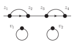
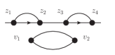
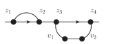
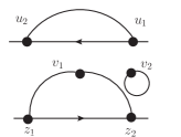
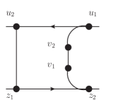
All possible contractions for ⟨ ρ z 1 a ρ z 2 b ρ z 3 c ρ z 4 d ρ v 1 e ρ v 1 e ρ v 2 f ρ v 2 f ⟩ delimited-⟨⟩ superscript subscript 𝜌 subscript 𝑧 1 𝑎 superscript subscript 𝜌 subscript 𝑧 2 𝑏 superscript subscript 𝜌 subscript 𝑧 3 𝑐 superscript subscript 𝜌 subscript 𝑧 4 𝑑 superscript subscript 𝜌 subscript 𝑣 1 𝑒 superscript subscript 𝜌 subscript 𝑣 1 𝑒 superscript subscript 𝜌 subscript 𝑣 2 𝑓 superscript subscript 𝜌 subscript 𝑣 2 𝑓 \langle\rho_{z_{1}}^{a}\rho_{z_{2}}^{b}\rho_{z_{3}}^{c}\rho_{z_{4}}^{d}\rho_{v_{1}}^{e}\rho_{v_{1}}^{e}\rho_{v_{2}}^{f}\rho_{v_{2}}^{f}\rangle 3
Figure 3: Order g 8 / κ 4 superscript 𝑔 8 subscript 𝜅 4 g^{8}/\kappa_{4} ⟨ V ⟩ delimited-⟨⟩ 𝑉 \langle V\rangle
The disconnected diagrams 3a
− \displaystyle- g 8 8 ( t a t a ) 2 [ ∫ − ∞ ∞ 𝑑 z − μ 2 ( z − ) ] 2 [ ∫ d 2 𝕫 ⟂ G 0 2 ( 𝕩 ⟂ − 𝕫 ⟂ ) ] 2 superscript 𝑔 8 8 superscript superscript 𝑡 𝑎 subscript 𝑡 𝑎 2 superscript delimited-[] superscript subscript differential-d superscript 𝑧 superscript 𝜇 2 superscript 𝑧 2 superscript delimited-[] superscript 𝑑 2 subscript 𝕫 perpendicular-to superscript subscript 𝐺 0 2 subscript 𝕩 perpendicular-to subscript 𝕫 perpendicular-to 2 \displaystyle\frac{g^{8}}{8}\left(t^{a}t_{a}\right)^{2}\left[\int_{-\infty}^{\infty}dz^{-}\mu^{2}(z^{-})\right]^{2}\left[\int d^{2}\mathbb{z}_{\perp}G_{0}^{2}(\mathbb{x}_{\perp}-\mathbb{z}_{\perp})\right]^{2} (37)
× 1 κ 4 N s Δ 𝕧 ⟂ [ ( N c 2 − 1 ) 2 [ ∫ − ∞ ∞ 𝑑 v − μ 2 ( v − ) ] 2 + 2 ( N c 2 − 1 ) ∫ − ∞ ∞ 𝑑 v − μ 4 ( v − ) ] , absent 1 subscript 𝜅 4 subscript 𝑁 𝑠 Δ subscript 𝕧 perpendicular-to delimited-[] superscript superscript subscript 𝑁 𝑐 2 1 2 superscript delimited-[] subscript superscript differential-d superscript 𝑣 superscript 𝜇 2 superscript 𝑣 2 2 superscript subscript 𝑁 𝑐 2 1 subscript superscript differential-d superscript 𝑣 superscript 𝜇 4 superscript 𝑣 \displaystyle\times\frac{1}{\kappa_{4}}\frac{N_{s}}{\Delta\mathbb{v}_{\perp}}\left[(N_{c}^{2}-1)^{2}\left[\int^{\infty}_{-\infty}dv^{-}\mu^{2}(v^{-})\right]^{2}+2~{}(N_{c}^{2}-1)\int^{\infty}_{-\infty}dv^{-}\mu^{4}(v^{-})\right]~{},
which will cancel the normalization factor.
The connected diagrams from fig. 3b μ 2 ( z − ) superscript 𝜇 2 superscript 𝑧 \mu^{2}(z^{-}) μ ~ 2 ( z − ) superscript ~ 𝜇 2 superscript 𝑧 \tilde{\mu}^{2}(z^{-})
[ ∫ − ∞ ∞ 𝑑 z − μ ~ 2 ( z − ) ] 2 superscript delimited-[] superscript subscript differential-d superscript 𝑧 superscript ~ 𝜇 2 superscript 𝑧 2 \displaystyle\left[\int_{-\infty}^{\infty}dz^{-}\tilde{\mu}^{2}(z^{-})\right]^{2} = \displaystyle= [ ∫ − ∞ ∞ 𝑑 z − μ 2 ( z − ) ] 2 superscript delimited-[] subscript superscript differential-d superscript 𝑧 superscript 𝜇 2 superscript 𝑧 2 \displaystyle\left[\int^{\infty}_{-\infty}dz^{-}\mu^{2}(z^{-})\right]^{2} (38)
− 8 κ 4 Δ 𝕧 ⟂ [ ( N c 2 − 1 ) [ ∫ − ∞ ∞ 𝑑 z − μ 2 ( z − ) ] 2 ∫ − ∞ ∞ 𝑑 v − μ 4 ( v − ) + 2 ∫ − ∞ ∞ 𝑑 z − μ 2 ( z − ) ∫ − ∞ ∞ 𝑑 v − μ 6 ( v − ) ] . 8 subscript 𝜅 4 Δ subscript 𝕧 perpendicular-to delimited-[] superscript subscript 𝑁 𝑐 2 1 superscript delimited-[] superscript subscript differential-d superscript 𝑧 superscript 𝜇 2 superscript 𝑧 2 superscript subscript differential-d superscript 𝑣 superscript 𝜇 4 superscript 𝑣 2 superscript subscript differential-d superscript 𝑧 superscript 𝜇 2 superscript 𝑧 superscript subscript differential-d superscript 𝑣 superscript 𝜇 6 superscript 𝑣 \displaystyle-\frac{8}{\kappa_{4}\Delta\mathbb{v}_{\perp}}\left[(N_{c}^{2}-1)\left[\int_{-\infty}^{\infty}dz^{-}\mu^{2}(z^{-})\right]^{2}\int_{-\infty}^{\infty}dv^{-}\mu^{4}(v^{-})+2\int_{-\infty}^{\infty}dz^{-}\mu^{2}(z^{-})\int_{-\infty}^{\infty}dv^{-}\mu^{6}(v^{-})\right]~{}.
Finally, the diagrams 3c
− g 8 κ 4 ( t a t a ) 2 [ ∫ − ∞ ∞ 𝑑 z − μ 4 ( z − ) ] 2 ∫ d 2 𝕫 ⟂ G 0 4 ( 𝕩 ⟂ − 𝕫 ⟂ ) . superscript 𝑔 8 subscript 𝜅 4 superscript superscript 𝑡 𝑎 subscript 𝑡 𝑎 2 superscript delimited-[] superscript subscript differential-d superscript 𝑧 superscript 𝜇 4 superscript 𝑧 2 superscript 𝑑 2 subscript 𝕫 perpendicular-to superscript subscript 𝐺 0 4 subscript 𝕩 perpendicular-to subscript 𝕫 perpendicular-to -\frac{g^{8}}{\kappa_{4}}\left(t^{a}t_{a}\right)^{2}\left[\int_{-\infty}^{\infty}dz^{-}\mu^{4}(z^{-})\right]^{2}\int d^{2}\mathbb{z}_{\perp}G_{0}^{4}(\mathbb{x}_{\perp}-\mathbb{z}_{\perp})~{}~{}. (39)
That leads us to the complete 𝒪 ( g 8 ) 𝒪 superscript 𝑔 8 \mathcal{O}(g^{8}) ⟨ V ( x ⟂ ) ⟩ delimited-⟨⟩ 𝑉 subscript 𝑥 perpendicular-to \langle V(x_{\perp})\rangle
g 8 8 ( t a t a ) 2 [ ∫ − ∞ ∞ 𝑑 z − μ ~ 2 ( z − ) ] 2 [ ∫ d 2 𝕫 ⟂ G 0 2 ( 𝕩 ⟂ − 𝕫 ⟂ ) ] 2 superscript 𝑔 8 8 superscript superscript 𝑡 𝑎 subscript 𝑡 𝑎 2 superscript delimited-[] superscript subscript differential-d superscript 𝑧 superscript ~ 𝜇 2 superscript 𝑧 2 superscript delimited-[] superscript 𝑑 2 subscript 𝕫 perpendicular-to superscript subscript 𝐺 0 2 subscript 𝕩 perpendicular-to subscript 𝕫 perpendicular-to 2 \displaystyle\frac{g^{8}}{8}\left(t^{a}t_{a}\right)^{2}~{}\left[\int_{-\infty}^{\infty}dz^{-}\tilde{\mu}^{2}(z^{-})\right]^{2}~{}\left[\int d^{2}\mathbb{z}_{\perp}G_{0}^{2}(\mathbb{x}_{\perp}-\mathbb{z}_{\perp})\right]^{2} (40)
− \displaystyle- g 8 κ 4 ( t a t a ) 2 [ ∫ − ∞ ∞ 𝑑 z − μ 4 ( z − ) ] 2 ∫ d 2 𝕫 ⟂ G 0 4 ( 𝕩 ⟂ − 𝕫 ⟂ ) . superscript 𝑔 8 subscript 𝜅 4 superscript superscript 𝑡 𝑎 subscript 𝑡 𝑎 2 superscript delimited-[] superscript subscript differential-d superscript 𝑧 superscript 𝜇 4 superscript 𝑧 2 superscript 𝑑 2 subscript 𝕫 perpendicular-to superscript subscript 𝐺 0 4 subscript 𝕩 perpendicular-to subscript 𝕫 perpendicular-to \displaystyle\frac{g^{8}}{\kappa_{4}}\left(t^{a}t_{a}\right)^{2}\left[\int_{-\infty}^{\infty}dz^{-}\mu^{4}(z^{-})\right]^{2}\int d^{2}\mathbb{z}_{\perp}G_{0}^{4}(\mathbb{x}_{\perp}-\mathbb{z}_{\perp})~{}.
The expectation value of V † ( 𝕪 ⟂ ) superscript 𝑉 † subscript 𝕪 perpendicular-to V^{\dagger}(\mathbb{y}_{\perp}) 𝕩 ⟂ → 𝕪 ⟂ → subscript 𝕩 perpendicular-to subscript 𝕪 perpendicular-to \mathbb{x}_{\perp}\to\mathbb{y}_{\perp}
I.3.2 g 6 superscript 𝑔 6 g^{6} V ( 𝕩 ⟂ ) 𝑉 subscript 𝕩 perpendicular-to V(\mathbb{x}_{\perp}) × \times g 2 superscript 𝑔 2 g^{2} V † ( 𝕪 ⟂ ) superscript 𝑉 † subscript 𝕪 perpendicular-to V^{\dagger}(\mathbb{y}_{\perp})
Next is the mixed term obtained when multiplying the g 6 superscript 𝑔 6 g^{6} x 𝑥 x g 2 superscript 𝑔 2 g^{2} y 𝑦 y
− g 8 2 ( t a t a ) 2 [ ∫ − ∞ ∞ 𝑑 z − μ 2 ( z − ) ] 2 ∫ d 2 𝕫 ⟂ G 0 2 ( 𝕩 ⟂ − 𝕫 ⟂ ) ∫ d 2 𝕦 ⟂ G 0 ( 𝕩 ⟂ − 𝕦 ⟂ ) G 0 ( 𝕪 ⟂ − 𝕦 ⟂ ) . superscript 𝑔 8 2 superscript superscript 𝑡 𝑎 subscript 𝑡 𝑎 2 superscript delimited-[] superscript subscript differential-d superscript 𝑧 superscript 𝜇 2 superscript 𝑧 2 superscript 𝑑 2 subscript 𝕫 perpendicular-to superscript subscript 𝐺 0 2 subscript 𝕩 perpendicular-to subscript 𝕫 perpendicular-to superscript 𝑑 2 subscript 𝕦 perpendicular-to subscript 𝐺 0 subscript 𝕩 perpendicular-to subscript 𝕦 perpendicular-to subscript 𝐺 0 subscript 𝕪 perpendicular-to subscript 𝕦 perpendicular-to -\frac{g^{8}}{2}\left(t^{a}t_{a}\right)^{2}\left[\int_{-\infty}^{\infty}dz^{-}\mu^{2}(z^{-})\right]^{2}\int d^{2}\mathbb{z}_{\perp}G_{0}^{2}(\mathbb{x}_{\perp}-\mathbb{z}_{\perp})\int d^{2}\mathbb{u}_{\perp}G_{0}(\mathbb{x}_{\perp}-\mathbb{u}_{\perp})G_{0}(\mathbb{y}_{\perp}-\mathbb{u}_{\perp})~{}. (41)
The correction is:
+ \displaystyle+ g 8 κ 4 ∫ d 2 𝕫 ⟂ 1 d 2 𝕫 ⟂ 2 d 2 𝕫 ⟂ 3 G 0 ( 𝕩 ⟂ − 𝕫 ⟂ 1 ) G 0 ( 𝕩 ⟂ − 𝕫 ⟂ 2 ) G 0 ( 𝕩 ⟂ − 𝕫 ⟂ 3 ) ∫ d 2 𝕦 ⟂ 1 G 0 ( 𝕪 ⟂ − 𝕦 ⟂ 1 ) superscript 𝑔 8 subscript 𝜅 4 superscript 𝑑 2 subscript 𝕫 perpendicular-to absent 1 superscript 𝑑 2 subscript 𝕫 perpendicular-to absent 2 superscript 𝑑 2 subscript 𝕫 perpendicular-to absent 3 subscript 𝐺 0 subscript 𝕩 perpendicular-to subscript 𝕫 perpendicular-to absent 1 subscript 𝐺 0 subscript 𝕩 perpendicular-to subscript 𝕫 perpendicular-to absent 2 subscript 𝐺 0 subscript 𝕩 perpendicular-to subscript 𝕫 perpendicular-to absent 3 superscript 𝑑 2 subscript 𝕦 perpendicular-to absent 1 subscript 𝐺 0 subscript 𝕪 perpendicular-to subscript 𝕦 perpendicular-to absent 1 \displaystyle\frac{g^{8}}{\kappa_{4}}\int d^{2}\mathbb{z}_{\perp 1}d^{2}\mathbb{z}_{\perp 2}d^{2}\mathbb{z}_{\perp 3}G_{0}(\mathbb{x}_{\perp}-\mathbb{z}_{\perp 1})G_{0}(\mathbb{x}_{\perp}-\mathbb{z}_{\perp 2})G_{0}(\mathbb{x}_{\perp}-\mathbb{z}_{\perp 3})\int d^{2}\mathbb{u}_{\perp 1}G_{0}(\mathbb{y}_{\perp}-\mathbb{u}_{\perp 1}) (42)
× ∫ d 2 𝕧 ⟂ ∫ − ∞ ∞ d z 1 − ∫ z 1 − ∞ d z 2 − ∫ z 2 − ∞ d z 3 − ∫ − ∞ ∞ d u 1 − ∫ − ∞ ∞ d v 1 − ∫ − ∞ ∞ d v 2 − \displaystyle\times\int d^{2}\mathbb{v}_{\perp}\int_{-\infty}^{\infty}dz_{1}^{-}\int_{z_{1}^{-}}^{\infty}dz_{2}^{-}\int_{z_{2}^{-}}^{\infty}dz_{3}^{-}\int_{-\infty}^{\infty}du_{1}^{-}\int_{-\infty}^{\infty}dv_{1}^{-}\int_{-\infty}^{\infty}dv_{2}^{-}
× ⟨ ρ z 1 a ρ z 2 b ρ z 3 c ρ u 1 d ρ v 1 e ρ v 1 e ρ v 2 f ρ v 2 f ⟩ t a t b t c t d . absent delimited-⟨⟩ superscript subscript 𝜌 subscript 𝑧 1 𝑎 superscript subscript 𝜌 subscript 𝑧 2 𝑏 superscript subscript 𝜌 subscript 𝑧 3 𝑐 superscript subscript 𝜌 subscript 𝑢 1 𝑑 superscript subscript 𝜌 subscript 𝑣 1 𝑒 superscript subscript 𝜌 subscript 𝑣 1 𝑒 superscript subscript 𝜌 subscript 𝑣 2 𝑓 superscript subscript 𝜌 subscript 𝑣 2 𝑓 superscript 𝑡 𝑎 superscript 𝑡 𝑏 superscript 𝑡 𝑐 superscript 𝑡 𝑑 \displaystyle\times\langle\rho_{z_{1}}^{a}\rho_{z_{2}}^{b}\rho_{z_{3}}^{c}\rho_{u_{1}}^{d}\rho_{v_{1}}^{e}\rho_{v_{1}}^{e}\rho_{v_{2}}^{f}\rho_{v_{2}}^{f}\rangle t^{a}t^{b}t^{c}t^{d}~{}.
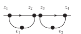
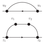
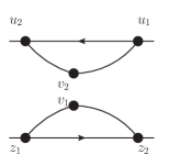
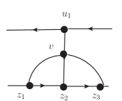
The possible contractions are given in fig. 4
Figure 4: V ( x ⟂ ) V † ( y ⟂ ) 𝑉 subscript 𝑥 perpendicular-to superscript 𝑉 † subscript 𝑦 perpendicular-to V(x_{\perp})V^{\dagger}(y_{\perp}) g 8 / κ 4 superscript 𝑔 8 subscript 𝜅 4 g^{8}/\kappa_{4} g 6 superscript 𝑔 6 g^{6} V ( 𝕩 ⟂ ) 𝑉 subscript 𝕩 perpendicular-to V(\mathbb{x}_{\perp}) × \times g 2 superscript 𝑔 2 g^{2} V † ( 𝕪 ⟂ ) superscript 𝑉 † subscript 𝕪 perpendicular-to V^{\dagger}(\mathbb{y}_{\perp})
As before, the disconnected diagrams 4a 4b μ 2 superscript 𝜇 2 \mu^{2} μ ~ 2 superscript ~ 𝜇 2 \tilde{\mu}^{2} 4c
− g 8 2 ( t a t a ) 2 [ ∫ − ∞ ∞ 𝑑 z − μ ~ 2 ( z − ) ] 2 ∫ d 2 𝕫 ⟂ G 0 2 ( 𝕩 ⟂ − 𝕫 ⟂ ) ∫ d 2 𝕦 ⟂ G 0 ( 𝕩 ⟂ − 𝕦 ⟂ ) G 0 ( 𝕪 ⟂ − 𝕦 ⟂ ) superscript 𝑔 8 2 superscript superscript 𝑡 𝑎 subscript 𝑡 𝑎 2 superscript delimited-[] superscript subscript differential-d superscript 𝑧 superscript ~ 𝜇 2 superscript 𝑧 2 superscript 𝑑 2 subscript 𝕫 perpendicular-to superscript subscript 𝐺 0 2 subscript 𝕩 perpendicular-to subscript 𝕫 perpendicular-to superscript 𝑑 2 subscript 𝕦 perpendicular-to subscript 𝐺 0 subscript 𝕩 perpendicular-to subscript 𝕦 perpendicular-to subscript 𝐺 0 subscript 𝕪 perpendicular-to subscript 𝕦 perpendicular-to \displaystyle-\frac{g^{8}}{2}\left(t^{a}t_{a}\right)^{2}~{}\left[\int_{-\infty}^{\infty}dz^{-}\tilde{\mu}^{2}(z^{-})\right]^{2}~{}\int d^{2}\mathbb{z}_{\perp}G_{0}^{2}(\mathbb{x}_{\perp}-\mathbb{z}_{\perp})\int d^{2}\mathbb{u}_{\perp}G_{0}(\mathbb{x}_{\perp}-\mathbb{u}_{\perp})G_{0}(\mathbb{y}_{\perp}-\mathbb{u}_{\perp})
+ 4 g 8 κ 4 ( t a t a ) 2 [ ∫ − ∞ ∞ 𝑑 z − μ 4 ( z − ) ] 2 ∫ d 2 𝕫 ⟂ G 0 3 ( 𝕩 ⟂ − 𝕫 ⟂ ) G 0 ( 𝕪 ⟂ − 𝕫 ⟂ ) . 4 superscript 𝑔 8 subscript 𝜅 4 superscript superscript 𝑡 𝑎 subscript 𝑡 𝑎 2 superscript delimited-[] superscript subscript differential-d superscript 𝑧 superscript 𝜇 4 superscript 𝑧 2 superscript 𝑑 2 subscript 𝕫 perpendicular-to superscript subscript 𝐺 0 3 subscript 𝕩 perpendicular-to subscript 𝕫 perpendicular-to subscript 𝐺 0 subscript 𝕪 perpendicular-to subscript 𝕫 perpendicular-to \displaystyle+4~{}\frac{g^{8}}{\kappa_{4}}\left(t^{a}t_{a}\right)^{2}\left[\int_{-\infty}^{\infty}dz^{-}\mu^{4}(z^{-})\right]^{2}\int d^{2}\mathbb{z}_{\perp}G_{0}^{3}(\mathbb{x}_{\perp}-\mathbb{z}_{\perp})G_{0}(\mathbb{y}_{\perp}-\mathbb{z}_{\perp})~{}. (43)
Once again, a similar contribution (with 𝕩 ⟂ ↔ 𝕪 ⟂ ↔ subscript 𝕩 perpendicular-to subscript 𝕪 perpendicular-to {\mathbb{x}_{\perp}}\leftrightarrow{\mathbb{y}_{\perp}} V ( 𝕩 ⟂ ) 𝑉 subscript 𝕩 perpendicular-to V(\mathbb{x}_{\perp}) 𝒪 ( g 2 ) 𝒪 superscript 𝑔 2 \mathcal{O}(g^{2}) V † ( 𝕪 ⟂ ) superscript 𝑉 † subscript 𝕪 perpendicular-to V^{\dagger}(\mathbb{y}_{\perp}) g 6 superscript 𝑔 6 g^{6}
I.3.3 g 4 superscript 𝑔 4 g^{4} V ( 𝕩 ⟂ ) 𝑉 subscript 𝕩 perpendicular-to V(\mathbb{x}_{\perp}) × \times g 4 superscript 𝑔 4 g^{4} V † ( 𝕪 ⟂ ) superscript 𝑉 † subscript 𝕪 perpendicular-to V^{\dagger}(\mathbb{y}_{\perp})
The last term to consider is the one obtained when multiplying
𝒪 ( g 4 ) 𝒪 superscript 𝑔 4 \mathcal{O}(g^{4}) x 𝑥 x 𝒪 ( g 4 ) 𝒪 superscript 𝑔 4 \mathcal{O}(g^{4}) y 𝑦 y
g 8 4 ( t a t a ) 2 [ ∫ − ∞ ∞ 𝑑 z − μ 2 ( z − ) ] 2 ∫ d 2 𝕫 ⟂ G 0 2 ( 𝕩 ⟂ − 𝕫 ⟂ ) ∫ d 2 𝕦 ⟂ G 0 2 ( 𝕪 ⟂ − 𝕦 ⟂ ) superscript 𝑔 8 4 superscript superscript 𝑡 𝑎 subscript 𝑡 𝑎 2 superscript delimited-[] superscript subscript differential-d superscript 𝑧 superscript 𝜇 2 superscript 𝑧 2 superscript 𝑑 2 subscript 𝕫 perpendicular-to superscript subscript 𝐺 0 2 subscript 𝕩 perpendicular-to subscript 𝕫 perpendicular-to superscript 𝑑 2 subscript 𝕦 perpendicular-to superscript subscript 𝐺 0 2 subscript 𝕪 perpendicular-to subscript 𝕦 perpendicular-to \displaystyle\frac{g^{8}}{4}\left(t^{a}t_{a}\right)^{2}\left[\int_{-\infty}^{\infty}dz^{-}\mu^{2}(z^{-})\right]^{2}\int d^{2}\mathbb{z}_{\perp}G_{0}^{2}(\mathbb{x}_{\perp}-\mathbb{z}_{\perp})\int d^{2}\mathbb{u}_{\perp}G_{0}^{2}(\mathbb{y}_{\perp}-\mathbb{u}_{\perp})
+ g 8 2 ( t a t a ) 2 [ ∫ − ∞ ∞ 𝑑 z − μ 2 ( z − ) ] 2 [ ∫ d 2 𝕫 ⟂ G 0 ( 𝕩 ⟂ − 𝕫 ⟂ ) G 0 ( 𝕪 ⟂ − 𝕦 ⟂ ) ] 2 . superscript 𝑔 8 2 superscript superscript 𝑡 𝑎 subscript 𝑡 𝑎 2 superscript delimited-[] superscript subscript differential-d superscript 𝑧 superscript 𝜇 2 superscript 𝑧 2 superscript delimited-[] superscript 𝑑 2 subscript 𝕫 perpendicular-to subscript 𝐺 0 subscript 𝕩 perpendicular-to subscript 𝕫 perpendicular-to subscript 𝐺 0 subscript 𝕪 perpendicular-to subscript 𝕦 perpendicular-to 2 \displaystyle+\frac{g^{8}}{2}\left(t^{a}t_{a}\right)^{2}\left[\int_{-\infty}^{\infty}dz^{-}\mu^{2}(z^{-})\right]^{2}\left[\int d^{2}\mathbb{z}_{\perp}G_{0}(\mathbb{x}_{\perp}-\mathbb{z}_{\perp})G_{0}(\mathbb{y}_{\perp}-\mathbb{u}_{\perp})\right]^{2}~{}. (44)
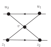
For the quartic action we have to add
− \displaystyle- g 8 κ 4 ∫ d 2 𝕫 ⟂ 1 d 2 𝕫 ⟂ 2 G 0 ( 𝕩 ⟂ − 𝕫 ⟂ 1 ) G 0 ( 𝕩 ⟂ − 𝕫 ⟂ 2 ) ∫ d 2 𝕦 ⟂ 1 d 2 𝕦 ⟂ 2 G 0 ( 𝕪 ⟂ − 𝕦 ⟂ 1 ) G 0 ( 𝕪 ⟂ − 𝕦 ⟂ 2 ) superscript 𝑔 8 subscript 𝜅 4 superscript 𝑑 2 subscript 𝕫 perpendicular-to absent 1 superscript 𝑑 2 subscript 𝕫 perpendicular-to absent 2 subscript 𝐺 0 subscript 𝕩 perpendicular-to subscript 𝕫 perpendicular-to absent 1 subscript 𝐺 0 subscript 𝕩 perpendicular-to subscript 𝕫 perpendicular-to absent 2 superscript 𝑑 2 subscript 𝕦 perpendicular-to absent 1 superscript 𝑑 2 subscript 𝕦 perpendicular-to absent 2 subscript 𝐺 0 subscript 𝕪 perpendicular-to subscript 𝕦 perpendicular-to absent 1 subscript 𝐺 0 subscript 𝕪 perpendicular-to subscript 𝕦 perpendicular-to absent 2 \displaystyle\frac{g^{8}}{\kappa_{4}}\int d^{2}\mathbb{z}_{\perp 1}d^{2}\mathbb{z}_{\perp 2}G_{0}(\mathbb{x}_{\perp}-\mathbb{z}_{\perp 1})G_{0}(\mathbb{x}_{\perp}-\mathbb{z}_{\perp 2})\int d^{2}\mathbb{u}_{\perp 1}d^{2}\mathbb{u}_{\perp 2}G_{0}(\mathbb{y}_{\perp}-\mathbb{u}_{\perp 1})G_{0}(\mathbb{y}_{\perp}-\mathbb{u}_{\perp 2}) (45)
× ∫ d 2 𝕧 ⟂ ∫ − ∞ ∞ d z 1 − ∫ z 1 − ∞ d z 2 − ∫ − ∞ ∞ d u 1 − ∫ − ∞ u 1 − d u 2 − ∫ − ∞ ∞ d v 1 − ∫ − ∞ ∞ d v 2 − \displaystyle\times\int d^{2}\mathbb{v}_{\perp}\int_{-\infty}^{\infty}dz_{1}^{-}\int_{z_{1}^{-}}^{\infty}dz_{2}^{-}\int_{-\infty}^{\infty}du_{1}^{-}\int_{-\infty}^{u_{1}^{-}}du_{2}^{-}\int_{-\infty}^{\infty}dv_{1}^{-}\int_{-\infty}^{\infty}dv_{2}^{-}
× ⟨ ρ z 1 a ρ z 2 b ρ u 1 c ρ u 2 d ρ v 1 e ρ v 1 e ρ v 2 f ρ v 2 f ⟩ t a t b t c t d . absent delimited-⟨⟩ superscript subscript 𝜌 subscript 𝑧 1 𝑎 superscript subscript 𝜌 subscript 𝑧 2 𝑏 superscript subscript 𝜌 subscript 𝑢 1 𝑐 superscript subscript 𝜌 subscript 𝑢 2 𝑑 superscript subscript 𝜌 subscript 𝑣 1 𝑒 superscript subscript 𝜌 subscript 𝑣 1 𝑒 superscript subscript 𝜌 subscript 𝑣 2 𝑓 superscript subscript 𝜌 subscript 𝑣 2 𝑓 superscript 𝑡 𝑎 superscript 𝑡 𝑏 superscript 𝑡 𝑐 superscript 𝑡 𝑑 \displaystyle\times\langle\rho_{z_{1}}^{a}\rho_{z_{2}}^{b}\rho_{u_{1}}^{c}\rho_{u_{2}}^{d}\rho_{v_{1}}^{e}\rho_{v_{1}}^{e}\rho_{v_{2}}^{f}\rho_{v_{2}}^{f}\rangle t^{a}t^{b}t^{c}t^{d}~{}.
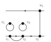
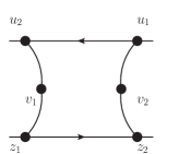
Figure 5: Expectation value of
V ( 𝕩 ⟂ ) 𝑉 subscript 𝕩 perpendicular-to V(\mathbb{x}_{\perp}) g 4 superscript 𝑔 4 g^{4} V ( 𝕪 ⟂ ) 𝑉 subscript 𝕪 perpendicular-to V(\mathbb{y}_{\perp}) g 4 superscript 𝑔 4 g^{4}
Following the same procedure as before, the diagrams from
fig. 5
g 8 4 ( t a t a ) 2 [ ∫ − ∞ ∞ 𝑑 z − μ ~ 2 ( z − ) ] 2 ∫ d 2 𝕫 ⟂ G 0 2 ( 𝕩 ⟂ − 𝕫 ⟂ ) ∫ d 2 𝕦 ⟂ G 0 2 ( 𝕪 ⟂ − 𝕦 ⟂ ) superscript 𝑔 8 4 superscript superscript 𝑡 𝑎 subscript 𝑡 𝑎 2 superscript delimited-[] superscript subscript differential-d superscript 𝑧 superscript ~ 𝜇 2 superscript 𝑧 2 superscript 𝑑 2 subscript 𝕫 perpendicular-to superscript subscript 𝐺 0 2 subscript 𝕩 perpendicular-to subscript 𝕫 perpendicular-to superscript 𝑑 2 subscript 𝕦 perpendicular-to superscript subscript 𝐺 0 2 subscript 𝕪 perpendicular-to subscript 𝕦 perpendicular-to \displaystyle\frac{g^{8}}{4}\left(t^{a}t_{a}\right)^{2}~{}\left[\int_{-\infty}^{\infty}dz^{-}\tilde{\mu}^{2}(z^{-})\right]^{2}~{}\int d^{2}\mathbb{z}_{\perp}G_{0}^{2}(\mathbb{x}_{\perp}-\mathbb{z}_{\perp})\int d^{2}\mathbb{u}_{\perp}G_{0}^{2}(\mathbb{y}_{\perp}-\mathbb{u}_{\perp})
+ g 8 2 ( t a t a ) 2 [ ∫ − ∞ ∞ 𝑑 z − μ ~ 2 ( z − ) ] 2 [ ∫ d 2 𝕫 ⟂ G 0 ( 𝕩 ⟂ − 𝕫 ⟂ ) G 0 ( 𝕪 ⟂ − 𝕦 ⟂ ) ] 2 superscript 𝑔 8 2 superscript superscript 𝑡 𝑎 subscript 𝑡 𝑎 2 superscript delimited-[] superscript subscript differential-d superscript 𝑧 superscript ~ 𝜇 2 superscript 𝑧 2 superscript delimited-[] superscript 𝑑 2 subscript 𝕫 perpendicular-to subscript 𝐺 0 subscript 𝕩 perpendicular-to subscript 𝕫 perpendicular-to subscript 𝐺 0 subscript 𝕪 perpendicular-to subscript 𝕦 perpendicular-to 2 \displaystyle+\frac{g^{8}}{2}\left(t^{a}t_{a}\right)^{2}~{}\left[\int_{-\infty}^{\infty}dz^{-}\tilde{\mu}^{2}(z^{-})\right]^{2}~{}\left[\int d^{2}\mathbb{z}_{\perp}G_{0}(\mathbb{x}_{\perp}-\mathbb{z}_{\perp})G_{0}(\mathbb{y}_{\perp}-\mathbb{u}_{\perp})\right]^{2}
− 6 g 8 κ 4 ( t a t a ) 2 [ ∫ − ∞ ∞ 𝑑 z − μ 4 ( z − ) ] 2 ∫ d 2 𝕫 ⟂ G 0 2 ( 𝕩 ⟂ − 𝕫 ⟂ ) G 0 2 ( 𝕪 ⟂ − 𝕫 ⟂ ) . 6 superscript 𝑔 8 subscript 𝜅 4 superscript superscript 𝑡 𝑎 subscript 𝑡 𝑎 2 superscript delimited-[] superscript subscript differential-d superscript 𝑧 superscript 𝜇 4 superscript 𝑧 2 superscript 𝑑 2 subscript 𝕫 perpendicular-to superscript subscript 𝐺 0 2 subscript 𝕩 perpendicular-to subscript 𝕫 perpendicular-to superscript subscript 𝐺 0 2 subscript 𝕪 perpendicular-to subscript 𝕫 perpendicular-to \displaystyle-6~{}\frac{g^{8}}{\kappa_{4}}\left(t^{a}t_{a}\right)^{2}\left[\int_{-\infty}^{\infty}dz^{-}\mu^{4}(z^{-})\right]^{2}\int d^{2}\mathbb{z}_{\perp}G_{0}^{2}(\mathbb{x}_{\perp}-\mathbb{z}_{\perp})G_{0}^{2}(\mathbb{y}_{\perp}-\mathbb{z}_{\perp})~{}. (46)
I.3.4 Complete order g 8 superscript 𝑔 8 g^{8}
Combining eqs. (40 x ⟂ ↔ y ⟂ ↔ subscript 𝑥 perpendicular-to subscript 𝑦 perpendicular-to x_{\perp}\leftrightarrow y_{\perp} I.3.2 x ⟂ ↔ y ⟂ ↔ subscript 𝑥 perpendicular-to subscript 𝑦 perpendicular-to x_{\perp}\leftrightarrow y_{\perp} I.3.3 g 8 superscript 𝑔 8 g^{8}
1 2 ( g 4 ( t a t a ) 2 ) 2 [ ∫ − ∞ ∞ 𝑑 z − μ ~ 2 ( z − ) ] 2 [ ∫ d 2 𝕫 ⟂ [ G 0 ( 𝕩 ⟂ − 𝕫 ⟂ ) − G 0 ( 𝕪 ⟂ − 𝕫 ⟂ ) ] 2 ] 2 1 2 superscript superscript 𝑔 4 superscript 𝑡 𝑎 subscript 𝑡 𝑎 2 2 superscript delimited-[] superscript subscript differential-d superscript 𝑧 superscript ~ 𝜇 2 superscript 𝑧 2 superscript delimited-[] superscript 𝑑 2 subscript 𝕫 perpendicular-to superscript delimited-[] subscript 𝐺 0 subscript 𝕩 perpendicular-to subscript 𝕫 perpendicular-to subscript 𝐺 0 subscript 𝕪 perpendicular-to subscript 𝕫 perpendicular-to 2 2 \displaystyle\frac{1}{2}\left(\frac{g^{4}\left(t^{a}t_{a}\right)}{2}\right)^{2}~{}\left[\int_{-\infty}^{\infty}dz^{-}\tilde{\mu}^{2}(z^{-})\right]^{2}~{}\left[\int d^{2}\mathbb{z}_{\perp}\left[G_{0}(\mathbb{x}_{\perp}-\mathbb{z}_{\perp})-G_{0}(\mathbb{y}_{\perp}-\mathbb{z}_{\perp})\right]^{2}\right]^{2}
− g 8 κ 4 ( t a t a ) 2 [ ∫ − ∞ ∞ 𝑑 z − μ 4 ( z − ) ] 2 ∫ d 2 𝕫 ⟂ [ G 0 ( 𝕩 ⟂ − 𝕫 ⟂ ) − G 0 ( 𝕪 ⟂ − 𝕫 ⟂ ) ] 4 . superscript 𝑔 8 subscript 𝜅 4 superscript superscript 𝑡 𝑎 subscript 𝑡 𝑎 2 superscript delimited-[] superscript subscript differential-d superscript 𝑧 superscript 𝜇 4 superscript 𝑧 2 superscript 𝑑 2 subscript 𝕫 perpendicular-to superscript delimited-[] subscript 𝐺 0 subscript 𝕩 perpendicular-to subscript 𝕫 perpendicular-to subscript 𝐺 0 subscript 𝕪 perpendicular-to subscript 𝕫 perpendicular-to 4 \displaystyle-\frac{g^{8}}{\kappa_{4}}\left(t^{a}t_{a}\right)^{2}\left[\int_{-\infty}^{\infty}dz^{-}\mu^{4}(z^{-})\right]^{2}\int d^{2}\mathbb{z}_{\perp}\left[G_{0}(\mathbb{x}_{\perp}-\mathbb{z}_{\perp})-G_{0}(\mathbb{y}_{\perp}-\mathbb{z}_{\perp})\right]^{4}~{}.
Note that this again vanishes as 𝕪 ⟂ → 𝕩 ⟂ → subscript 𝕪 perpendicular-to subscript 𝕩 perpendicular-to \mathbb{y}_{\perp}\to\mathbb{x}_{\perp}
I.4 Complete expectation value of the dipole operator
Adding together the terms of order 1, g 4 superscript 𝑔 4 g^{4} g 8 superscript 𝑔 8 g^{8}
D ( x ⟂ − y ⟂ ) 𝐷 subscript 𝑥 perpendicular-to subscript 𝑦 perpendicular-to \displaystyle D(x_{\perp}-y_{\perp}) ≡ \displaystyle\equiv ⟨ 1 N c tr V ( 𝕩 ⟂ ) V † ( 𝕪 ⟂ ) ⟩ = delimited-⟨⟩ 1 subscript 𝑁 𝑐 tr 𝑉 subscript 𝕩 perpendicular-to superscript 𝑉 † subscript 𝕪 perpendicular-to absent \displaystyle\langle\frac{1}{N_{c}}{\rm tr}~{}V(\mathbb{x}_{\perp})V^{\dagger}(\mathbb{y}_{\perp})\rangle=
1 1 \displaystyle 1 − \displaystyle- g 4 2 C F ∫ − ∞ ∞ 𝑑 z − μ ~ 2 ( z − ) ∫ d 2 𝕫 ⟂ [ G 0 ( 𝕩 ⟂ − 𝕫 ⟂ ) − G 0 ( 𝕪 ⟂ − 𝕫 ⟂ ) ] 2 superscript 𝑔 4 2 subscript 𝐶 𝐹 superscript subscript differential-d superscript 𝑧 superscript ~ 𝜇 2 superscript 𝑧 superscript 𝑑 2 subscript 𝕫 perpendicular-to superscript delimited-[] subscript 𝐺 0 subscript 𝕩 perpendicular-to subscript 𝕫 perpendicular-to subscript 𝐺 0 subscript 𝕪 perpendicular-to subscript 𝕫 perpendicular-to 2 \displaystyle\frac{g^{4}}{2}C_{F}~{}\int_{-\infty}^{\infty}dz^{-}\tilde{\mu}^{2}(z^{-})\int d^{2}\mathbb{z}_{\perp}\left[G_{0}(\mathbb{x}_{\perp}-\mathbb{z}_{\perp})-G_{0}(\mathbb{y}_{\perp}-\mathbb{z}_{\perp})\right]^{2} (47)
+ \displaystyle+ 1 2 ( g 4 C F 2 ) 2 [ ∫ − ∞ ∞ 𝑑 z − μ ~ 2 ( z − ) ] 2 [ ∫ d 2 𝕫 ⟂ [ G 0 ( 𝕩 ⟂ − 𝕫 ⟂ ) − G 0 ( 𝕪 ⟂ − 𝕫 ⟂ ) ] 2 ] 2 1 2 superscript superscript 𝑔 4 subscript 𝐶 𝐹 2 2 superscript delimited-[] superscript subscript differential-d superscript 𝑧 superscript ~ 𝜇 2 superscript 𝑧 2 superscript delimited-[] superscript 𝑑 2 subscript 𝕫 perpendicular-to superscript delimited-[] subscript 𝐺 0 subscript 𝕩 perpendicular-to subscript 𝕫 perpendicular-to subscript 𝐺 0 subscript 𝕪 perpendicular-to subscript 𝕫 perpendicular-to 2 2 \displaystyle\frac{1}{2}\left(\frac{g^{4}C_{F}}{2}\right)^{2}~{}\left[\int_{-\infty}^{\infty}dz^{-}\tilde{\mu}^{2}(z^{-})\right]^{2}~{}\left[\int d^{2}\mathbb{z}_{\perp}\left[G_{0}(\mathbb{x}_{\perp}-\mathbb{z}_{\perp})-G_{0}(\mathbb{y}_{\perp}-\mathbb{z}_{\perp})\right]^{2}\right]^{2}
− \displaystyle- g 8 κ 4 C F 2 [ ∫ − ∞ ∞ 𝑑 z − μ 4 ( z − ) ] 2 ∫ d 2 𝕫 ⟂ [ G 0 ( 𝕩 ⟂ − 𝕫 ⟂ ) − G 0 ( 𝕪 ⟂ − 𝕫 ⟂ ) ] 4 + ⋯ superscript 𝑔 8 subscript 𝜅 4 superscript subscript 𝐶 𝐹 2 superscript delimited-[] superscript subscript differential-d superscript 𝑧 superscript 𝜇 4 superscript 𝑧 2 superscript 𝑑 2 subscript 𝕫 perpendicular-to superscript delimited-[] subscript 𝐺 0 subscript 𝕩 perpendicular-to subscript 𝕫 perpendicular-to subscript 𝐺 0 subscript 𝕪 perpendicular-to subscript 𝕫 perpendicular-to 4 ⋯ \displaystyle\frac{g^{8}}{\kappa_{4}}C_{F}^{2}\left[\int_{-\infty}^{\infty}dz^{-}\mu^{4}(z^{-})\right]^{2}\int d^{2}\mathbb{z}_{\perp}\left[G_{0}(\mathbb{x}_{\perp}-\mathbb{z}_{\perp})-G_{0}(\mathbb{y}_{\perp}-\mathbb{z}_{\perp})\right]^{4}+\cdots
where
C F = N c 2 − 1 2 N c . subscript 𝐶 𝐹 superscript subscript 𝑁 𝑐 2 1 2 subscript 𝑁 𝑐 C_{F}=\frac{N_{c}^{2}-1}{2N_{c}}~{}.
To write this in a more compact form we introduce the saturation scale
Q s 2 ≡ g 4 2 π C F ∫ − ∞ ∞ 𝑑 z − μ ~ 2 ( z − ) , superscript subscript 𝑄 𝑠 2 superscript 𝑔 4 2 𝜋 subscript 𝐶 𝐹 superscript subscript differential-d superscript 𝑧 superscript ~ 𝜇 2 superscript 𝑧 {Q}_{s}^{2}\equiv\frac{g^{4}}{2\pi}C_{F}\int_{-\infty}^{\infty}dz^{-}\tilde{\mu}^{2}(z^{-})~{}, (48)
so that
D ( r ) 𝐷 𝑟 \displaystyle D(r) = \displaystyle= 1 − π Q s 2 ∫ d 2 𝕫 ⟂ [ G 0 ( 𝕩 ⟂ − 𝕫 ⟂ ) − G 0 ( 𝕪 ⟂ − 𝕫 ⟂ ) ] 2 1 𝜋 superscript subscript 𝑄 𝑠 2 superscript 𝑑 2 subscript 𝕫 perpendicular-to superscript delimited-[] subscript 𝐺 0 subscript 𝕩 perpendicular-to subscript 𝕫 perpendicular-to subscript 𝐺 0 subscript 𝕪 perpendicular-to subscript 𝕫 perpendicular-to 2 \displaystyle 1-\pi Q_{s}^{2}\int d^{2}\mathbb{z}_{\perp}\left[G_{0}(\mathbb{x}_{\perp}-\mathbb{z}_{\perp})-G_{0}(\mathbb{y}_{\perp}-\mathbb{z}_{\perp})\right]^{2} (49)
+ \displaystyle+ π 2 2 Q s 4 [ ∫ d 2 𝕫 ⟂ [ G 0 ( 𝕩 ⟂ − 𝕫 ⟂ ) − G 0 ( 𝕪 ⟂ − 𝕫 ⟂ ) ] 2 ] 2 superscript 𝜋 2 2 superscript subscript 𝑄 𝑠 4 superscript delimited-[] superscript 𝑑 2 subscript 𝕫 perpendicular-to superscript delimited-[] subscript 𝐺 0 subscript 𝕩 perpendicular-to subscript 𝕫 perpendicular-to subscript 𝐺 0 subscript 𝕪 perpendicular-to subscript 𝕫 perpendicular-to 2 2 \displaystyle\frac{\pi^{2}}{2}Q_{s}^{4}\left[\int d^{2}\mathbb{z}_{\perp}\left[G_{0}(\mathbb{x}_{\perp}-\mathbb{z}_{\perp})-G_{0}(\mathbb{y}_{\perp}-\mathbb{z}_{\perp})\right]^{2}\right]^{2}
− \displaystyle- g 8 κ 4 C F 2 [ ∫ − ∞ ∞ 𝑑 z − μ 4 ( z − ) ] 2 ∫ d 2 𝕫 ⟂ [ G 0 ( 𝕩 ⟂ − 𝕫 ⟂ ) − G 0 ( 𝕪 ⟂ − 𝕫 ⟂ ) ] 4 . superscript 𝑔 8 subscript 𝜅 4 superscript subscript 𝐶 𝐹 2 superscript delimited-[] superscript subscript differential-d superscript 𝑧 superscript 𝜇 4 superscript 𝑧 2 superscript 𝑑 2 subscript 𝕫 perpendicular-to superscript delimited-[] subscript 𝐺 0 subscript 𝕩 perpendicular-to subscript 𝕫 perpendicular-to subscript 𝐺 0 subscript 𝕪 perpendicular-to subscript 𝕫 perpendicular-to 4 \displaystyle\frac{g^{8}}{\kappa_{4}}C_{F}^{2}\left[\int_{-\infty}^{\infty}dz^{-}\mu^{4}(z^{-})\right]^{2}\int d^{2}\mathbb{z}_{\perp}\left[G_{0}(\mathbb{x}_{\perp}-\mathbb{z}_{\perp})-G_{0}(\mathbb{y}_{\perp}-\mathbb{z}_{\perp})\right]^{4}~{}.
Here, r = | 𝕩 ⟂ − 𝕪 ⟂ | 𝑟 subscript 𝕩 perpendicular-to subscript 𝕪 perpendicular-to r=|\mathbb{x}_{\perp}-\mathbb{y}_{\perp}|
I.5 Explicit evaluation of D ( r ) 𝐷 𝑟 D(r) log 1 / r 1 𝑟 \log 1/r
It is useful to obtain an explicit expression for D ( r ) 𝐷 𝑟 D(r) log 1 / r Λ ≫ 1 much-greater-than 1 𝑟 Λ 1 \log 1/r\Lambda\gg 1 Λ Λ \Lambda
The first non-trivial term in eq. (49
π Q s 2 ∫ d 2 𝕫 ⟂ [ G 0 ( 𝕩 ⟂ − 𝕫 ⟂ ) − G 0 ( 𝕪 ⟂ − 𝕫 ⟂ ) ] 2 𝜋 superscript subscript 𝑄 𝑠 2 superscript 𝑑 2 subscript 𝕫 perpendicular-to superscript delimited-[] subscript 𝐺 0 subscript 𝕩 perpendicular-to subscript 𝕫 perpendicular-to subscript 𝐺 0 subscript 𝕪 perpendicular-to subscript 𝕫 perpendicular-to 2 \displaystyle\pi Q_{s}^{2}\int d^{2}\mathbb{z}_{\perp}\left[G_{0}(\mathbb{x}_{\perp}-\mathbb{z}_{\perp})-G_{0}(\mathbb{y}_{\perp}-\mathbb{z}_{\perp})\right]^{2} (50)
= \displaystyle= Q s 2 ∫ 0 ∞ d k k 3 [ 1 − J 0 ( k r ) ] ≃ 1 4 r 2 Q s 2 log 1 r Λ , similar-to-or-equals superscript subscript 𝑄 𝑠 2 superscript subscript 0 𝑑 𝑘 superscript 𝑘 3 delimited-[] 1 subscript 𝐽 0 𝑘 𝑟 1 4 superscript 𝑟 2 superscript subscript 𝑄 𝑠 2 1 𝑟 Λ \displaystyle Q_{s}^{2}\int\limits_{0}^{\infty}\frac{dk}{k^{3}}\left[1-J_{0}(kr)\right]\simeq\frac{1}{4}r^{2}Q_{s}^{2}\log\frac{1}{r\Lambda}~{},
in the leading log 1 / r Λ ≫ 1 much-greater-than 1 𝑟 Λ 1 \log\,1/r\Lambda\gg 1
Next, we need to compute the integral
∫ d 2 𝕫 ⟂ [ G 0 ( 𝕩 ⟂ − 𝕫 ⟂ ) − G 0 ( 𝕪 ⟂ − 𝕫 ⟂ ) ] 4 . superscript 𝑑 2 subscript 𝕫 perpendicular-to superscript delimited-[] subscript 𝐺 0 subscript 𝕩 perpendicular-to subscript 𝕫 perpendicular-to subscript 𝐺 0 subscript 𝕪 perpendicular-to subscript 𝕫 perpendicular-to 4 \int d^{2}\mathbb{z}_{\perp}\left[G_{0}(\mathbb{x}_{\perp}-\mathbb{z}_{\perp})-G_{0}(\mathbb{y}_{\perp}-\mathbb{z}_{\perp})\right]^{4}~{}. (51)
From eq. (19
∫ d 2 𝕫 ⟂ G 0 4 ( 𝕩 ⟂ − 𝕫 ⟂ ) superscript 𝑑 2 subscript 𝕫 perpendicular-to superscript subscript 𝐺 0 4 subscript 𝕩 perpendicular-to subscript 𝕫 perpendicular-to \displaystyle\int d^{2}\mathbb{z}_{\perp}G_{0}^{4}(\mathbb{x}_{\perp}-\mathbb{z}_{\perp}) = \displaystyle= 1 ( 2 π ) 8 ∫ d 2 𝕫 ⟂ ∫ d 2 𝕜 1 d 2 𝕜 2 d 2 𝕜 3 d 2 𝕜 4 1 𝕜 1 2 𝕜 2 2 𝕜 3 2 𝕜 4 2 e i ( 𝕜 1 + 𝕜 2 + 𝕜 3 + 𝕜 4 ) ⋅ ( 𝕩 ⟂ − 𝕫 ⟂ ) 1 superscript 2 𝜋 8 superscript 𝑑 2 subscript 𝕫 perpendicular-to superscript 𝑑 2 subscript 𝕜 1 superscript 𝑑 2 subscript 𝕜 2 superscript 𝑑 2 subscript 𝕜 3 superscript 𝑑 2 subscript 𝕜 4 1 subscript superscript 𝕜 2 1 subscript superscript 𝕜 2 2 subscript superscript 𝕜 2 3 subscript superscript 𝕜 2 4 superscript 𝑒 ⋅ 𝑖 subscript 𝕜 1 subscript 𝕜 2 subscript 𝕜 3 subscript 𝕜 4 subscript 𝕩 perpendicular-to subscript 𝕫 perpendicular-to \displaystyle\frac{1}{(2\pi)^{8}}\int d^{2}\mathbb{z}_{\perp}\int d^{2}\mathbb{k}_{1}d^{2}\mathbb{k}_{2}d^{2}\mathbb{k}_{3}d^{2}\mathbb{k}_{4}\frac{1}{\mathbb{k}^{2}_{1}\mathbb{k}^{2}_{2}\mathbb{k}^{2}_{3}\mathbb{k}^{2}_{4}}e^{i\left(\mathbb{k}_{1}+\mathbb{k}_{2}+\mathbb{k}_{3}+\mathbb{k}_{4}\right)\cdot(\mathbb{x}_{\perp}-\mathbb{z}_{\perp})} (53)
= 1 ( 2 π ) 6 ∫ d 2 𝕂 d 2 𝕜 d 2 ℚ d 2 𝕢 δ ( 𝕂 + ℚ ) ( 𝕂 2 + 𝕜 ) 2 ( 𝕂 2 − 𝕜 ) 2 ( ℚ 2 + 𝕢 ) 2 ( ℚ 2 − 𝕢 ) 2 absent 1 superscript 2 𝜋 6 superscript 𝑑 2 𝕂 superscript 𝑑 2 𝕜 superscript 𝑑 2 ℚ superscript 𝑑 2 𝕢 𝛿 𝕂 ℚ superscript 𝕂 2 𝕜 2 superscript 𝕂 2 𝕜 2 superscript ℚ 2 𝕢 2 superscript ℚ 2 𝕢 2 \displaystyle=\frac{1}{(2\pi)^{6}}\int d^{2}\mathbb{K}d^{2}\mathbb{k}d^{2}\mathbb{Q}d^{2}\mathbb{q}\frac{\delta(\mathbb{K}+\mathbb{Q})}{\left(\frac{\mathbb{K}}{2}+\mathbb{k}\right)^{2}\left(\frac{\mathbb{K}}{2}-\mathbb{k}\right)^{2}\left(\frac{\mathbb{Q}}{2}+\mathbb{q}\right)^{2}\left(\frac{\mathbb{Q}}{2}-\mathbb{q}\right)^{2}}
= \displaystyle= 1 ( 2 π ) 6 ∫ d 2 𝕂 [ ∫ d 2 𝕜 1 ( 𝕂 2 + 𝕜 ) 2 ( 𝕂 2 − 𝕜 ) 2 ] 2 . 1 superscript 2 𝜋 6 superscript 𝑑 2 𝕂 superscript delimited-[] superscript 𝑑 2 𝕜 1 superscript 𝕂 2 𝕜 2 superscript 𝕂 2 𝕜 2 2 \displaystyle\frac{1}{(2\pi)^{6}}\int d^{2}\mathbb{K}\left[\int d^{2}\mathbb{k}\frac{1}{\left(\frac{\mathbb{K}}{2}+\mathbb{k}\right)^{2}\left(\frac{\mathbb{K}}{2}-\mathbb{k}\right)^{2}}\right]^{2}~{}. (54)
We regularize the integral in the square brackets by introducing a
cutoff Λ Λ \Lambda
∫ d 2 𝕜 1 ( ( 𝕂 2 + 𝕜 ) 2 + Λ 2 ) ( ( 𝕂 2 − 𝕜 ) 2 + Λ 2 ) = 2 π 𝕂 2 log 𝕂 2 Λ 2 . superscript 𝑑 2 𝕜 1 superscript 𝕂 2 𝕜 2 superscript Λ 2 superscript 𝕂 2 𝕜 2 superscript Λ 2 2 𝜋 superscript 𝕂 2 superscript 𝕂 2 superscript Λ 2 \int d^{2}\mathbb{k}\frac{1}{\left(\left(\frac{\mathbb{K}}{2}+\mathbb{k}\right)^{2}+\Lambda^{2}\right)\left(\left(\frac{\mathbb{K}}{2}-\mathbb{k}\right)^{2}+\Lambda^{2}\right)}=\frac{2\pi}{\mathbb{K}^{2}}\log\frac{\mathbb{K}^{2}}{\Lambda^{2}}~{}. (55)
Then,
∫ d 2 𝕫 ⟂ G 0 4 ( 𝕩 ⟂ − 𝕫 ⟂ ) = 1 ( 2 π ) 4 ∫ d 2 𝕂 𝕂 4 log 2 𝕂 2 Λ 2 superscript 𝑑 2 subscript 𝕫 perpendicular-to superscript subscript 𝐺 0 4 subscript 𝕩 perpendicular-to subscript 𝕫 perpendicular-to 1 superscript 2 𝜋 4 superscript 𝑑 2 𝕂 superscript 𝕂 4 superscript 2 superscript 𝕂 2 superscript Λ 2 \displaystyle\int d^{2}\mathbb{z}_{\perp}G_{0}^{4}(\mathbb{x}_{\perp}-\mathbb{z}_{\perp})=\frac{1}{(2\pi)^{4}}\int\frac{d^{2}\mathbb{K}}{\mathbb{K}^{4}}\log^{2}\frac{\mathbb{K}^{2}}{\Lambda^{2}}
= 1 ( 2 π ) 3 ∫ Λ ∞ d 𝕂 K 3 log 2 𝕂 2 Λ 2 = 1 ( 2 π ) 3 1 Λ 2 . absent 1 superscript 2 𝜋 3 superscript subscript Λ 𝑑 𝕂 superscript 𝐾 3 superscript 2 superscript 𝕂 2 superscript Λ 2 1 superscript 2 𝜋 3 1 superscript Λ 2 \displaystyle=\frac{1}{(2\pi)^{3}}\int_{\Lambda}^{\infty}\frac{d\mathbb{K}}{K^{3}}\log^{2}\frac{\mathbb{K}^{2}}{\Lambda^{2}}=\frac{1}{(2\pi)^{3}}\frac{1}{\Lambda^{2}}~{}. (56)
Following the same procedure for ∫ d 2 𝕫 ⟂ G 0 2 ( 𝕩 ⟂ − 𝕫 ⟂ ) G 0 2 ( 𝕪 ⟂ − 𝕫 ⟂ ) superscript 𝑑 2 subscript 𝕫 perpendicular-to superscript subscript 𝐺 0 2 subscript 𝕩 perpendicular-to subscript 𝕫 perpendicular-to superscript subscript 𝐺 0 2 subscript 𝕪 perpendicular-to subscript 𝕫 perpendicular-to \int d^{2}\mathbb{z}_{\perp}G_{0}^{2}(\mathbb{x}_{\perp}-\mathbb{z}_{\perp})G_{0}^{2}(\mathbb{y}_{\perp}-\mathbb{z}_{\perp})
∫ d 2 𝕫 ⟂ G 0 2 ( 𝕩 ⟂ − 𝕫 ⟂ ) G 0 2 ( 𝕪 ⟂ − 𝕫 ⟂ ) = 1 ( 2 π ) 4 ∫ d 2 𝕂 𝕂 4 e i 𝕂 ⋅ ( 𝕩 ⟂ − 𝕪 ⟂ ) log 2 𝕂 2 Λ 2 superscript 𝑑 2 subscript 𝕫 perpendicular-to superscript subscript 𝐺 0 2 subscript 𝕩 perpendicular-to subscript 𝕫 perpendicular-to superscript subscript 𝐺 0 2 subscript 𝕪 perpendicular-to subscript 𝕫 perpendicular-to 1 superscript 2 𝜋 4 superscript 𝑑 2 𝕂 superscript 𝕂 4 superscript 𝑒 ⋅ 𝑖 𝕂 subscript 𝕩 perpendicular-to subscript 𝕪 perpendicular-to superscript 2 superscript 𝕂 2 superscript Λ 2 \displaystyle\int d^{2}\mathbb{z}_{\perp}G_{0}^{2}(\mathbb{x}_{\perp}-\mathbb{z}_{\perp})G_{0}^{2}(\mathbb{y}_{\perp}-\mathbb{z}_{\perp})=\frac{1}{(2\pi)^{4}}\int\frac{d^{2}\mathbb{K}}{\mathbb{K}^{4}}e^{i\mathbb{K}\cdot(\mathbb{x}_{\perp}-\mathbb{y}_{\perp})}\log^{2}\frac{\mathbb{K}^{2}}{\Lambda^{2}}
= 1 ( 2 π ) 3 ∫ Λ ∞ d 2 𝕂 K 3 J 0 ( 𝕂 r ) log 2 𝕂 2 Λ 2 = 1 ( 2 π ) 3 ( 1 Λ 2 + 1 3 r 2 log 3 ( r Λ ) ) + 𝒪 [ r 2 log 2 ( r Λ ) ] . absent 1 superscript 2 𝜋 3 superscript subscript Λ superscript 𝑑 2 𝕂 superscript 𝐾 3 subscript 𝐽 0 𝕂 𝑟 superscript 2 superscript 𝕂 2 superscript Λ 2 1 superscript 2 𝜋 3 1 superscript Λ 2 1 3 superscript 𝑟 2 superscript 3 𝑟 Λ 𝒪 delimited-[] superscript 𝑟 2 superscript 2 𝑟 Λ \displaystyle=\frac{1}{(2\pi)^{3}}\int_{\Lambda}^{\infty}\frac{d^{2}\mathbb{K}}{K^{3}}J_{0}(\mathbb{K}r)\log^{2}\frac{\mathbb{K}^{2}}{\Lambda^{2}}=\frac{1}{(2\pi)^{3}}\left(\frac{1}{\Lambda^{2}}+\frac{1}{3}r^{2}\log^{3}(r\Lambda)\right)+\mathcal{O}\left[r^{2}\log^{2}(r\Lambda)\right]~{}.
Similarly,
∫ d 2 𝕫 ⟂ G 0 3 ( 𝕩 ⟂ − 𝕫 ⟂ ) G 0 ( 𝕪 ⟂ − 𝕫 ⟂ ) = superscript 𝑑 2 subscript 𝕫 perpendicular-to superscript subscript 𝐺 0 3 subscript 𝕩 perpendicular-to subscript 𝕫 perpendicular-to subscript 𝐺 0 subscript 𝕪 perpendicular-to subscript 𝕫 perpendicular-to absent \displaystyle\int d^{2}\mathbb{z}_{\perp}G_{0}^{3}(\mathbb{x}_{\perp}-\mathbb{z}_{\perp})G_{0}(\mathbb{y}_{\perp}-\mathbb{z}_{\perp})=
1 ( 2 π ) 5 ∫ d 2 𝕂 𝕂 2 e i 𝕂 2 ⋅ ( 𝕩 ⟂ − 𝕪 ⟂ ) log 𝕂 2 Λ 2 ∫ d 2 𝕢 e i 𝕢 ⋅ ( 𝕩 ⟂ − 𝕪 ⟂ ) ( 𝕂 2 + 𝕢 ) 2 ( 𝕂 2 − 𝕢 ) 2 . 1 superscript 2 𝜋 5 superscript 𝑑 2 𝕂 superscript 𝕂 2 superscript 𝑒 ⋅ 𝑖 𝕂 2 subscript 𝕩 perpendicular-to subscript 𝕪 perpendicular-to superscript 𝕂 2 superscript Λ 2 superscript 𝑑 2 𝕢 superscript 𝑒 ⋅ 𝑖 𝕢 subscript 𝕩 perpendicular-to subscript 𝕪 perpendicular-to superscript 𝕂 2 𝕢 2 superscript 𝕂 2 𝕢 2 \displaystyle\frac{1}{(2\pi)^{5}}\int\frac{d^{2}\mathbb{K}}{\mathbb{K}^{2}}e^{i\frac{\mathbb{K}}{2}\cdot(\mathbb{x}_{\perp}-\mathbb{y}_{\perp})}\log\frac{\mathbb{K}^{2}}{\Lambda^{2}}\int d^{2}\mathbb{q}\frac{e^{i\mathbb{q}\cdot(\mathbb{x}_{\perp}-\mathbb{y}_{\perp})}}{\left(\frac{\mathbb{K}}{2}+\mathbb{q}\right)^{2}\left(\frac{\mathbb{K}}{2}-\mathbb{q}\right)^{2}}~{}. (57)
Using:
∫ d 2 𝕢 e i 𝕢 ⋅ ( 𝕩 ⟂ − 𝕪 ⟂ ) ( 𝕂 2 + 𝕢 ) 2 ( 𝕂 2 − 𝕢 ) 2 superscript 𝑑 2 𝕢 superscript 𝑒 ⋅ 𝑖 𝕢 subscript 𝕩 perpendicular-to subscript 𝕪 perpendicular-to superscript 𝕂 2 𝕢 2 superscript 𝕂 2 𝕢 2 \displaystyle\int d^{2}\mathbb{q}\frac{e^{i\mathbb{q}\cdot(\mathbb{x}_{\perp}-\mathbb{y}_{\perp})}}{\left(\frac{\mathbb{K}}{2}+\mathbb{q}\right)^{2}\left(\frac{\mathbb{K}}{2}-\mathbb{q}\right)^{2}} (58)
≈ \displaystyle\approx ∫ d 2 𝕢 1 + i 𝕢 ⋅ 𝕣 ( 𝕂 2 + 𝕢 ) 2 ( 𝕂 2 − 𝕢 ) 2 = 2 π 𝕂 2 log 𝕂 2 Λ 2 + 𝒪 ( K r ) , superscript 𝑑 2 𝕢 1 ⋅ 𝑖 𝕢 𝕣 superscript 𝕂 2 𝕢 2 superscript 𝕂 2 𝕢 2 2 𝜋 superscript 𝕂 2 superscript 𝕂 2 superscript Λ 2 𝒪 𝐾 𝑟 \displaystyle\int d^{2}\mathbb{q}\frac{1+i\mathbb{q}\cdot\mathbb{r}}{\left(\frac{\mathbb{K}}{2}+\mathbb{q}\right)^{2}\left(\frac{\mathbb{K}}{2}-\mathbb{q}\right)^{2}}=\frac{2\pi}{\mathbb{K}^{2}}\log\frac{\mathbb{K}^{2}}{\Lambda^{2}}+\mathcal{O}(Kr)~{},
we get
∫ d 2 𝕫 ⟂ G 0 3 ( 𝕩 ⟂ − 𝕫 ⟂ ) G 0 ( 𝕪 ⟂ − 𝕫 ⟂ ) superscript 𝑑 2 subscript 𝕫 perpendicular-to superscript subscript 𝐺 0 3 subscript 𝕩 perpendicular-to subscript 𝕫 perpendicular-to subscript 𝐺 0 subscript 𝕪 perpendicular-to subscript 𝕫 perpendicular-to \displaystyle\int d^{2}\mathbb{z}_{\perp}G_{0}^{3}(\mathbb{x}_{\perp}-\mathbb{z}_{\perp})G_{0}(\mathbb{y}_{\perp}-\mathbb{z}_{\perp})
= 1 ( 2 π ) 3 ∫ Λ ∞ d 2 𝕂 K 3 J 0 ( 1 2 K r ) log 2 𝕂 2 Λ 2 = 1 4 1 ( 2 π ) 3 ( 4 Λ 2 + 1 3 r 2 log 3 ( r Λ ) ) , absent 1 superscript 2 𝜋 3 superscript subscript Λ superscript 𝑑 2 𝕂 superscript 𝐾 3 subscript 𝐽 0 1 2 𝐾 𝑟 superscript 2 superscript 𝕂 2 superscript Λ 2 1 4 1 superscript 2 𝜋 3 4 superscript Λ 2 1 3 superscript 𝑟 2 superscript 3 𝑟 Λ \displaystyle=\frac{1}{(2\pi)^{3}}\int_{\Lambda}^{\infty}\frac{d^{2}\mathbb{K}}{K^{3}}J_{0}\left(\frac{1}{2}Kr\right)\log^{2}\frac{\mathbb{K}^{2}}{\Lambda^{2}}=\frac{1}{4}\frac{1}{(2\pi)^{3}}\left(\frac{4}{\Lambda^{2}}+\frac{1}{3}r^{2}\log^{3}(r\Lambda)\right)~{}, (59)
so that, finally,
D ( r ) 𝐷 𝑟 \displaystyle D(r) = \displaystyle= 1 − r 2 Q s 2 4 log 1 r Λ + 1 6 π 3 g 8 κ 4 C F 2 [ ∫ − ∞ ∞ 𝑑 z − μ 4 ( z − ) ] 2 r 2 log 3 1 r Λ 1 superscript 𝑟 2 superscript subscript 𝑄 𝑠 2 4 1 𝑟 Λ 1 6 superscript 𝜋 3 superscript 𝑔 8 subscript 𝜅 4 superscript subscript 𝐶 𝐹 2 superscript delimited-[] superscript subscript differential-d superscript 𝑧 superscript 𝜇 4 superscript 𝑧 2 superscript 𝑟 2 superscript 3 1 𝑟 Λ \displaystyle 1-\frac{r^{2}Q_{s}^{2}}{4}\log\frac{1}{r\Lambda}+\frac{1}{6\pi^{3}}\frac{g^{8}}{\kappa_{4}}C_{F}^{2}\left[\int_{-\infty}^{\infty}dz^{-}\mu^{4}(z^{-})\right]^{2}r^{2}\log^{3}\frac{1}{r\Lambda} (60)
= \displaystyle= 1 − r 2 Q s 2 4 log 1 r Λ + β r 2 Q s 2 log 3 1 r Λ . 1 superscript 𝑟 2 superscript subscript 𝑄 𝑠 2 4 1 𝑟 Λ 𝛽 superscript 𝑟 2 superscript subscript 𝑄 𝑠 2 superscript 3 1 𝑟 Λ \displaystyle 1-\frac{r^{2}Q_{s}^{2}}{4}\log\frac{1}{r\Lambda}+\beta\,r^{2}Q_{s}^{2}\,\log^{3}\frac{1}{r\Lambda}~{}. (61)
β 𝛽 \beta 11
Performing a Fourier transform we obtain the transverse momentum
dependence of the dipole for k ⟂ ≫ Q s ≫ Λ much-greater-than subscript 𝑘 perpendicular-to subscript 𝑄 𝑠 much-greater-than Λ k_{\perp}\gg Q_{s}\gg\Lambda
D ( k ⟂ ) 𝐷 subscript 𝑘 perpendicular-to \displaystyle D(k_{\perp}) ≈ \displaystyle\approx 2 π Q s 2 k ⟂ 4 − g 8 π 2 κ 4 C F 2 [ ∫ − ∞ ∞ 𝑑 z − μ 4 ( z − ) ] 2 1 k ⟂ 4 log 2 k ⟂ 2 Λ 2 2 𝜋 superscript subscript 𝑄 𝑠 2 superscript subscript 𝑘 perpendicular-to 4 superscript 𝑔 8 superscript 𝜋 2 subscript 𝜅 4 superscript subscript 𝐶 𝐹 2 superscript delimited-[] superscript subscript differential-d superscript 𝑧 superscript 𝜇 4 superscript 𝑧 2 1 superscript subscript 𝑘 perpendicular-to 4 superscript 2 superscript subscript 𝑘 perpendicular-to 2 superscript Λ 2 \displaystyle 2\pi\frac{Q_{s}^{2}}{k_{\perp}^{4}}-\frac{g^{8}}{\pi^{2}\kappa_{4}}C_{F}^{2}\left[\int_{-\infty}^{\infty}dz^{-}\mu^{4}(z^{-})\right]^{2}\frac{1}{k_{\perp}^{4}}{\log^{2}\frac{k_{\perp}^{2}}{\Lambda^{2}}} (62)
= \displaystyle= 2 π Q s 2 k ⟂ 4 − 6 π β Q s 2 k ⟂ 4 log 2 k ⟂ 2 Λ 2 . 2 𝜋 superscript subscript 𝑄 𝑠 2 superscript subscript 𝑘 perpendicular-to 4 6 𝜋 𝛽 superscript subscript 𝑄 𝑠 2 superscript subscript 𝑘 perpendicular-to 4 superscript 2 superscript subscript 𝑘 perpendicular-to 2 superscript Λ 2 \displaystyle 2\pi\frac{Q_{s}^{2}}{k_{\perp}^{4}}-6\pi\beta\,\frac{Q_{s}^{2}}{k_{\perp}^{4}}\,\log^{2}\frac{k_{\perp}^{2}}{\Lambda^{2}}~{}. (63)
The first term was taken from appendix B of ref. GelisPeshier bremsstrahlung tail for finite valence parton density.
I.6 Gluon density
One can define hep-ph/9802440 𝕩 ⟂ 2 superscript subscript 𝕩 perpendicular-to 2 \mathbb{x}_{\perp}^{2}
x G A ( x , 𝕩 ⟂ 2 ) = ( N c 2 − 1 ) π R 2 π 2 α s N c 1 𝕩 ⟂ 2 N ( 𝕩 ⟂ 2 ) . 𝑥 subscript 𝐺 𝐴 𝑥 superscript subscript 𝕩 perpendicular-to 2 superscript subscript 𝑁 𝑐 2 1 𝜋 superscript 𝑅 2 superscript 𝜋 2 subscript 𝛼 𝑠 subscript 𝑁 𝑐 1 superscript subscript 𝕩 perpendicular-to 2 𝑁 superscript subscript 𝕩 perpendicular-to 2 xG_{A}(x,\mathbb{x}_{\perp}^{2})=\frac{\left(N_{c}^{2}-1\right)\pi R^{2}}{\pi^{2}\alpha_{s}N_{c}}\frac{1}{\mathbb{x}_{\perp}^{2}}N(\mathbb{x}_{\perp}^{2})~{}. (64)
For the quartic action
N ( x ⟂ 2 ) = Q s 2 x ⟂ 2 4 log 1 x ⟂ Λ − β x ⟂ 2 Q s 2 log 3 1 x ⟂ Λ . 𝑁 superscript subscript 𝑥 perpendicular-to 2 superscript subscript 𝑄 𝑠 2 superscript subscript 𝑥 perpendicular-to 2 4 1 subscript 𝑥 perpendicular-to Λ 𝛽 superscript subscript 𝑥 perpendicular-to 2 superscript subscript 𝑄 𝑠 2 superscript 3 1 subscript 𝑥 perpendicular-to Λ \displaystyle N(x_{\perp}^{2})=\frac{Q_{s}^{2}x_{\perp}^{2}}{4}\log\frac{1}{x_{\perp}\Lambda}-\beta x_{\perp}^{2}Q_{s}^{2}\log^{3}\frac{1}{x_{\perp}\Lambda}~{}. (65)
The first term, via eq. (64 x G A ∼ A similar-to 𝑥 subscript 𝐺 𝐴 𝐴 xG_{A}\sim A hep-ph/9802440
− ( N c 2 − 1 ) π R 2 π 2 α s N c β Q s 2 log 3 1 x ⟂ Λ ∼ − A 1 3 . similar-to superscript subscript 𝑁 𝑐 2 1 𝜋 superscript 𝑅 2 superscript 𝜋 2 subscript 𝛼 𝑠 subscript 𝑁 𝑐 𝛽 superscript subscript 𝑄 𝑠 2 superscript 3 1 subscript 𝑥 perpendicular-to Λ superscript 𝐴 1 3 -\frac{\left(N_{c}^{2}-1\right)\pi R^{2}}{\pi^{2}\alpha_{s}N_{c}}\beta\;Q_{s}^{2}\log^{3}\frac{1}{x_{\perp}\Lambda}~{}\sim~{}-A^{\frac{1}{3}}~{}. (66)
I.7 Form of the quartic term in the action
In this section we explain why the ρ 𝜌 \rho N ( r ) 𝑁 𝑟 N(r) ∼ r 2 similar-to absent superscript 𝑟 2 \sim r^{2}
First, let us note that the correction to the dipole scattering
amplitude due to the quartic term in the action results from
the diagrams 3c 4c 5c
S [ ρ ] 𝑆 delimited-[] 𝜌 \displaystyle S[\rho] = \displaystyle= ∫ d 2 𝕧 ⟂ ∫ − ∞ ∞ d v − { ρ a ( v − , 𝕧 ⟂ ) ρ a ( v − , 𝕧 ⟂ ) 2 μ 2 ( v − ) \displaystyle\int d^{2}\mathbb{v}_{\perp}\int^{\infty}_{-\infty}dv^{-}\left\{\frac{\rho^{a}(v^{-},\mathbb{v}_{\perp})\rho^{a}(v^{-},\mathbb{v}_{\perp})}{2\mu^{2}(v^{-})}\right. (67)
+ ρ a ( v − , 𝕧 ⟂ ) ρ a ( v − , 𝕧 ⟂ ) ρ b ( v − , 𝕧 ⟂ ) ρ b ( v − , 𝕧 ⟂ ) κ 4 } . \displaystyle\left.+\frac{\rho^{a}(v^{-},\mathbb{v}_{\perp})\rho^{a}(v^{-},\mathbb{v}_{\perp})\rho^{b}(v^{-},\mathbb{v}_{\perp})\rho^{b}(v^{-},\mathbb{v}_{\perp})}{\kappa_{4}}\right\}~{}.
The analogue of diagram 3c ⟨ V ⟩ delimited-⟨⟩ 𝑉 \langle V\rangle g 8 superscript 𝑔 8 g^{8} 6
Figure 6: ⟨ V ⟩ delimited-⟨⟩ 𝑉 \langle V\rangle g 8 / κ 4 superscript 𝑔 8 subscript 𝜅 4 g^{8}/\kappa_{4} 67
The same reasoning applies to the analogue of 4c 7 z 1 − superscript subscript 𝑧 1 z_{1}^{-} z 2 − superscript subscript 𝑧 2 z_{2}^{-} z 3 − superscript subscript 𝑧 3 z_{3}^{-} v − superscript 𝑣 v^{-} δ ( z 1 − − v − ) δ ( z 2 − − v − ) δ ( z 3 − − v − ) 𝛿 superscript subscript 𝑧 1 superscript 𝑣 𝛿 superscript subscript 𝑧 2 superscript 𝑣 𝛿 superscript subscript 𝑧 3 superscript 𝑣 \delta(z_{1}^{-}-v^{-})\delta(z_{2}^{-}-v^{-})\delta(z_{3}^{-}-v^{-}) z 1 − superscript subscript 𝑧 1 z_{1}^{-} z 3 − superscript subscript 𝑧 3 z_{3}^{-}
Figure 7: Order g 6 superscript 𝑔 6 g^{6} V ( 𝕩 ⟂ ) 𝑉 subscript 𝕩 perpendicular-to V(\mathbb{x}_{\perp}) g 2 superscript 𝑔 2 g^{2} V † ( 𝕪 ⟂ ) superscript 𝑉 † subscript 𝕪 perpendicular-to V^{\dagger}(\mathbb{y}_{\perp}) 1 / κ 4 1 subscript 𝜅 4 1/\kappa_{4} Figure 8: Order g 4 superscript 𝑔 4 g^{4} V ( 𝕩 ⟂ ) 𝑉 subscript 𝕩 perpendicular-to V(\mathbb{x}_{\perp}) g 4 superscript 𝑔 4 g^{4} V † ( 𝕪 ⟂ ) superscript 𝑉 † subscript 𝕪 perpendicular-to V^{\dagger}(\mathbb{y}_{\perp}) 1 / κ 4 1 subscript 𝜅 4 1/\kappa_{4}
That leaves us with only one type of diagram proportional to
1 / κ 4 1 subscript 𝜅 4 1/\kappa_{4} 8 z − superscript 𝑧 z^{-} u − superscript 𝑢 u^{-} r 𝑟 r 6 7 1 / κ 4 1 subscript 𝜅 4 1/\kappa_{4}
D ( r ) 𝐷 𝑟 \displaystyle D(r) ∼ similar-to \displaystyle\sim 1 − 3 g 8 κ 4 ( C F 2 − 2 N c ) ∫ − ∞ ∞ 𝑑 z − μ 8 ( z − ) ∫ d 2 𝕫 ⟂ G 0 2 ( 𝕩 ⟂ − 𝕫 ⟂ ) G 0 2 ( 𝕪 ⟂ − 𝕫 ⟂ ) 1 3 superscript 𝑔 8 subscript 𝜅 4 superscript subscript 𝐶 𝐹 2 2 subscript 𝑁 𝑐 subscript superscript differential-d superscript 𝑧 superscript 𝜇 8 superscript 𝑧 superscript 𝑑 2 subscript 𝕫 perpendicular-to superscript subscript 𝐺 0 2 subscript 𝕩 perpendicular-to subscript 𝕫 perpendicular-to superscript subscript 𝐺 0 2 subscript 𝕪 perpendicular-to subscript 𝕫 perpendicular-to \displaystyle 1-\frac{3g^{8}}{\kappa_{4}}(C_{F}^{2}-\frac{2}{N_{c}})\int^{\infty}_{-\infty}dz^{-}\mu^{8}(z^{-})\int d^{2}\mathbb{z}_{\perp}G_{0}^{2}(\mathbb{x}_{\perp}-\mathbb{z}_{\perp})G_{0}^{2}(\mathbb{y}_{\perp}-\mathbb{z}_{\perp}) (68)
= \displaystyle= 1 − 3 g 8 ( 2 π ) 3 κ 4 ( C F 2 − 2 N c ) ∫ − ∞ ∞ 𝑑 z − μ 8 ( z − ) ( 1 Λ 2 − 1 3 r 2 log 3 ( 1 r Λ ) ) . 1 3 superscript 𝑔 8 superscript 2 𝜋 3 subscript 𝜅 4 superscript subscript 𝐶 𝐹 2 2 subscript 𝑁 𝑐 subscript superscript differential-d superscript 𝑧 superscript 𝜇 8 superscript 𝑧 1 superscript Λ 2 1 3 superscript 𝑟 2 superscript 3 1 𝑟 Λ \displaystyle 1-\frac{3g^{8}}{(2\pi)^{3}\kappa_{4}}(C_{F}^{2}-\frac{2}{N_{c}})\int^{\infty}_{-\infty}dz^{-}\mu^{8}(z^{-})\left(\frac{1}{\Lambda^{2}}-\frac{1}{3}r^{2}\log^{3}\left(\frac{1}{r\Lambda}\right)\right)~{}.
Hence we see that for the action (67 N ( r ) = 1 − D ( r ) 𝑁 𝑟 1 𝐷 𝑟 N(r)=1-D(r) r → 0 → 𝑟 0 r\to 0
For numerical (lattice gauge) computations of expectation
values (I ρ ( x − ) 𝜌 superscript 𝑥 \rho(x^{-})
ρ ~ ( 𝕩 ⟂ ) ~ 𝜌 subscript 𝕩 perpendicular-to \displaystyle\tilde{\rho}(\mathbb{x}_{\perp}) ≡ \displaystyle\equiv ∫ − ∞ ∞ 𝑑 x − ρ ( x − , 𝕩 ⟂ ) superscript subscript differential-d superscript 𝑥 𝜌 superscript 𝑥 subscript 𝕩 perpendicular-to \displaystyle\int\limits_{-\infty}^{\infty}dx^{-}\rho(x^{-},\mathbb{x}_{\perp}) (69)
V ( 𝕩 ⟂ ) 𝑉 subscript 𝕩 perpendicular-to \displaystyle V(\mathbb{x}_{\perp}) = \displaystyle= e i g 2 1 ∇ ⟂ 2 ρ ~ ( 𝕩 ⟂ ) . superscript 𝑒 𝑖 superscript 𝑔 2 1 superscript subscript ∇ perpendicular-to 2 ~ 𝜌 subscript 𝕩 perpendicular-to \displaystyle e^{ig^{2}\frac{1}{\nabla_{\perp}^{2}}\tilde{\rho}(\mathbb{x}_{\perp})}~{}. (70)
For a detailed discussion, we refer to ref. Lappi:2007ku
S [ ρ ~ ] = ∫ d 2 𝕩 ⟂ { ρ ~ a ( 𝕩 ⟂ ) ρ ~ a ( 𝕩 ⟂ ) 2 μ 2 + ρ ~ a ( 𝕩 ⟂ ) ρ ~ a ( 𝕩 ⟂ ) ρ ~ b ( 𝕩 ⟂ ) ρ ~ b ( 𝕩 ⟂ ) κ 4 } . 𝑆 delimited-[] ~ 𝜌 superscript 𝑑 2 subscript 𝕩 perpendicular-to superscript ~ 𝜌 𝑎 subscript 𝕩 perpendicular-to superscript ~ 𝜌 𝑎 subscript 𝕩 perpendicular-to 2 superscript 𝜇 2 superscript ~ 𝜌 𝑎 subscript 𝕩 perpendicular-to superscript ~ 𝜌 𝑎 subscript 𝕩 perpendicular-to superscript ~ 𝜌 𝑏 subscript 𝕩 perpendicular-to superscript ~ 𝜌 𝑏 subscript 𝕩 perpendicular-to subscript 𝜅 4 S[\tilde{\rho}]=\int d^{2}\mathbb{x}_{\perp}\left\{\frac{\tilde{\rho}^{a}(\mathbb{x}_{\perp})\tilde{\rho}^{a}(\mathbb{x}_{\perp})}{2\mu^{2}}+\frac{\tilde{\rho}^{a}(\mathbb{x}_{\perp})\tilde{\rho}^{a}(\mathbb{x}_{\perp})\tilde{\rho}^{b}(\mathbb{x}_{\perp})\tilde{\rho}^{b}(\mathbb{x}_{\perp})}{\kappa_{4}}\right\}~{}. (71)
The diagrams from figs. 6 7 r 𝑟 r 8 N ( r ) ∼ r 2 similar-to 𝑁 𝑟 superscript 𝑟 2 N(r)\sim r^{2} r → 0 → 𝑟 0 r\to 0
References
(1)
A. H. Mueller,
Nucl. Phys. B 415 , 373 (1994).
(2)
L. D. McLerran and R. Venugopalan,
Phys. Rev. D49 (1994) 2233, Phys. Rev. D49 (1994) 3352;
Yu. V. Kovchegov, Phys. Rev. D54 (1996) 5463.
(3)
J. Jalilian-Marian, A. Kovner, L. D. McLerran and H. Weigert,
Phys. Rev. D 55 , 5414 (1997)
[hep-ph/9606337].
(4)
Y. V. Kovchegov and A. H. Mueller,
Nucl. Phys. B 529 , 451 (1998)
[hep-ph/9802440];
A. H. Mueller,
Nucl. Phys. B 558 , 285 (1999)
[hep-ph/9904404].
(5)
F. Gelis and A. Peshier,
Nucl. Phys. A 697 , 879 (2002)
[hep-ph/0107142].
(6)
S. Jeon and R. Venugopalan,
Phys. Rev. D 70 , 105012 (2004)
[arXiv:hep-ph/0406169];
Phys. Rev. D 71 , 125003 (2005).
[arXiv:hep-ph/0503219].
(7)
A. Dumitru, J. Jalilian-Marian and E. Petreska,
Phys. Rev. D 84 , 014018 (2011)
[arXiv:1105.4155 [hep-ph]].
(8)
T. Lappi,
Eur. Phys. J. C 55 , 285 (2008)
[arXiv:0711.3039 [hep-ph]].
(9)
J. L. Albacete, N. Armesto, J. G. Milhano and C. A. Salgado,
Phys. Rev. D 80 , 034031 (2009)
[arXiv:0902.1112 [hep-ph]];
J. L. Albacete, N. Armesto, J. G. Milhano, P. Quiroga-Arias and C. A. Salgado,
Eur. Phys. J. C71, 1705 (2011).
(10)
J. L. Albacete and A. Dumitru,
arXiv:1011.5161 [hep-ph];
A. Dumitru, arXiv:1112.3081
(11)
D. Boer et al. , arXiv:1108.1713
(12)
D. Binosi and L. Theußl,
Comp. Phys. Comm. 161 (2004) p. 76-86