Circular Stochastic Fluctuations in SIS Epidemics with Heterogeneous Contacts Among Sub-populations

Abstract

The conceptual difference between equilibrium and non-equilibrium steady state (NESS) is well established in physics and chemistry. This distinction, however, is not widely appreciated in dynamical descriptions of biological populations in terms of differential equations in which fixed point, steady state, and equilibrium are all synonymous. We study NESS in a stochastic SIS (susceptible-infectious-susceptible) system with heterogeneous individuals in their contact behavior represented in terms of subgroups. In the infinite population limit, the stochastic dynamics yields a system of deterministic evolution equations for population densities; and for very large but finite system a diffusion process is obtained. We report the emergence of a circular dynamics in the diffusion process, with an intrinsic frequency, near the endemic steady state. The endemic steady state is represented by a stable node in the deterministic dynamics; As a NESS phenomenon, the circular motion is caused by the intrinsic heterogeneity within the subgroups, leading to a broken symmetry and time irreversibility.

Keywords: circular motion; multi-dimensional birth-death process; non-equilibrium steady state; Ornstein-Uhlenbeck process; time irreversibility.

1 Introduction

The mathematical description of population dynamics is universally based on “population change per unit time $=$ birth rate $-$ death rate.” [1, 2]. One of the most widely employed nonlinear models for teaching population dynamics is $\dot{n}=rn(1-n/C)$, where $r$ is the growth rate per capita when the population is infinitely spars, and $C$ represents carrying capacity. However, a careful reflection immediately leads to the following question: Does $r(1-n/C)$ represent a decreasing per capita birth rate; or is the birth rate being linear $rn$ and death rate being $rn^{2}/K$? Such an explicit distinction has no consequence in ordinary differential equation models. However, it has important consequences to stochastically fluctuating dynamics of finite populations [3].

The distinction is necessary when one develops an individual behavior based stochastic model. Population dynamics in terms of stochastic, distributed individual behavior is a more refined description of the biological reality. The nonlinear dynamics one often observes is a collective, emergent behavior at the level of a population within which individuals making seemingly random choices with bias. In sociology and economics, this type of modeling is called agent-based, and in finance it is called behavior finance.

A case in point is the infectious epidemics among a large population with several behavioral subgroups. It has long been recognized that various types of heterogeneities play fundamentally different roles in epidemics such as sexually transmitted diseases (STDs) [4]. Statistical and analytical studies have defined and characterized heterogenous phenomena such as the existence of core groups leading to the “80/20 rule” [5, 6].

The rise of “network theory” and its graph representations have provided a new perspective on modeling heterogeneity in population dynamics. In particular, networks with scale-free characteristics have been used to represent diverse population interactions, such as human sexual contacts [7, 8], air transportations [11], and the World Wide Web [9, 10]. Dynamics of such networks has attracted much attention [12, 13, 14, 15].

Another widely used approach to heterogeneity is to introduce a probability distribution over a population. This naturally leads to dynamic models based on stochastic processes. The stochastic approach has received growing attentions in recent years. For example, Nåsell has extended the classical methods of moment-closure and pairwise approximation (see [16] and the references cited therein.) Stochastic approaches have also been combined with network dynamics [11, 17, 18, 19, 20].

In the present work, we consider the statistical behavior, at the individuals level, which can itself be “heterogeneous”. In other words, each subgroup has a different “contact number”. This notion is motivated, though no need to be, by the degree distribution in the network theory. Specifically, using nodes to represent individuals and edges to represent contacts between individuals, we envision every individual has a fixed number of half-edges representing his/her level of social activity. The heterogeneity in our model, thus, comes from the different number of half-edges an individual possesses. A contact between two individuals is then represented by a connection of two half-edges.

Compared with relatively long time period of being infectious ($I$) and susceptible ($S$), the act of disease transmission is often very short, and will be considered as instantaneous. Therefore, we shall assume that the contact between two half-edges as a collision event between two individuals. Such contacts can lead to an individual changing state from $S$ to $I$. In this way, our model is different from the pairwise models which deal with concurrent partnerships [11, 17, 18, 19, 20]. There exists at most one “collision” in the system at any time.

These considerations naturally lead to the mass-action law, which we adopt: With an identical rate, any two half-edges from different individuals are possible to collide with equal probability. The actual collision events are stochastic, happening in serial and independently. This is known as a Poisson flow. Furthermore, we assume that the recovering time of an infectious individual obeys an exponential distribution. Based on these assumptions, we define a stochastic process on the level of population subgroups. For a system with $K$ subgroups, the stochastic process is a birth-death process with multi-dimensional discrete state space $\mathbb{Z}^{K}$ [21].

In the limit of infinite population size, using the method of $\Omega$-expansion [22], we show that our stochastic model becomes a system of deterministic evolution equations which are closely related to the models previously studied by Lajmanovich and Yorke [4], May and Lloyd [13], and others [14]. This indicates that the assumptions we made for the mechanism at the individual level are reasonable; and in fact we have obtained a stochastic counterpart of the classical model. A stochastic model requires more explicit assumptions than those for differential equations.

As for the cause(s) of often observed noisy oscillations (fluctuations) in epidemiological data, it is still controversial [23]. Deterministic framework focuses on interactions between external forcing and inherent frequencies in nonlinear dynamics [24]. Stochastic models, however, illustrate a fundamental role of intrinsic randomness in the patterns of disease cycles [25, 26, 27]. Such a debate echoes the nature of fluctuations/oscillations in the concentrations of chemical species in a small volume. It has been shown that in a stochastic, diffusion process model one can unambiguously distinguish two types of mechanisms [28]: stochastic fluctuations and nonlinear dynamic complexity. Furthermore, it has been shown that nonlinear oscillations in a stationary stochastic dynamics are intimately related to a probability circulations associated with time-irreversible Markov processes [29, 30, 31]. One of the objectives of the present work, thus, is to call for attentions to population dynamic studies of chemical species which might serve as a paradigm for dynamics of more complex systems [3, 32].

The interplay between stochasticity and nonlinearity in epidemics was studied in [26]: an oscillatory spiral type steady state in the deterministic system was shown to be amplified by the demographic stochasticity. In our system, the oscillatory dynamics is a consequence of finite population; it disappears in the deterministic nonlinear dynamics.

Classical SIS systems with well-mixed homogenous individuals have no oscillatory dynamics in either deterministic or stochastic models. In the former, there exist at most two attractors: a trivial stable node and a non-trivial stable node. The term “node” here refers to a type of fixed point with real eigenvalues in dynamical systems theory; it should not to be confused with the same term in graph theory. (A planar fixed point with complex eigenvalues is called a “spiral”.) Stochastic SIS model is a one-dimensional birth-death process [33]; it is known that such a process is time-reversible if it is stationary.

Deterministic SIS dynamics with heterogenous individuals is multi-dimensional; still it exhibits the same type of behavior as the homogeneous case [4, 14]: All fixed points are nodes. However, for the corresponding stochastic model in this paper, we discover that the multi-dimensional birth-death process can exhibit circular dynamics. We shall first demonstrate this by a linear theory near the non-trivial stable node, i.e., via an Ornstein-Uhlenbeck (OU) process. We then investigate the nonlinear, multi-dimensional birth-death process and show the circular motion as a fundamental property of the stochastic epidemic process. It is a consequence of the heterogeneity among individuals.

The paper is organized as follows. Sec. 2 describes the stochastic contact process among individuals leading to the definition of a multi-dimensional birth-death process. In Sec. 3, we carry out the $\Omega$ expansion of van Kampen [22] and obtain a diffusion approximation of the multi-dimensional birth-death process in the limit of large population size $N$. The $\Omega$ expansion consists of two steps which are generalizations of the Law of Large Numbers and the Central Limit Theorem [34]. In the first step a system of ordinary differential equations (ODE) is obtained under the $N^{-1}$ scaling. Then conditioned on an ODE solution and with a $N^{-1/2}$ scaling, an OU process is obtained [3, 37].

In Sec. 4, the deterministic ODE system is analyzed. We show under different conditions the system yields either a positive non-trivial stable node or a trivial one at the origin. The former corresponds to an endemic state while the latter corresponds the infection being eradicated.

Then in Sec. 5, the properties of the OU process near the positive non-trivial stable node are studied. While the stable node gives no indication of any oscillation by the ODE, the OU process undergoes a sustained circular motion around the stable node — It is represented by a nonzero stationary circular flux.

In Sec. 6, we use the simple system of two subgroups to further illustrate the circular pattern of infectious dynamics. We show it is not a result of $\Omega$-expansion approximation; we demonstrate that the discrete multi-dimensional birth-death process violates the so-called Kolmogorov cycle criterion. Therefore, according to a mathematical theorem in irreversible Markov processes, the circular flux exists in the discrete model — This feature originates from the heterogeneous contacts and it does not occur in SIS systems with homogenous populations. The paper concludes with Sec. 7.

2 The model

2.1 Individual contacts and recovery

We consider total $N$ individuals in a population. We assume that each individual has a fixed “contact degree” in an epidemic, which is represented by the number of half-edges (or valency) associated to the individual. We further assume that the entire population can be partitioned into subgroups according to the contact degrees of individuals. For example, groups 1, 2, 3, etc., represent individuals with contact degrees between $0-10$, $11-20$, $21-30$, etc., respectively. The rate of encounter between two individuals from subgroups $i$ and $j$ is assumed to be proportional to $i\times j$.

Let $N_{k}$ be the number of individuals in the $k^{th}$ subgroup and total population $N=\sum_{k=1}^{K}N_{k}$. We shall denote the fraction of the population $N_{k}/N$ by $D_{k}$; $k=1,2,\cdots,K$, with $K$ being finite. In graph theoretical language, the $D_{k}$ is the degree distribution for the contact network: $\sum_{k=1}^{K}D_{k}=1$.

Following the standard compartmental modeling of epidemics, we assume every individual in the population is in one of the two states: susceptible (denoted by S) or infected (I). In the present work, an individual becomes infectious immediately after being infected. Let $T_{i}$ denotes the infectious period of individual $i$, and we assume that all $T_{i}$; $i=1,2,\cdots,N$, are independent and identically distributed following an exponential dwell time with mean value $1$. An infectious individual becomes ‘susceptible’ once again when his/her infectious period is terminated. These assumptions imply the heterogeneity we consider is in the contacts between individuals, while the infected individuals behave statistically homogeneous.

One can visualize the contacts among individuals in our model as follows: There are regular, repeated “touching” or “collisions” within pairs of half-edges, which trigger one of the individuals with certain probability to change its state. Every “touching” is instantaneous. If one of the individual is infectious and the other is susceptible, then an infection can occur. In some sense, the dynamics is no different from an autocatalytic chemical reaction in aqueous solution $A+X\rightarrow 2X$, as in the celebrated Lotka-Volterra model [35]. See [3] for a discussion on dynamic isomorphisms between cellular biochemical and epidemiological population dynamics.

2.2 Defining a stochastic epidemics

We now turn the previous verbal description into a mathematical model. We denote the stochastic demographic process

$$X(t)=\left(I^{(1)}(t),\cdots,I^{(k)}(t),\cdots,I^{(K)}(t)\right),\ \ t\geq 0,$$ (2.1)

in which $I^{(k)}(t)$ is the number of infected individuals in the $k^{th}$ subgroup at time $t$, and accordingly $N_{k}-I^{(k)}(t)$ will be the number of susceptible individuals. $X(t)$ is a continuous-time, $K$-dimensional birth-death process. Since $0\leq I^{(k)}(t)\leq N_{k}$, $X(t)$ takes values in a bounded subset of the $K$-dimensional lattice $\mathbb{Z}^{K}$.

When initially there are infectious individuals in a population, there will be a stochastic epidemic process. Let $\lambda$ be the rate of infection for a single half-edge. $\lambda/(\sum_{m=1}^{K}mN_{m})$ then is normalized by the total number of half-edges in the system such that in the infinite population limit, $N_{m},\lambda\rightarrow\infty$ but the ratio is unchanged. Then, a give half-edge makes pair with an infectious one at the rate of

$$\widetilde{\lambda}=\left(\frac{\lambda}{\sum_{m=1}^{K}mN_{m}}\right)\sum_{m=1}^{K}mI^{(m)}.$$ (2.2)

For a given susceptible individual with degree $k$, it will be ‘infected’ at the rate of $k\widetilde{\lambda}$. Thus the number of susceptible individuals $N_{k}-I^{(k)}(t)$ decreases by $1$ in the $k^{th}$ subgroup with rate $k(N_{k}-I^{(k)})\widetilde{\lambda}$. Illustratively, the transitions and corresponding rates of the process $X(t)$ are given as follows:

$$\begin{array}[]{cc}\mbox{\text@underline{transitions:}}\pm e_{k}&\mbox{\text@underline{rates}}\\ +e_{k}=(\underbrace{0,\cdots,0,+1}_{k},0,\cdots,0)&\ \ J_{+}^{k}={\lambda}k(N_{k}-I^{(k)})\left(\frac{\sum_{m=1}^{K}mI^{(m)}}{\sum_{m=1}^{K}mN_{m}}\right)\\ -e_{k}=(\underbrace{0,\cdots,0,-1}_{k},0,\cdots,0)&J_{-}^{k}=I^{(k)}\\ \end{array}$$ (2.3)

Here $k=1,2,\cdots,K$. Recall that without loss of generality the recovery rate of an infected individual is 1.

Denotes the probability $P(\vec{\rho};t)=\Pr\{X(t)=\vec{\rho}\}$, $\vec{\rho}\in\mathbb{Z}^{K}$. The stochastic dynamical system is characterized by the master equation for the probability distribution

$$\frac{d}{dt}P(\vec{0},t) = \sum_{k=1}^{K}J_{-}^{k}(\vec{0}+e_{k})P(\vec{0}+e_{k}),$$ (2.4a)

$$\frac{d}{dt}P(\vec{\rho},t) = \sum_{k=1}^{K}J_{+}^{k}(\vec{\rho}-e_{k})P(\vec{\rho}-e_{k})+\sum_{k=1}^{K}J_{-}^{k}(\vec{\rho}+e_{k})P(\vec{\rho}+e_{k})$$ (2.4b)

$$-\sum_{k=1}^{K}\left(J_{-}^{k}(\vec{\rho})+J_{+}^{k}(\vec{\rho})\right)P(\vec{\rho}),\ \ \ \ \left(\vec{0}<\vec{\rho}<\vec{N_{k}}\right)$$

$$\frac{d}{dt}P(\vec{N_{k}},t) = \sum_{k=1}^{K}J_{+}^{k}(\vec{N_{k}}-e_{k})P(\vec{N_{k}}-e_{k})-\sum_{k=1}^{K}J_{-}^{k}(\vec{N_{k}})P(\vec{N_{k}}).$$

It should be noted that the solution to Eq. (2.4) with initial data $P(\vec{\rho};0)=\delta(\vec{\rho}-\vec{\rho_{1}})$ is the transition probability $\Pr\{\vec{\rho}(t)=\vec{\rho}|\vec{\rho}(0)=\vec{\rho}_{1}\}$ for the Markov process $X(t)$.

It is obvious that the $\vec{0}$ is an absorbing state. This means the infinite long-time behavior of the system is always the extinction of the infectious population [36]. We are, however, interested in the pre-extinction dynamics. In many biological population dynamics, extinction is too long a time scale to be relevant. To explore the pre-extinction dynamics, we shall first consider large population ($N_{k}$) limit and establish the corresponding nonlinear deterministic behavior in the following two sections. Pre-extinction dynamics can also be studied in terms of a transient landscape [37]. However, we shall not pursue this approach in the present paper.

3 Population-size ($\Omega$) expansion for large $N$

With increase population size in an increasing space, the population dynamics for discrete individuals can be described by a continuous variable representing the “density”, or “frequency”, or any other intensive quantity. The Law of Large Numbers from the theory probability then dictates the dynamics of the system approaches to a deterministic behavior. Mathematically, a systematic method called $\Omega$ expansion is widely used in statistical physics [22]. See its recent application in epidemiological modeling [26].

Let us first introduce the notation of a “step operator” $\mathbb{E}_{k}$ [22], which represents the elementary changes of the discrete $X(t)$. It is defined by its transformation of a function $f(\vec{\rho})$:

$$\mathbb{E}_{k}f(\vec{\rho})\triangleq f(\vec{\rho}+e_{k})\ \textrm{ and }\ \mathbb{E}_{k}^{-1}f(\vec{\rho})\triangleq f(\vec{\rho}-e_{k}).$$ (3.1)

Then the master equation in Eq. (2.4) can be rewritten in a much more compact form

$$\frac{d}{dt}P(\vec{\rho};t)=\sum_{k=1}^{K}\left(\mathbb{E}_{k}-1\right)J_{-}^{k}(\vec{\rho})P(\vec{\rho})+\sum_{k=1}^{K}\left(\mathbb{E}_{k}^{-1}-1\right)J_{+}^{k}(\vec{\rho})P(\vec{\rho}).$$ (3.2)

Now we introduce a new vector $\vec{y}$, which scales as $N^{-1}$ so represents the density vector of infected population, and a fluctuation $\vec{\xi}$ — which scales as $N^{-1/2}$ such that

$$\rho_{k}=Ny_{k}+N^{1/2}\xi_{k}+o\left(N^{1/2}\right).$$ (3.3)

Accordingly the distribution is now written as a function of $\vec{\xi}$,

$$P(\vec{\rho};t)=\Pi(\vec{\xi},t),$$ (3.4)

and the master equation (2.4) in the new variable takes the form

$$\frac{\partial\Pi}{\partial t}-\sum_{k}N^{1/2}\frac{dy_{k}}{dt}\frac{\partial\Pi}{\partial\xi_{k}}$$ (3.5)

$$= \sum_{k=1}^{K}\left(-N^{-1/2}\frac{\partial}{\partial\xi_{k}}+\frac{1}{2}N^{-1}\frac{\partial^{2}}{\partial\xi_{k}^{2}}+\cdots\right)\left(\lambda kN(D_{k}-y_{k})+\lambda kN^{1/2}\xi_{k}\right)$$

$$\left(\frac{\sum_{l}l(y_{k}+N^{-1/2}\xi_{l})}{\langle k\rangle}\right)\Pi(\vec{\xi})$$

$$+ \sum_{k=1}^{K}\left(N^{-1/2}\frac{\partial}{\partial\xi_{k}}+\frac{1}{2}N^{-1}\frac{\partial^{2}}{\partial\xi_{k}^{2}}+\cdots\right)\left(Ny_{k}+N^{1/2}\xi_{k}\right)\Pi(\vec{\xi}),$$

in which parameter

$$\langle k\rangle=\frac{\sum_{k=1}^{K}kN_{k}}{\sum_{k=1}^{K}N_{k}}=\sum_{k=1}^{K}kD_{k}.$$ (3.6)

The conditions for the terms of order $N^{1/2}$ to vanish are

$$\frac{dy_{k}(t)}{dt}=-y_{k}(t)+\frac{\lambda k}{\langle k\rangle}\left(D_{k}-y_{k}(t)\right)\sum_{j=1}^{K}jy_{j}(t),\ \ k=1,2,\cdots,K.$$ (3.7)

This is a system of $K$-coupled nonlinear ordinary differential equations (ODEs) for $y_{k}(t)$: The deterministic nonlinear dynamics for infinite size population. The system of ODEs is a generalization of the one-dimensional logistic equation $\dot{y}=-y+\lambda(D-y)y$, which has two fixed points, one at 0 and another positive one at $D-1/\lambda$ when $\lambda D>1$. This result should be understood as the Law of Large Numbers for the stochastic process $X(t)$.

The terms of order $N^{0}$ in (3.5) yield

$$\frac{\partial\Pi(\xi_{k},t)}{\partial t} = -\sum_{k,l}\left(\frac{\lambda kl(D_{k}-y_{k})}{\langle k\rangle}-\delta_{kl}\left(\lambda k\frac{\sum jy_{j}}{\langle k\rangle}+1\right)\right)\frac{\partial}{\partial\xi_{k}}\left(\xi_{l}\Pi(\vec{\xi},t)\right)$$ (3.8)

$$+ \frac{1}{2}\sum_{k}\left(\lambda k(D_{k}-y_{k})\frac{\sum jy_{j}}{\langle k\rangle}+y_{k}\right)\frac{\partial^{2}\Pi(\vec{\xi},t)}{\partial\xi_{k}^{2}}.$$

This is a time-inhomogeneous linearly diffusion process centered at the time-dependent $\vec{y}$. It should be understood as the counterpart of the central limit theorem for $X(t)$.

Eqs. (3.3), (3.7) and (3.8) together show that the evolution of the stochastic dynamical system described by master equation (3.2), when the population size is large but not infinite, can be characterized by two parts: One represents a deterministic nonlinear dynamics of the densities, $y_{k}(t)$, in infinite population-size limit, and another represents the fluctuations in terms of stochastic diffusion, with density function $\Pi(\xi_{k},t)$, centered around the deterministic trajectory. It is important to point out that the $y_{k}(t)$ is the behavior of an infinitely larger population; it is not in general the mean dynamics for a finite population with nonlinear interaction. Mean dynamics of a finite population is of course “deterministic”, but usually it can not be described by a self-contained set of autonomous nonlinear differential equations. See [38] for a recent study on the moment closure problem.

4 Deterministic dynamics with a stable node

We now study the system of ODEs (3.7). It should be noted that similar equations have been proposed phenomenologically in the past [4, 12, 14]. In particular, the elegant mathematical analysis in [4] has dealt with a more general class of problems, which can easily be applied here. In order to make the material more accessible to readers with less mathematical backgrounds, here we present a simplified recapitulation of the earlier work for the particular ODE system (3.7). Our method is also more explicit; it can be conveniently adopted in numerical computations for the non-trivial stable steady state: Using the $C$ and $G(C)$ defined in Eqs. (4.1) and (4.2), one can easily obtain $C^{*}$ from arbitrary chosen initial $C$, with computational iterations with rapid convergence. For more rigorous mathematical treatment, however, one is referred to [4].

Let

$$C(t)\triangleq\frac{\sum_{m=1}^{K}my_{m}(t)}{\langle k\rangle},$$ (4.1)

where $0\leq C(t)\leq 1$ since $\sum_{m=1}^{K}mD_{m}=\langle k\rangle$ and $D_{m}\geq y_{m}(t)$. $y_{m}$ is the density of infectious individuals with degree $m$, so $C(t)$ represents the mean fraction of infectious half-edges in the system.

According to Eq. (3.7), the positive equilibrium is located at $y^{*}_{k}=\frac{\lambda kD_{k}C^{*}}{1+\lambda kC^{*}};k=1,2,\cdots,K$. If $y_{k}(t)<\frac{\lambda kD_{k}C}{1+\lambda kC}$, $y_{k}(t)$ will increase, so does $C(t)$.

Even though the dynamics is $K$-dimensional, it is easier to work with the single variable $C(t)$. We introduce a function of $C$:

$$G(C)\triangleq\frac{1}{\langle k\rangle}\sum_{m=1}^{K}m\frac{\lambda mD_{m}C}{1+\lambda mC}.$$ (4.2)

It can be explained as the averaged infectious half-edges caused by $C$ in an unit time. We see that $C(t)$ increases if

$$C(t)=\frac{\sum_{m=1}^{K}my_{m}(t)}{\langle k\rangle}<G(C).$$ (4.3)

Alternatively, $C(t)$ decreases when $C>G(C)$. The auxiliary function $G(C)$, therefore, has a fixed point $C^{*}\neq 0$ as the solution of $G(C)=C$. Accordingly the steady states of Eq. (3.7), $y^{*}_{k}=\frac{\lambda kD_{k}C^{*}}{1+\lambda kC^{*}}$, can be obtained.

The fixed point $C^{*}$ is determined by the properties of the function $G(C)$. We note that $G(0)=0$, and

$$G(1)=\frac{1}{\langle k\rangle}\sum_{m}^{K}\frac{\lambda m^{2}D_{m}}{1+\lambda m}=\frac{1}{\langle k\rangle}\sum_{m}^{K}mD_{m}\frac{\lambda m}{1+\lambda m}\leq\frac{1}{\langle k\rangle}\sum_{m}^{K}mD_{m}=1.$$ (4.4)

Furthermore, we have $G(C)$’s derivative:

$$G^{\prime}(C)=\frac{1}{\langle k\rangle}\sum_{m}^{K}\frac{\lambda m^{2}D_{m}}{(1+\lambda mC)^{2}}>0,$$ (4.5)

and $G^{\prime\prime}(C)<0$. All together, we see that function $G(C)$ is monotonically increasing and concave in the region $0\leq C\leq 1$. Fig. 1 shows the function $G(C)$.

There are two cases according to the values of $\lambda$. When $\lambda<\lambda_{c}=\langle k\rangle/\langle k^{2}\rangle$, $G^{\prime}(0)<1$. Then there is only one fixed point $C^{*}=0$ and correspondingly $y^{*}_{k}=0$ $\forall k$. It is stable. In this case, the disease will fade out eventually.

If $\lambda>\lambda_{c}$, $G^{\prime}(0)>1$, the fixed point $\vec{0}$ becomes unstable. Simultaneously there emerges a unique stable fixed point $0<C^{*}<1$, and accordingly $y^{*}_{k}=\frac{\lambda kC^{*}D_{k}}{1+\lambda kC^{*}}$. In this case, there will be an endemic state. The results can be seen directly from Fig. 1. There is a trans-critical bifurcation at $\lambda=\lambda_{c}$, as in the logistic equation $\dot{y}=-y+\lambda(D-y)y$ when $\lambda=1/D$.

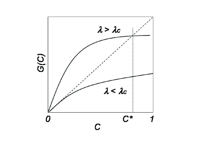
Figure 1: The functions $G(C)$, given in Eq. (4.2), with two different values of $\lambda$. When $\lambda>\lambda_{c}$, there will be a positive, stable node corresponding to an endemic steady state with a sustained infection.

4.1 Linear analysis of steady states

One can linearize equation (3.7) near its steady states and obtain

$$\frac{d\vec{y}}{dt}=B\vec{y},$$ (4.6)

in which the linear community matrix $B$ has elements

$$B_{kl}(\vec{y^{*}})=\frac{\lambda kl(D_{k}-y_{k}^{*})}{\langle k\rangle}-\delta_{kl}\left(\lambda k\frac{\sum_{j=1}^{K}jy_{j}^{*}}{\langle k\rangle}+1\right).$$ (4.7)

At the non-trivial, internal steady state, one can further obtain the complete eigenvalues of $B$:

$$\Lambda_{1}=-\lambda C^{*},\ \ \Lambda_{k}=-\lambda kC^{*}-1;\ \ 2\leq k\leq K.$$ (4.8)

Therefore this steady state is a locally stable node. This means that there is no any indication of oscillatory behavior, at this deterministic level, near the steady state.

At the steady state for extinction: $\vec{y^{*}}=\vec{0}$, we have $B_{kl}=\lambda klD_{k}/\langle k\rangle-\delta_{kl}$ from (4.7), which yields the eigenvalues

$$\Lambda_{1}=\lambda\frac{\sum k^{2}D_{k}}{\langle k\rangle}-1,\ \ \Lambda_{i}=-1;\ \ 2\leq i\leq K.$$ (4.9)

The eigenvector corresponding to the first eigenvalue $\Lambda_{1}$ is

$$\left\{1,\underbrace{\cdots,\ \frac{iD_{i}}{D_{1}\langle k^{2}\rangle}\left(\sum_{k\neq i}^{K}k^{2}D_{k}+D_{i}\right)>0,\cdots}_{i=2,3,\cdots,K}\right\}.$$ (4.10)

In the neighborhood of $\vec{0}$, this eigenvector locates within the first quadrant. It is stable when $\lambda\langle k^{2}\rangle/\langle k\rangle<1$, and unstable when $\lambda\langle k^{2}\rangle/\langle k\rangle>1$.

5 Non-equilibrium fluctuations near the positive stable node

We now turn our attention to stochastic dynamics near the stable internal steady state $\vec{y}=\vec{y^{*}}$. Note that we have shown through the above linear analysis that $\vec{y^{*}}$ is a node, with all eigenvalues being real. To consider stochastic fluctuations, we consider Eq. (3.8). Substituting the deterministic steady state solution into Eq. (3.8), it is reduced to a time-homogeneous Fokker-Planck equation defined on the entire $\mathbb{R}^{K}$

$$\frac{\partial\Pi(\vec{\xi},t)}{\partial t}=\nabla\cdot\left(\frac{A}{2}\nabla\Pi(\vec{\xi},t)-B\vec{\xi}\ \Pi(\vec{\xi},t)\right),$$ (5.1)

whose stationary solution is called Ornstein-Uhlenbeck (OU) process.

For the trivial stable node, the corresponding Fokker-Planck equation is only defined on the first quadrant. This leads to a singular diffusion equation, which is outside the scope of the present paper and will be the subject of a separated study.

The constant drift matrix in Eq. (5.1) is precisely the community matrix $B$ in Eq. (4.6). The diffusion tensor is a diagonal matrix $A_{kk}(\vec{y^{*}})=2y_{k}^{*}$ since we have the useful relationship $\frac{\lambda k}{\langle k\rangle}(D_{k}-y_{k})\sum jy_{j}^{*}=y_{k}^{*}$ from Eq. (3.7). The stochastic trajectories of OU process defined by Eq. (5.1) follows a linear stochastic differential equation:

$$\frac{d\vec{\xi}}{dt}=B\vec{\xi}(t)+\Gamma\vec{\zeta}(t),$$ (5.2)

where $\Gamma\Gamma^{T}=A$, $\vec{\zeta}(t)$ is a Gaussian white noise with $E[\vec{\zeta}(t)\vec{\zeta}^{T}(t^{\prime})]=\delta(t-t^{\prime})I$, and $I$ is the identity matrix.

If one sets the initial condition

$$\Pi(\xi,0)=\prod_{i=1}^{K}\delta\left(\xi_{i}-\xi_{i}^{o}\right),$$ (5.3)

Then the fundamental solution, i.e., Green’s function, to Eq. (5.1) is a multivariate Gaussian distribution [39, 40].

$$\Pi(\vec{\xi},t)=\Pi_{0}\exp\left\{-\frac{1}{2}\left(\vec{\xi}-\vec{\mu}(t)\right)^{T}\Xi(t)^{-1}\left(\vec{\xi}-\vec{\mu}(t)\right)\right\},$$ (5.4)

where $\Pi_{0}$ is a normalization factor. The first and second order moments satisfy [22]:

$$\frac{d\mu_{k}(t)}{dt}=\sum_{j}B_{kj}\mu_{k},\ \ \ \frac{d\Xi(t)}{dt}=B\Xi+\Xi B^{T}+A.$$ (5.5)

The solutions to Eq. (5.5) are:

$$\vec{\mu}(t)=e^{tB}\vec{\xi}_{0},\ \ \ \Xi(t)=\int_{0}^{t}e^{(t-t^{\prime})B}Ae^{(t-t^{\prime})B^{T}}dt^{\prime}.$$ (5.6)

Since the eigenvalues of $B$ are all negative, we have ${\langle\vec{\xi}\rangle}(\infty)=\vec{0}$ and $\Xi(t)$ approaches to a $\Xi^{s}$ as the solution to Eq. (5.7):

$$B\Xi^{s}+\Xi^{s}B^{T}=-A.$$ (5.7)

Equation (5.7) is analogue to the well-known Einstein’s fluctuation-dissipation relation, in which $A$ is the covariance of the fluctuating white noise, $B$ is the dissipative linear relaxation rates, and $\Xi^{s}$ is the equilibrium covariance. In thermal physics, $\Xi^{s}$ is proportional to $k_{B}T$.

Very interestingly, we note that $A^{-1}B$ is not symmetric. This implies the stationary process has certain breaking symmetry with respect to time reversal [40]. In physics, there is a refined distinction between an equilibrium and a non-equilibrium steady state. Such a distinction is not widely appreciated in dynamical descriptions of biological populations in terms of differential equations in which fixed point, steady state, and equilibrium are all synonymous.

According to the method previously developed in physics [3, 40, 41], there exists a stationary circular current density

$$\vec{j}^{(c)}=(\Phi\vec{\xi})\Pi^{s}(\vec{\xi}),$$ (5.8)

in which $\Phi$ is a $K\times K$ matrix with zero trace and $\vec{j}^{(c)}$ is a divergence free vector field $\nabla\cdot\vec{j}^{(c)}=0$. The linear force $B\vec{\xi}$ near the steady state, then, can be decomposed into two orthogonal parts

$$B=-\frac{1}{2}A\Xi^{-1}+\Phi.$$ (5.9)

In Eq. (5.9), the first term $-\frac{1}{2}A\Xi^{-1}\vec{\xi}$ is a conservative force with a potential function $U(\vec{\xi})=$ $\frac{1}{2}\vec{\xi}^{T}\left(\Xi^{s}\right)^{-1}\vec{\xi}$. It generates a motion towards the origin. In another words, it represents a stability landscape $\textsl{U}(\vec{\xi})$. The second term $\Phi\vec{\xi}$ generates a stationary circular motion on the level set of U. To see this, we observe the orthogonality

$$\vec{j}^{(c)}\perp\nabla\Pi(\vec{\xi})$$ (5.10)

due to $\vec{\xi}^{T}\Xi^{-1}\Phi\vec{\xi}=0$. The stationary probability distribution does not change along the direction of $\vec{j}^{(c)}$. The maintenance of the stationary distribution comes from two parts: one is the detailed along the gradient of $U(\vec{\xi})$, and another is circular along its level curve.

For heterogeneous SIS with two subgroups, i.e., $K=2$ and $k=1,\ 2$, the matrix $B$ from Eq. (4.7) is

$$B=\left(\begin{array}[]{cc}\frac{\lambda(D_{1}-2y_{1}^{*}-2y_{2}^{*})}{D_{1}+2D_{2}}-1&\frac{2\lambda(D_{1}-y_{1}^{*})}{D_{1}+2D_{2}}\\[5.0pt] \frac{2\lambda(D_{2}-y_{2}^{*})}{D_{1}+2D_{2}}&\frac{2\lambda(2D_{2}-y_{1}^{*}-4y_{2}^{*})}{D_{1}+2D_{2}}-1\end{array}\right),$$ (5.11)

and matrix

$$A=\left(\begin{array}[]{cc}2y_{1}^{*}&0\\ 0&2y_{2}^{*}\end{array}\right),$$ (5.12)

in which $y_{2}^{*}\in(0,D_{2}]$ is a root of

$$4\left(y_{2}^{*}\right)^{2}-\left(2D_{1}+12D_{2}-\frac{\langle k\rangle}{\lambda}\right)y_{2}^{*}+2D_{2}\left(D_{1}+4D_{2}-\frac{\langle k\rangle}{\lambda}\right)=0,$$ (5.13)

and

$$y_{1}^{*}=\frac{\langle k\rangle y_{2}^{*}}{2\lambda(D_{2}-y_{2}^{*})}-2y_{2}^{*}.$$ (5.14)

Therefore, with parameters $\lambda=1$ and $D_{1}=D_{2}=\frac{1}{2}$, thus $\langle k\rangle=1.5$, the matrix

$$\Phi=\left(\begin{array}[]{cc}-0.0644&0.1204\\ -0.1903&0.0644\end{array}\right).$$ (5.15)

The eigenvalues of this $\Phi$ is pair of pure imaginary numbers $\pm 0.137i$. This reflects an intrinsic frequency of the dynamics. Fig. 2A shows how the frequency changes with $\langle k\rangle$ for several different values of $\lambda$. For heterogeneous populations with two subgroups $N_{1}$ and $N_{2}$, the maximal effect of heterogeneity has to be $\langle k\rangle$ between 1 and 2; where the imaginary eigenvalues of $\Phi$ is also the largest.

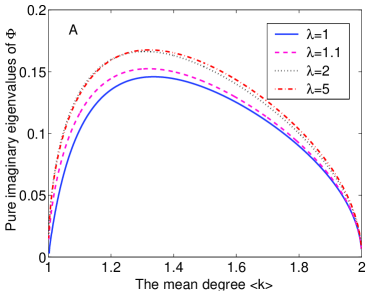
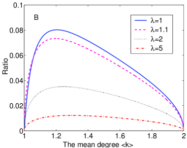
Figure 2: (A) For $K=2$, the intrinsic frequence, i.e., the pure imaginary eigenvalues of $\Phi$, as a function of $\langle k\rangle$ and $\lambda$. $\langle k\rangle$ changes from 1.999 to 1.001 due to $D_{1}$ changes from $1/1000$ to $999/1000$ , and the corresponding $D_{2}=1-D_{1}$ changes from $999/1000$ to $1/1000$. (B): the IR (imaginary-to-real) ratio, the ratio of the imaginary eigenvalues of $\Phi$ to the sums of two real eigenvalues of matrix $B$, as a function of $\langle k\rangle$ and $\lambda$. Note the critical $\lambda_{c}=1$ here; hence when $\lambda<1$ the endemic steady state disappears.

One of the widely used technique to capture and characterize oscillatory dynamics is the method of power spectrum [30]. For a strong oscillatory motion with noise, its power spectrum exhibits an off-zero peak at the intrinsic frequency. By “strong”, we mean the intrinsic frequency has to be significantly greater than the relaxation rate of the stochastic dynamics. [42] has shown that the ratio of imaginary part to real part of an eigenvalue has to be at least greater than $\frac{1}{\sqrt{3}}=0.577$. Fig. 2B shows the ratio between the intrinsic frequency, given by the imaginary eigenvalue of $\Phi$, and the relaxation rate, given by the eigenvalues of the community matrix $B$. This explains why one does not observe an off-zero peak in the power spectra of the simulated dynamics (data not shown).

6 Intrinsic circular dynamics in multi-dimensional birth-death processes

We now address a crucial question unanswered in Sec. 5: Whether the novel circular dynamics near the endemic steady state, shown by the OU approximation, is a consequence of the population-size expansion approximation, or is it a general result for the finite population birth-death process. The answer is affirmative. To illustrate this, we shall again consider the special case of $K=2$ and analyze the planar system in some detail. The same methods and results can easily be generalized to any $K>2$, but the algebra will be more cumbersome.

First, we need to address the issue of long-time behavior of the original birth-death process. In Sec. 4 we have shown that when $\lambda>\lambda_{c}$, the deterministic dynamics has a stable internal node representing an endemic steady state, while the extinction state $y_{i}=0$ $(1\leq i\leq K)$ is unstable. On the other hand, it had been shown in Sec. 2 that the infinite long-time behavior of the original birth-death process is always extinction, even though it might take extremely long time. This disparity between the stable deterministic steady state and the stochastic long-time behavior indicates a separation of two different time scales: The time scale on which the infectious dynamics reaches a stationary pattern among different populations, and the time scale for extinction of the infectious population [36, 43, 44]. In the light of the time-scale separation, this is a well-understood subject in population dynamics. There are in fact two fundamentally different types of extinction: one that occurs as a consequence of nonlinear dynamic, and another that occurs as rare events that is impossible according to nonlinear dynamics [37].

To study the “long-time” dynamics in the pre-extinction phase, one of the methods of attack is quasi-stationary approximation [36, 37, 43]. Conceptually, we only consider the stationary probability distribution conditioned on the survival probability at time $t$. To carry out the computation, one can introduce a very tiny transition probability $\varepsilon\ll 1$ representing the process can “return from” the state $\vec{0}$. This approximation abolishes the absorbing state. Since the total number of states is finite for our original birth-death process and it is irreducible, an unique stationary distribution exits. Biologically, the $\varepsilon$ can be interpreted as an infinitesimal invasion by migration, or recurrence, of infectious individuals. The time evolution of probability in (2.4a) then becomes

$$\frac{d}{dt}P(\vec{0},t)=\sum_{k=1}^{K}J_{-}^{k}(\vec{0}+e_{k})P(\vec{0}+e_{k})-\varepsilon\delta(P(\vec{0},t)\in[1-\varepsilon,1]).$$ (6.1)

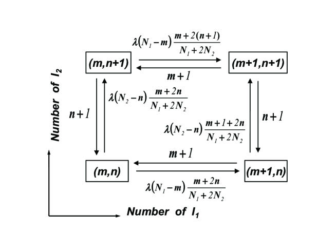
Figure 3: The “phase plane” for a two-dimensional birth-death process $\left(I_{1},I_{2}\right)$ where $I_{1}$ and $I_{2}$ take non-negative integers. All the possible transitions among four neighboring states are shown as the arrows and the corresponding rates are labeled by the transitions (i.e., Eq. (2.3)).

In the case of $K=2$, the probability transition rates in the planar system are illustrated in Fig. 3. Such a diagram is known as a master equation graph in stochastic chemical kinetics [45, 46]. It is useful tool in “visualizing” the dynamics of the master equation in Eq. (2.4), on a par with the phase portrait of planar nonlinear dynamics.

According to a key theorem in the theory of irreversible Markov chain, a sufficient and necessary condition for the existence of circular flux in the stationary process is the Kolmogorov cycle condition [29, 30]. In Fig. 3 the values for all the transition rates around a square cycle are given. Let $J_{+}^{(m,n)}$ denote the “clockwise” circular rate product

$$J_{+}^{(m,n)}=q_{(m,n)\rightarrow(m,n+1)}q_{(m,n+1)\rightarrow(m+1,n+1)}q_{(m+1,n+1)\rightarrow(m+1,n)}q_{(m+1,n)\rightarrow(m,n)},$$ (6.2)

in which the $q_{(m,n)\rightarrow(m,n+1)}$ is the transition rate from grid point $(m,n)$ to grid point $(m,n+1)$. Similarly $J_{-}^{(m,n)}$ is the “counterclockwise” rate product

$$J_{-}^{(m,n)}=q_{(m,n+1)\rightarrow(m,n)}q_{(m+1,n+1)\rightarrow(m,n+1)}q_{(m+1,n)\rightarrow(m+1,n+1)}q_{(m,n)\rightarrow(m+1,n)}.$$ (6.3)

Then the Kolmogorov cycle criterion $\theta$ for each little square cycle is:

$$\theta_{(m,n)}=\frac{J_{+}^{(m,n)}}{J_{-}^{(m,n)}}.$$ (6.4)

Substituting the values for the transition rates in Fig. 3, we have $\theta_{(m,n)}=\frac{m+2n+2}{m+2n+1}$, shown in Fig. 4. We note that $\theta_{(m,n)}$ is very close to $1$ for large $m$ or $n$. So generally the circular motion is weak. This explain why there is no circular motion in the deterministic dynamics of densities, when $N\rightarrow\infty$.

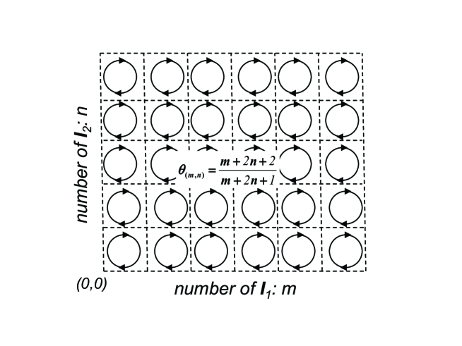
Figure 4: Stationary birth-death process can have a hidden circular dynamics, analogous to the vortex in a fluids [47]. The existence of stationary circulation can be determined by the Kolmogorov cycle number $\theta_{(m,n)}$. For our model with $K=2$, the $\theta_{(m,n)}=\frac{m+2n+2}{m+2n+1}$ and the circulation is always clockwise. For a larger, arbitrary closed circular path, the value of $\theta$ is the product of all the individual $\theta$’s within. A stationary Markov process is time-reversible if and only if all the $\theta$’s are 1. In mathematical statistics and in statistical physics, this is also known as detailed balance.

The $\theta_{(m,n)}$s in Fig. 4 can be heuristically understood as “vortex” in a vector field. They are the fundamental units of circular dynamics. For a larger closed circular path, its $\theta$ is simply the product of all the $\theta$’s within. The significance of the $\theta$ value lies in the theory of stationary, irreversible Markov processes. According to the cycle decomposition theorem for irreversible Markov processes [29], the $\theta_{(m,n)}$ is the ratio of numbers of occurrence, following the stationary, stochastic birth-death process, of the clockwise cycle $(m,n)\rightarrow(m,n+1)\rightarrow(m+1,n+1)\rightarrow(m+1,n)\rightarrow(m,n)$ to that of the corresponding counter-clockwise cycle. A stationary process is time-reversible if and only if each and every cycle has $\theta=1$.

The Fig. 4 gives the insight that the infection dynamics is “moving clockwise” in the phase plane in its stationary state. We know that a one-dimensional stationary birth-death process is always time-reversible. Therefore, irreversibility in the present example comes from the heterogeneity in the infectious population. This is a novel dynamical behavior emerged in population with heterogeneous structures.

In order to see things more clearly, we carried out stochastic simulations for the stochastic process. Firstly we consider two subgroups with $k=1,\ 2$. Other parameters used are $N_{1}=50$, $N_{2}=50$ and the transmission rate $\lambda=1$. The initial conditions are chosen randomly. Fig. 5 shows the typical trajectories of the two infecting population sizes, $I_{1}$ and $I_{2}$. For comparison, the two thick lines are the solutions to the corresponding deterministic equations (3.7): $y_{1}(t)\times N$ and $y_{2}(t)\times N$, respectively.

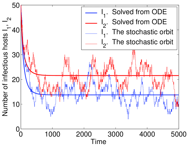
Figure 5: A typical stochastic realization of the SIS model. Here we considered two subgroups with $k=1,2$. The parameters used in simulation are $N_{1}=50$, $N_{2}=50$ (thus $\langle k\rangle=1.5$), and the transmission rate $\lambda=1$. The simulation is carried out according to Gillespie’s algorithm [48]. The thickened lines are orbits of the deterministic equations (3.7) with same $\lambda$ and $D_{1}=D_{2}=\frac{1}{2}$.

7 Conclusion and discussion

This paper has two intertwined threads. First, it reports a novel observation that for an SIS epidemic dynamics in a finite population with heterogeneous subgroups, there is an emergent inherent frequency, even though the corresponding deterministic nonlinear dynamics for infinite population shows no indication whatsoever. This result provides new insight to the understanding of fluctuations in epidemiological data.

Since the phenomenon is at the juncture between dynamics in terms of systems of deterministic ordinary differential equations (ODEs) and in terms of stochastic birth-death processes, the relation between these two types of mathematical models is rigorously investigated. We want to emphasize that in our approach, the nonlinear dynamics is an emergent, collective phenomenon of the stochastic population dynamics. The second thread of the paper, therefore, is to advance a systematic approach to nonlinear population dynamics based on individual’s behavior with uncertainties, which can be represented in terms of probability distributions. From this starting point, the traditionally employed ODEs can be more explicitly justified as the limiting behavior of infinitely large population for a nonlinear stochastic dynamics, called Delbrück-Gillespie process in cellular biochemistry [3, 46]. Furthermore, a Gaussian like stochastic process can also be derived to account for the population fluctuations in the large, but finite, population.

Indeed, on the level of individuals, epidemic processes are essentially stochastic, and the heterogeneity are inevitable. In the present study, we distinguish the stochastic, but statistically identical behavior (i.e., within each subgroup) from statistically non-identical behavior (i.e., between different subgroups). We show a more careful model building based “mechanisms” of the infection, though still quite crude, nevertheless can provide further insights into the dynamics on the population level.

One might wonder why the circular dynamics disappears in deterministic system. The reason lies in the equality $\theta_{(m,n)}=\frac{m+2n+2}{m+2n+1}$. As we have shown, the ODE dynamics equations are obtained from stochastic processes via the Law of Large Numbers, which is in order of $N^{-1}$, where $N$ is the total number of individuals in the population. In the limit of $N\rightarrow\infty$, $\theta_{(m,n)}\rightarrow 1$.

In summary, we proposed a microscopic, statistically heterogeneous contact process for individual-based epidemiological modeling. The fundamental stochastic events are the instantaneous “contacts” between two individuals and the recovery of an infectious individual. Within an infinitesimal time interval, these events are sequential and independent. The stochastic process is a Poisson flow. We applied this approach to two-state SIS dynamics. Following the method of $\Omega$ expansion, we obtained a system of deterministic ODEs for the densities for a large population, as well as a linear diffusion system near the stable steady state.

There are two time scales in the dynamics of SIS epidemics. Compared with the time in which the infection reaches a “stationary pattern” among the subgroups, the time for ultimate extinction is very long when $\lambda>\lambda_{c}$ [37]. We used the method of quasi-stationary approximation to study the long-time behavior on the “short time scale”.

Another assumption adopted here is the mass action law which requires well mixing. In population dynamic term, it is assumed that individuals are moving rapidly within a relatively small, highly “fluid” community. In a large spatial scales, the contacts and spatial movements involve geographic factors; then a spatial model is required. In the applications of epidemic dynamic models to “virus infection” on the World Wide Web, however, this restriction is hardly there.

8 Acknowledgements

JZW acknowledges support from China Postdoctoral Science Foundation (Special Grade No. 201003021), Beijing Municipal Government Fund for Talents (2011, No. D005003000009), and the NSFC (No. 11001004). HQ thanks T. C. Reluga for helpful comments.

References

- [1] Murray J. D., 2007. Mathematical Biology: I. An Introduction. 3rd ed., Spinger, New York.
- [2] Kot M., 2001. Elements of Mathematical Ecology. Cambridge Univ. Press, UK.
- [3] Qian H., 2011. Nonlinear stochastic dynamics of mesoscopic homogeneous biochemical reactions systems - An analytical theory. Nonlinearity, 24. R19–R49.
- [4] Lajmanovich A. and Yorke J. A., 1976. A deterministic model for gonorrhea in a nonhomogeneous population. Math. Biosci., 28. 221–236.
- [5] Woolhouse M. E. J., et. al., 1997. Heterogeneities in the trasmission of infectious agents: Implications for the design of control programs. Proc. Natl. Acad. Sci. U.S.A., 94. 338–342.
- [6] Jacquez J. A., Simon C. and Koopman. J. S., 1995. Core groups and for subgroups in heterogenous SIS and SI models. In Epidemic Models: Their Structure and Relation to Data, D. Mollison ed., Cambridge Univ. Press, UK.
- [7] Liljeros F., Edling C. R., Amaral L. A. N., Stanley H. E., and Abers Y., 2001. The web of human sexual contacts. Nature, 411. 907.
- [8] Schneeberger A., et. al., 2004. Scale-free networks and sexually transmitted diseases: A description of Observed patterns of sexual contacts in Britain and Zimbabwe. Sexually Transmitted Diseases, 31. 380.
- [9] Barabási A. L., R. Albert, and H. Jeong, 2000. Scale-free characteristics of random networks: the topology of the world wide web. Physica A, 281. 69-77.
- [10] Pastor-Satorras R., Vázquez A., and Vespignani A., 2001. Dynamical and correlation properties of the internet. Phys. Rev. Lett., 87. 258701.
- [11] Colizza V., Barrat A., Barthelemy M., and Vespignani A., 2006. The role of the airline transportation network in the prediction and predictability of global epidemics. Proc. Natl. Acad. Sci. U.S.A., 103. 2015-2020.
- [12] Anderson R. M. and May R. M., 1991. Infectious Diseases of Humans: Dynamics and control. Oxford Univ. Press, Oxford.
- [13] May R. M., and Lloyd A. L., 2001. Infection dynamics on scale-free networks. Phys. Rev. E, 64. 066112.
- [14] Pastor-Satorras R., and Vespignani A., 2001. Epidemic spreading in scale-free networks. Phys. Rev. Lett, 86. 3200.
- [15] Wang J.-Z., Liu Z., and Xu J., 2007. Epidemic spreading on uncorrelated heterogenous networks with non-uniform transmission. Physica A, 382. 715–721.
- [16] Nåsell I., 2003. Moment closure and the stochastic logistic model. Theor. Popul. Biol., 63. 159-168.
- [17] Dangerfield C. E., et.al., 2009. Integrating stochasticity and network structure into epidemic model. J. R. Soc. Interface, 6. 761-774.
- [18] Bauch C. and Rand D. A., 2000. A moment closure model for sexuallytransmited disease transmission through a concurrent partnership network. Proc. R. Soc. Lond. B, 267. 2019-2027.
- [19] Anderson H., Britton T., 2000. Stochastic Epidemic Models and Their Statistical Analysis. Springer.
- [20] Hufnagel L., Brockmann D., and Geisel T., 2004. Forecast and control of epidemics in a globalized world. Proc. Natl. Acad. Sci. U.S.A., 101. 15124-15129.
- [21] Durrett R. and Levin S., 1994. The importance of being discrete. Theor. Popul. Biol., 46. 363-394.
- [22] van Kampen N. G., 2010. Stochastic Processes in Physics and Chemistry, 3rd ed., Elsevier, Amsterdam.
- [23] Bjornstad O. N. and Grenfell B. T., 2001. Noisy clockwork: Time series Analysis of population fluctuations in animals. Science, 293. 638.
- [24] Hethcote H. W. and van den Driessche P., 1991. Some epidemiological models with ninlinear incidence. J. Math. Biol., 29. 271.
- [25] Dushoff J., et.al., 2004. Dynamical resonance can account for seasonality of influenza epidemics. Proc. Natl. Acad. Sci. U.S.A., 101. 16915.
- [26] Alonso D., et. al., 2007. Stochastic amplification in epidemics. J. R. Soc. Interface, 4. 575-582.
- [27] Simones M., et. al., 2007. Stochastic fluctuations in epidemics on networks. J. R. Soc. Interface, 5. 555-566.
- [28] Qian H., Saffarian S. and Elson E.L., 2002. Concentration fluctuations in a mesoscopic oscillating chemical reaction system. Proc. Natl. Acad. Sci. U.S.A., 99. 10376-10381.
- [29] Jiang D.-Q., Qian M. and Qian M.-P., 2004. Mathematical Theory of Nonequilibrium Steady States On the frontier of probability and dynamical systems. LNM Vol. 1833. Springer-Verlag, Berlin.
- [30] Zhang X.-J., Qian H. and Qian M., 2012. Stochastic theory of nonequilibrium steady states and its applications (Part I). Phys. Rep., 510. 1–86.
- [31] Ge H., Qian M. and Qian H., 2012. Stochastic theory of nonequilibrium steady states (Part II): Applications in chemical biophysics. Phys. Rep., 510. 87–118.
- [32] Wolynes P. G., 1989. Chemical reaction dynamics in complex molecular systems. In Complex Systems: Santa Fe Inst. Studies in the Sci. of Complexity, D. Stein ed., Addision-Wesley Longman Pub., New York, pp. 355–387.
- [33] Bharucha-Reid A. T., 1960. Elements of the Theory of Markov Processes and Their Applications. McGraw-Hill, New York.
- [34] Ethier S. N. and Kurtz T. G., 1986. Markov Processes: Characterization and Convergence. John Wiley & Sons, New York.
- [35] Lotka A. J., 1910. Contribution to the theory of periodic reaction. J. Phys. Chem., 14. 271–274.
- [36] Nåsell I., 2001. Extinction and quasi-stationarity in the Verhulst logistic model. J. Theor. Biol., 211. 11-27.
- [37] Zhou D. and Qian H., 2011. Fixation, transient landscape and diffusion’s dilemma in stochastic evolutionary game dynamics. Phys. Rev. E. 84, 031907.
- [38] Gross T. and Kevrekidis I. G., 2008. Robust oscillations in SIS epidemics on adaptive networks: Coarse graining by automated moment closure. Eur. Phys. Lett. 82. 38004.
- [39] Fox R. F., 1978. Gaussian stochastic processes in physics. Phys. Rep., 48. 179-283.
- [40] Qian H., 2001. Mathematical formalism for isothermal linear irreversibility. Proc. Roy. Soc. Lond. A, 457. 1645-1655.
- [41] Kwon C.-L., Ao P. and Thouless D.J., 2005. Structure of stochastic dynamics near fixed points. Proc. Natl. Acad. Sci. U.S.A., 102. 13029–13033.
- [42] Qian H. and Qian M., 2000. Pumped biochemical reactions, nonequilibrium circulation, and stochastic resonance. Phys. Rev. Lett. 84. 2271–2274.
- [43] Vellela M., and Qian H., 2007. A quasistationary analysis of a stochastic chemical reaction: Keizer’s paradox. Bullet. Math. Biol., 69. 1727–1746.
- [44] Zhou D., Wu B. and Ge H., 2010. Evolutionary stability and quasi-stationary strategy in stochastic evolutionary game dynamics. J. Theor. Biol. 264. 874–881.
- [45] Beard D. A. and Qian H., 2008. Chemical Biophysics: Quantitative Analysis of Cellular Systems. Cambridge Texts in Biomed. Engr., Cambridge Univ. Press, London.
- [46] Qian H. and Bishop L. M., 2010. The chemical master equation approach to nonequilibrium steady-state of open biochemical systems: Linear single-molecule enzyme kinetics and nonlinear biochemical reaction networks. Internat. J. Mol. Sci., 11. 3472-3500.
- [47] Qian H., 1998. Vector field formalism and analysis for a class of Brownian ratchets. Phys. Rev. Lett., 81. 3063–3066.
- [48] Gillespie D. T., 1977. Exact stochastic simulation of coupled chemical reactions. J. Phys. Chem., 81. 2340-2361.