Supersymmetric mass spectra and the seesaw type-I scale

Abstract

We calculate supersymmetric mass spectra with cMSSM boundary conditions and a type-I seesaw mechanism added to explain current neutrino data. Using published, estimated errors on SUSY mass observables for a combined LHC+ILC analysis, we perform a theoretical $\chi^{2}$ analysis to identify parameter regions where pure cMSSM and cMSSM plus seesaw type-I might be distinguishable with LHC+ILC data. The most important observables are determined to be the (left) smuon and selectron masses and the splitting between them, respectively. Splitting in the (left) smuon and selectrons is tiny in most of cMSSM parameter space, but can be quite sizeable for large values of the seesaw scale, $m_{SS}$. Thus, for very roughly $m_{SS}\geq 10^{14}$ GeV hints for type-I seesaw might appear in SUSY mass measurements. Since our numerical results depend sensitively on forecasted error bars, we discuss in some detail the accuracies, which need to be achieved, before a realistic analysis searching for signs of type-I seesaw in SUSY spectra can be carried out.

I Introduction

The seesaw mechanism Minkowski:1977sc ; seesaw ; MohSen ; Schechter:1980gr ; Cheng:1980qt provides a rationale for the observed smallness of neutrino masses Fukuda:1998mi ; Ahmad:2002jz ; Eguchi:2002dm ; arXiv:0801.4589 ; Schwetz:2008er ; Nakamura:2010zzi . However, due to the large mass scales involved, no direct experimental test of “the seesaw” will ever be possible. Extending the standard model (SM) only by a seesaw mechanism does not even allow for indirect tests, since all possible new observables are suppressed by (some power of) the small neutrino masses.

The situation looks less bleak in the supersymmetric version of the seesaw. This is essentially so, because soft SUSY breaking parameters are susceptible to all particles and couplings which appear in the renormalization group equation (RGE) running. Thus, assuming some simplified boundary conditions at an high energy scale, the SUSY softs at the electro-weak scale contain indirect information about all particles and intermediate scales. Perhaps the best known application of this idea is the example of lepton flavour violation (LFV) in seesaw type-I with cMSSM boundary conditions, discussed already in Borzumati:1986qx . A plethora of papers on LFV, both for low-energy and for accelerator experiments, have been published since then (for an incomplete list see, for example, Hisano:1995nq ; Hisano:1995cp ; Ellis:2002fe ; Deppisch:2002vz ; Arganda:2005ji ; Antusch:2006vw ; Arganda:2007jw ; Hisano:1998wn ; Blair:2002pg ; Freitas:2005et ; Petcov:2003zb ; arXiv:0804.4072 ; 929607 ), most of them concentrating on seesaw type-I.

Seesaw type-I is defined as the exchange of fermionic singlets. At tree-level there is also the possibility to exchange (Y=2) scalar triplets Schechter:1980gr ; Cheng:1980qt , seesaw type-II, or exchange (Y=0) fermionic triplets, the so-called seesaw type-III Foot:1988aq ; Ma:1998dn . Common to all three seesaws is that for $m_{\nu}\sim\sqrt{\Delta m^{2}_{\textsc{A}}}\sim 0.05$ eV, where $\Delta m^{2}_{\textsc{A}}$ is the atmospheric neutrino mass splitting, and couplings of order ${\cal O}(1)$ the scale of the seesaw is estimated to be very roughly $m_{SS}\sim 10^{15}$ GeV. Much less work on SUSY seesaw type-II and type-III has been done than for type-I. For studies of LFV in SUSY seesaw type-II, see for example Rossi:2002zb ; arXiv:0806.3361 , for type-III arXiv:1010.6000 ; Biggio:2010me .

Apart from the appearance of LFV, adding a seesaw to the SM particle content also leads to changes in the absolute values of SUSY masses with respect to cMSSM expectations, at least in principle. Type-II and type-III seesaw add superfields, which are charged under the SM group. Thus, the running of the gauge couplings is affected, leading to potentially large changes in SUSY spectra at the EW scale. In Buckley:2006nv it was pointed out, that for type-II and type-III seesaw certain combinations of soft SUSY breaking parameters are at 1-loop order nearly constant over large parts of cMSSM parameters space, but show a logarithmic dependence on $m_{SS}$. This was studied in more detail, including 2-loop effects in the RGEs, for type-II in arXiv:0806.3361 and for type-III in arXiv:1010.6000 . Using forecasted errors on SUSY masses, obtained from full simulations Weiglein:2004hn ; AguilarSaavedra:2005pw , the work Hirsch:2011cw calculated the error with which the seesaw (type-II and -III) scale might be determined from LHC and future ILC AguilarSaavedra:2001rg measurements. Interestingly, Hirsch:2011cw concluded that, assuming cMSSM boundary conditions, ILC accuracies on SUSY masses should be sufficient to find at least some hints for a type-II/type-III seesaw, for practically all relevant values of the seesaw scale.

Seesaw type-I, on the other hand, adds only singlets. Changes in SUSY spectra are expected to be much smaller and, therefore, much harder to detect. Certainly because of this simple reasoning much fewer papers have studied this facet of the type-I SUSY seesaw so far. Running slepton masses with a type-I seesaw have been discussed qualitatively in Blair:2002pg ; Freitas:2005et ; Deppisch:2007xu ; Kadota:2009sf . In Abada:2010kj it was discussed that in cMSSM extended by a type-I seesaw, splitting in the slepton sector can be considerably larger than in the pure cMSSM. This is interesting, since very small mass splittings in the smuon/selectron sector might be measurable at the LHC, if sleptons are on-shell in the decay chain $\chi^{0}_{2}\to l^{\pm}{\tilde{l}}^{\mp}\to l^{\pm}l^{\mp}\chi^{0}_{1}$ Allanach:2008ib .

In this paper, we calculate SUSY spectra with cMSSM boundary conditions and a seesaw type-I. We add three generations of right-handed neutrinos and take special care that observed neutrino masses and mixing angles are always correctly fitted. We then follow the procedure of Hirsch:2011cw . Using predicted error bars on SUSY mass measurements for a combined LHC+ILC analysis, we construct fake “experimental” observables and use a $\chi^{2}$-analysis to estimate errors on the parameters of our model, most notably the seesaw scale. We identify regions in parameter space, where hints for a type-I seesaw might show up at the ILC/LHC and discuss quantitatively the accuracy which need to be achieved, before a realistic analysis searching for signs of type-I seesaw in SUSY spectra can be carried out.

The rest of this paper is organized as follows. In the next section we define the supersymetric seesaw type-I model, fix the notation and define the cMSSM. In section III we present our results. After a short discussion of the procedures and observables in section III.1, we show a simplified analysis, which allows to identify the most important observables and discuss their relevant errors in section III.2. Section III.3 then shows our full numerical results. We then close with a short summary and discussion in section IV.

II Setup

II.1 Supersymmetric seesaw type-I

In the case of seesaw type-I one postulates very heavy right-handed neutrinos with the following superpotential below the GUT scale, $M_{G}$:

$$W_{I} = W_{MSSM}+W_{\nu}.$$ (1)

Here $W_{MSSM}$ is the usual MSSM part and

$$W_{\nu} = {\widehat{N}}^{c}_{i}Y^{\nu}_{ij}{\widehat{L}}_{j}\cdot{\widehat{H}}_{u}+\frac{1}{2}{\widehat{N}}^{c}_{i}M_{R,ii}{\widehat{N}}^{c}_{i}\thickspace.$$ (2)

We have written eq. (1) in the basis where $M_{R}$ and the charged lepton Yukawas are diagonal. In the seesaw one can always choose this basis without loss of generality. For the neutrino mass matrix, upon integrating out the heavy Majorana fields, one obtains the well-known seesaw formula

$$m_{\nu}=-\frac{v^{2}_{u}}{2}Y^{\nu,T}M^{-1}_{R}Y^{\nu},$$ (3)

valid up to order ${\cal O}(m_{D}/M_{R})$, $m_{D}=\frac{v_{u}}{\sqrt{2}}Y^{\nu}$. Being complex symmetric, the light Majorana neutrino mass matrix in eq. (3), is diagonalized by a unitary $3\times 3$ matrix $U$ Schechter:1980gr

$${\hat{m}_{\nu}}=U^{T}\cdot m_{\nu}\cdot U\ .$$ (4)

Inverting the seesaw equation, eq. (3), allows to express $Y^{\nu}$ as Casas:2001sr

$$Y^{\nu}=\sqrt{2}\frac{i}{v_{u}}\sqrt{\hat{M}_{R}}\cdot R\cdot\sqrt{{\hat{m}_{\nu}}}\cdot U^{\dagger},$$ (5)

where the $\hat{m}_{\nu}$ and $\hat{M}_{R}$ are diagonal matrices containing the corresponding eigenvalues. $R$ is in general a complex orthogonal matrix. Note that, in the special case $R={\bf 1}$, $Y^{\nu}$ contains only “diagonal” products $\sqrt{M_{i}m_{i}}$. For $U$ we will use the standard form

$$U=\left(\begin{array}[]{ccc}c_{12}c_{13}&s_{12}c_{13}&s_{13}e^{-i\delta}\\ -s_{12}c_{23}-c_{12}s_{23}s_{13}e^{i\delta}&c_{12}c_{23}-s_{12}s_{23}s_{13}e^{i\delta}&s_{23}c_{13}\\ s_{12}s_{23}-c_{12}c_{23}s_{13}e^{i\delta}&-c_{12}s_{23}-s_{12}c_{23}s_{13}e^{i\delta}&c_{23}c_{13}\end{array}\right)\times\left(\begin{array}[]{ccc}e^{i\alpha_{1}/2}&0&0\\ 0&e^{i\alpha_{2}/2}&0\\ 0&0&1\end{array}\right)$$ (12)

with $c_{ij}=\cos\theta_{ij}$ and $s_{ij}=\sin\theta_{ij}$. The angles $\theta_{12}$, $\theta_{13}$ and $\theta_{23}$ are the solar neutrino angle, the reactor angle and the atmospheric neutrino mixing angle, respectively. $\delta$ is the Dirac phase and $\alpha_{i}$ are Majorana phases. Since $U$ can be determined experimentally only up to an irrelevant overall phase, one can find different parameterizations of the Majorana phases in the literature.

Eq. (3) contains 9 a priori unknown parameters, eq. (5) contains 18. The additional 9 unknowns encode the information about the high scale parameters, the three eigenvalues of $M_{R}$ and the 3 moduli and 3 phases of $R$.

II.2 cMSSM, type-I seesaw and RGEs

The cMSSM is defined at the GUT-scale by: a common gaugino mass $M_{1/2}$, a common scalar mass $m_{0}$ and the trilinear coupling $A_{0}$, which gets multiplied by the corresponding Yukawa couplings to obtain the trilinear couplings in the soft SUSY breaking Lagrangian. In addition, at the electro-weak scale, $\tan\beta=v_{u}/v_{d}$ is fixed. Here, as usual, $v_{d}$ and $v_{u}$ are the vacuum expectation values (vevs) of the neutral component of $H_{d}$ and $H_{u}$, respectively. Finally, the sign of the $\mu$ parameter has to be chosen.

Two-loop RGEs for general supersymmetric models have been given in Martin:1993zk . In our numerical calculations we use SPheno3.1.5 Porod:2003um ; Porod:2011nf , which solves the RGEs at 2-loop, including right-handed neutrinos. It is, however, useful for a qualitative understanding, to consider first the simple solutions to the RGE for the slepton mass parameters found in the leading log approximation Hisano:1995cp ; Hisano:1998wn , given by

$$(\Delta M_{\tilde{L}}^{2})_{ij} = -\frac{1}{8\pi^{2}}(3m_{0}^{2}+A_{0}^{2})(Y^{\nu,\dagger}LY^{\nu})_{ij}$$ (13)

$$(\Delta A_{l})_{ij} = -\frac{3}{8\pi^{2}}A_{0}Y_{l_{i}}(Y^{\nu,\dagger}LY^{\nu})_{ij}$$

$$(\Delta M_{\tilde{E}}^{2})_{ij} = 0,$$

where only the parts proportional to the neutrino Yukawa couplings have been written. The factor $L$ is defined as

$$L_{kl}=\log\Big{(}\frac{M_{G}}{M_{k}}\Big{)}\delta_{kl}.$$ (14)

Eq. (13) shows that, within the type-I seesaw mechanism, the right slepton parameters do not run in the leading-log approximation. Thus, LFV is restricted to the sector of left-sleptons in practice, apart from left-right mixing effects which could show up in the scalar tau sector. Also note that for the trilinear parameters running is suppressed by charged lepton masses.

It is important that the slepton mass-squareds involve a different combination of neutrino Yukawas and right-handed neutrino masses than the left-handed neutrino masses of eq. (3). In fact, since $(Y^{\nu,\dagger}LY^{\nu})$ is a hermitian matrix, it obviously contains only nine free parameters Ellis:2002fe , the same number of unknowns as on the right-hand side of eq. (5), given that in principle all 3 light neutrino masses, 3 mixing angles and 3 CP phases are potentially measurable.

Apart from the slepton mass matrices, $Y^{\nu}$ also enters the RGEs for $m_{H_{u}}^{2}$ at 1-loop level. However, we have found that the masses of the Higgs bosons are not very sensitive to the values of $Y^{\nu}$, see also next section. We thus do not give approximate expressions for $m_{H_{u}}^{2}$. For all other soft SUSY parameters, $Y^{\nu}$ enters only at the 2-loop level. Thus, the largest effects of the SUSY type-I seesaw are expected to be found in the left slepton sector.

III Numerical results

III.1 Preliminaries

We use SPheno3.1.5 Porod:2003um ; Porod:2011nf to calculate all SUSY spectra and fit the neutrino data. Unless noted otherwise the fit to neutrino data is done for strict normal hierarchy (i.e. $m_{\nu_{1}}=0$), best-fit values for the atmospheric and solar mass squared splitting Schwetz:2008er and tri-bimaximal mixing angles hep-ph/0202074 . To reduce the number of free parameters in our fits, we assume right-handed neutrinos to be degenerate and $R$ to be the identity. The seesaw scale, called $m_{SS}$ below, is equal to the degenerate right-handed neutrino masses. We will comment on expected changes of our results, when any of these assumptions is dropped in the next subsections. Especially, recently there have been some indications for a non-zero reactor angle, both from the long-baseline experiment T2K arXiv:1111.0183 as well as from the first data in Double CHOOZ DC2011 . We will therefore comment also on non-zero values of $\theta_{13}=\theta_{R}$.

SPheno solves the RGEs at 2-loop level and calculates the SUSY masses at 1-loop order, except for the Higgs mass, where the most important 2-loop corrections have been implemented too. Theoretical errors in the calculation of the SUSY spectrum are thus expected to be much smaller than experimental errors at the LHC. However, since for the ILC one expects much smaller error bars, theory errors will become important at some point. We comment on theory errors in the discussion section.

Observables and their theoretically forecasted errors are taken from the tables (5.13) and (5.14) of Weiglein:2004hn and from AguilarSaavedra:2005pw . For the LHC we take into account the “edge variables”: $(m_{ll})^{edge}$, $(m_{lq})^{\text{edge}}_{\text{low}}$, $(m_{lq})^{\text{edge}}_{\text{high}}$, $(m_{llq})_{\rm edge}$ and $(m_{llq})_{\rm thresh}$ from the decay chain ${\tilde{q}}_{L}\to\chi^{0}_{2}q$ and $\chi^{0}_{2}\to l{\tilde{l}}\to ll\chi^{0}_{1}$ Bachacou:1999zb ; Allanach:2000kt ; Lester:2001zx . In addition, we consider $(m_{llb})_{thresh}$, $(m_{\tau^{+}\tau^{-}})$ (from decays involving the lighter stau) and the mass differences $\Delta_{{\tilde{g}}{\tilde{b}}_{i}}=m_{\tilde{g}}-m_{{\tilde{b}}_{i}}$, with $i=1,2$, $\Delta_{{\tilde{q}}_{R}\chi^{0}_{1}}=m_{{\tilde{q}}_{R}}-m_{\chi^{0}_{1}}$ and $\Delta_{{\tilde{l}}_{L}\chi^{0}_{1}}=m_{{\tilde{l}}_{L}}-m_{\chi^{0}_{1}}$. Since $m_{{\tilde{u}}_{R}}\simeq m_{{\tilde{d}}_{R}}\simeq m_{{\tilde{c}}_{R}}\simeq m_{{\tilde{s}}_{R}}$ applies for a large range of the parameter space LHC measurements will not be able to distinguish between the first two generation squarks. The combined errors for an LHC+ILC analysis, tables (5.14) of Weiglein:2004hn , are dominated by the ILC for all non-coloured sparticles, except the stau. For us it is essential that both, left and right sleptons are within reach of the ILC. Also the two lightest neutralinos and the lighter chargino measured at ILC are important. The errors in Weiglein:2004hn were calculated for relatively light SUSY spectra, thus we extrapolate them to our study points, see below, assuming constant relative errors on mass measurements. We will comment in some detail on the importance of this assumption below. Finally, we use the splitting in the selectron/smuon sector Allanach:2008ib as an observable:

$$\Delta(m_{\tilde{e}\tilde{\mu}})=\frac{m_{\tilde{e}}-m_{\tilde{\mu}}}{m_{\tilde{l}}^{mean}}.$$ (15)

Here, ${m_{\tilde{l}}^{mean}}=\frac{1}{2}(m_{\tilde{e}}+m_{\tilde{\mu}})$. The LHC can, in principle, measure this splitting from the edge variables for both, left and right sleptons, if the corresponding scalars are on-shell. In cMSSM type-I seesaw only the left sector has a significant splitting, we therefore suppress the index “L” for brevity. For this splitting Allanach:2008ib quote a “one sigma observability” of $\Delta(m_{\tilde{e}\tilde{\mu}})\sim 2.8$ $\permil$ for SPS1a. For comparison, the errors on the left selectron and smuon mass at the ILC for this point are quoted as $\Delta(m_{\tilde{e}})\simeq 1$ $\permil$ and $\Delta(m_{\tilde{\mu}})\simeq 2.5$ $\permil$, respectively Weiglein:2004hn .

The negative searches for SUSY by CMS arXiv:1109.2352 and ATLAS arXiv:1109.6572 define an excluded range in cMSSM parameter space, ruling out the lightest SPS study points, such as SPS1a’ AguilarSaavedra:2005pw or SPS3 Allanach:2002nj . For our numerical study we define a set of five points, all of which are chosen to lie outside the LHC excluded region, but have the lightest non-coloured SUSY particles within reach of a 1 TeV linear collider. The points are defined as follows:

$${\rm P}_{1} \rightarrow (m_{0}=120,M_{1/2}=600,A_{0}=0,\tan\beta=10)$$

$${\rm P}_{2} \rightarrow (m_{0}=120,M_{1/2}=600,A_{0}=300,\tan\beta=10)$$

$${\rm P}_{3} \rightarrow (m_{0}=120,M_{1/2}=600,A_{0}=-300,\tan\beta=10)$$ (16)

$${\rm P}_{4} \rightarrow (m_{0}=180,M_{1/2}=550,A_{0}=0,\tan\beta=10)$$

$${\rm P}_{5} \rightarrow (m_{0}=180,M_{1/2}=550,A_{0}=300,\tan\beta=10)$$

All points have $sgn(\mu)>0$, masses are in units of GeV. Points $P_{1}$-$P_{3}$ lie very close to the stau-coannihilation line. We have checked by an explicit calculation with MicrOmegas hep-ph/0405253 ; hep-ph/0607059 ; arXiv:0803.2360 ; arXiv:1004.1092 that the relic density of the neutralino agrees with the current best fit value of $\Omega_{CDM}h^{2}$ within the quoted error bars Nakamura:2010zzi for $P_{1}$. $P_{4}$ and $P_{5}$ have been chosen such that deviations from the pure cMSSM case are larger than in $P_{1}$-$P_{3}$, see eq.(13), i.e. to maximize the impact of the seesaw type-I on the spectra, see below.

III.2 Observables and seesaw scale

In this subsection we will first keep all parameters at some fixed values, varying only the seesaw scale. These calculations are certainly simple-minded, but also very fast compared to the full Monte Carlo parameter scans, discussed later. However, as will be shown in the in the next subsection, there is nearly no correlation between different input parameters. Thus, the simple calculation discussed here already gives a quite accurate description of the results of the more complicated minimization procedures of the “full” calculation. Especially, this calculation allows us to identify the most important observables and discuss their maximally acceptable errors for our analysis.

In fig. (1) we show

$$\sigma_{i}=\frac{m_{i}^{m_{SS}}-m_{i}^{cMSSM}}{m_{i}^{cMSSM}}\Big{/}\Delta(m_{i}),$$ (17)

where $\Delta(m_{i})$ is the expected relative experimental error for the mass of sparticle i at the ILC, as a function of $m_{SS}$. We remind the reader that we assume that $\Delta(m_{i})$ can be extrapolated to our study points. To the left results for $P_{1}$ and to the right for $P_{5}$. $m_{i}^{cMSSM}$ is the value of the mass calculated in the cMSSM limit and $m_{i}^{m_{SS}}$ the corresponding mass for a seesaw scale of $m_{SS}$. These latter values have always been calculated fitting the Yukawa matrix of the neutrinos at $m_{SS}$, such that the best fit values of solar and atmospheric neutrino mass differences are obtained and $m_{\nu_{1}}\equiv 0$ is maintained. As expected the departures from the cMSSM values then increase with increasing seesaw scale. Note that the lines stop at values of $m_{SS}\sim(2-3)\times 10^{15}$ GeV, since for larger values neutrino Yukawas, which are required to fit the neutrino data, are non-perturbative.

Significant departures with respect to the cMSSM values are found (with decreasing importance) for the following observables: left smuon mass, left selectron mass, mass of $\chi^{0}_{1}$, $m_{h^{0}}$ and $\chi^{+}_{1}$. We have checked that all other observables have much milder dependences on $m_{SS}$, as expected. The smuon mass is more important than the selectron mass, despite the latter having a smaller predicted error, due to our choice of degnerate right-handed neutrinos in the fits. With this assumption the running of the smuon mass has contributions from Yukawas responsible for both, atmospheric and solar scale, while the selectron has contributions from the Yukawas of the solar scale only. The change in $\chi^{0}_{1}$ and $\chi^{+}_{1}$ masses are small in absolute scale, but it is expected that ILC will measure these masses with very high accuracy. Also $m_{h^{0}}$ shows some mild dependence on $m_{SS}$, but on a scale of an expected experimental error of $50$ MeV AguilarSaavedra:2005pw , i.e. much smaller than our current theoretical error, see below.

As the figure shows deviations from cMSSM expectations of the order of several standard deviations are reached for left smuon and selectron for values of $m_{SS}$ above $10^{14}$ GeV. Comparing the results for $P_{1}$ (left) with those for $P_{5}$ (right) it is confirmed that $P_{5}$ shows much larger deviations from cMSSM. We have checked that results for the other points $P_{2}$-$P_{4}$ fall in between the extremes of $P_{1}$ and $P_{5}$. Lines for $P_{2}$ and $P_{3}$ are nearly indistinguishable in such a plot, apart from some minor difference in the Higgs mass.

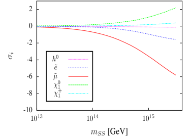
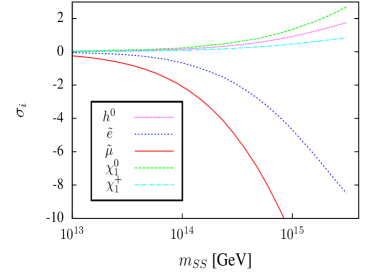
Figure 1: Calculated deviations of masses from their nominal cMSSM values as function of $m_{SS}$ for the most important masses. To the left $P_{1}$, to the right $P_{5}$.

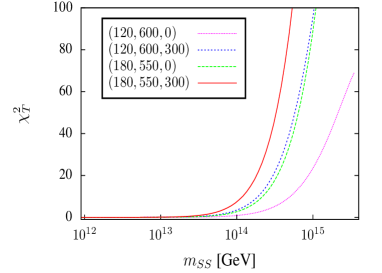
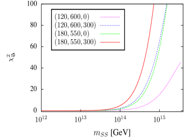
Figure 2: Calculated $\chi^{2}$ as function of $m_{SS}$ for 4 different cMSSM points. To the left: Total $\chi^{2}$ including all observables, to the right total $\chi^{2}_{\Delta\!\!\!\!\backslash}$, i.e. $\chi_{T}$ without the mass splitting in the (left) smuon-selectron sector. Values quoted in the plots correspond to ($m_{0},M_{1/2},A_{0}$). In all points shown we choose $\tan\beta=10$ and $\mu>0$.

In fig. (2) we show the calculated $\chi^{2}$ as a function of $m_{SS}$ for 4 different cMSSM points. Here, $\chi^{2}$ is calculated with respect to cMSSM expectations. To the left we show $\chi^{2}_{T}$ including all observables, to the right $\chi^{2}_{T}$ without the mass splitting in the (left) smuon-selectron sector. The figure demonstrates again that $P_{1}$ ($P_{5}$) has the smallest (largest) departures from cMSSM expectations. A non-zero value of $A_{0}$ can lead to significant departures from cMSSM expectations. Determination of $A_{0}$ from measurements involving 3rd generation sfermions and the lightest Higgs mass will therefore be important in fixing $m_{SS}$.

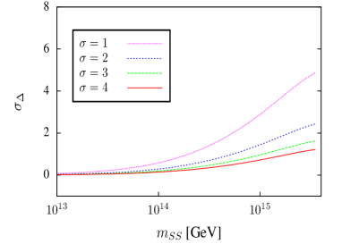
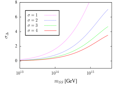
Figure 3: Calculated $\chi^{2}$ for the observable $\Delta(m_{\tilde{e}\tilde{\mu}})$ as function of $m_{SS}$ for different values of its error. To the left: $P_{1}$; to the right $P_{5}$.

Fig. (2) also demonstrates that $\Delta(m_{\tilde{e}\tilde{\mu}})$ at its nominal error gives a significant contribution to the total $\chi^{2}$. Thus, LHC measurements only might already give some hints for a type-I seesaw Abada:2010kj . However, with the rather large error bars of mass measurements at the LHC it will not be possible to fix the cMSSM parameters with sufficient accuracy to get a reliable error on the value of $m_{SS}$. Unfortunately, also the accuracy with which $\Delta(m_{\tilde{e}\tilde{\mu}})$ can be measured at the LHC is quite uncertain. According to Allanach:2008ib such a splitting could be found for values as low as (few) $10^{-4}$ or as large as (several) percent, depending on the kinematical configuration realized in nature. Moreover, our points $P_{1}$-$P_{5}$ have heavier spectra than the ones studied in Allanach:2008ib , so larger statistical errors are to be expected.

Fig. (3) shows the relative deviation of $\Delta(m_{\tilde{e}\tilde{\mu}})$ for $P_{1}$ (left) and $P_{5}$ (right) for different assumed values of the error in this observable, relative to cMSSM. Here, $\sigma=1,2,3,4$ means that we have multiplied the “error” quoted in Allanach:2008ib by factors $1,2,3,4$. The deviation drops below one sigma for any value of $m_{SS}$ shown for $P_{1}$ ($P_{5}$) when this error is larger than twice (six times) the nominal error. This implies that no hints for seesaw type-I can be found in LHC data if the error on $\Delta(m_{\tilde{e}\tilde{\mu}})$ is larger than 5 $\permil$ (1.6 %) in case of $P_{1}$ ($P_{5}$).

We should also mention that the actual value of $\Delta(m_{\tilde{e}\tilde{\mu}})$ is not only a function of $m_{SS}$ and the cMSSM parameters, but also depends on the type of fit used to explain neutrino data. We have used degenerate right-handed neutrinos and $m_{\nu_{1}}\equiv 0$ in the plots shown above. Much smaller splittings are found for (a) nearly-degenerate light neutrinos, i.e. $m_{\nu_{1}}\geq 0.05$ eV; or (b) very hierarchical right-handed neutrinos. We have checked by an explicit calculation that, for example, for $P_{5}$ and $m_{\nu_{1}}\equiv 0$, $\Delta\chi^{2}\geq 5.89$ for values of $m_{SS}$ larger than $m_{SS}\simeq 1.6\times 10^{14}$ GeV from $\Delta(m_{\tilde{e}\tilde{\mu}})$ alone, whereas the same $\Delta\chi^{2}$ is reached for $m_{\nu_{1}}=0.05$ eV only for $m_{SS}\raise 1.29167pt\hbox{$\;>$\kern-7.5pt\raise-4.73611pt\hbox{$\sim\;$}}7\times 10^{14}$ GeV. Consequently, even though one expects that a finite mass difference between left smuon and selectron is found in cMSSM type-I seesaw, this is by no means guaranteed.

Similar comments apply to the errors for the selectron and smuon mass at the ILC. For $P_{1}$ ($P_{5}$) the departure of the left selectron mass from the cMSSM expectations is smaller than 1 $\sigma$ even for $m_{SS}\sim 3\times 10^{15}$ if the error on this mass is larger than $1.5\permil$ ($1\%$). For the left smuon the corresponding numbers are for $P_{1}$ and $P_{5}$ approximately $1.5\%$ and $5\%$, respectively.

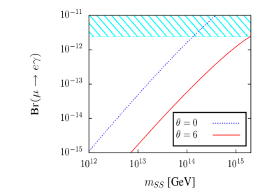
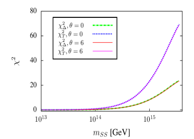
Figure 4: To the left Br($\mu\to e\gamma$) and to right calculated $\chi^{2}$ as function of $m_{SS}$ for two different values of the reactor angle $\theta_{R}$.

Naively one expects LFV violation to be large, whenever the neutrino Yukawa couplings are large, i.e. for large values of $m_{SS}$. That is, the regions testable by SUSY mass measurements could already be excluded by upper bounds on LFV, especially the recent upper bound on $\mu\to e\gamma$ by MEG arXiv:1107.5547 . That this conjecture is incorrect is demonstrated by the example shown in fig. (4). In this figure we show the calculated Br($\mu\to e\gamma$) to the left and the calculated $\chi^{2}$ (total and only $\Delta(m_{\tilde{e}\tilde{\mu}})$) to the right for $\delta=\pi$ and two different values of the reactor angle, $\theta_{13}$ for the point $P_{1}$. For $\theta_{13}=0$ all values of $m_{SS}$ above approximately $m_{SS}\sim 10^{14}$ GeV are excluded by the upper bound Br($\mu\to e\gamma$) $\leq 2.4\times 10^{-12}$ arXiv:1107.5547 . For $\theta_{13}=6^{\circ}$ nearly all values of $m_{SS}$ become allowed. At the same time, this “small” change in the Yukawas has practically no visible effect on the calculated $\chi^{2}$ from mass measurements as the plot on the right shows. This demonstrates that SUSY mass measurements and LFV probe different portions of seesaw type-I parameter space, contrary to what is sometimes claimed in the literature. That one can fit LFV and SUSY masses independently even for such a simple model as type-I seesaw is already obvious from eq. (13): Even after fixing all low energy neutrino observables we still have nine unknown parameters to choose from to fit any entry of the left slepton masses independently.

Fig. (4) also shows that non-zero values of $\theta_{13}$, as preferred by the most recent experimental data arXiv:1111.0183 ; DC2011 , should have very little effect on our parameter scans. In our numerical scans, discussed next, we therefore keep $\theta_{13}=0$ unless mentioned otherwise. We will, however, also briefly comment on changes of our results, when $\theta_{13}$ is allowed to float within its current error.

III.3 Numerical scans

For the determination of errors on the cMSSM parameters and $m_{SS}$ we have used two independent programmes, one based on MINUIT while the other uses a simple MonteCarlo procedure to scan over the free parameters. For a more detailed discussion see Hirsch:2011cw . Plots shown below are obtained by the MonteCarlo procedure, but we have checked that results from MINUIT and our simplistic approach described above give very similar estimates for the $\chi^{2}$, with MINUIT only slightly improving the quality of the fit. In this section we always use all observables in the fits and quote all errors at 1 $\sigma$ c.l., unless noted otherwise. Since our “fake” experimental data sets are perfect sets, the minimum of $\chi^{2}$ calculated equals zero and is thus not meaningful; only $\Delta\chi^{2}$ calculated with respect to the best fit points has any physical meaning in the plots shown below.

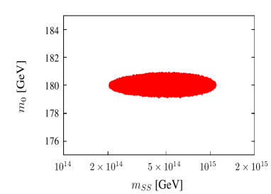
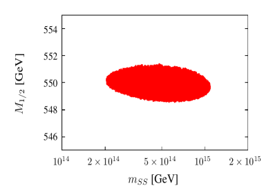
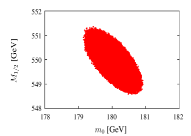
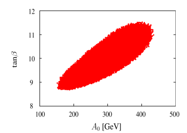
Figure 5: Calculated allowed parameter space for $m_{0}$, $M_{1/2}$, $\tan\beta$, $A_{0}$ and $m_{SS}$ for 7 free parameters, $P_{5}$ and $m_{SS}=5\times 10^{14}$ GeV. For discussion see text.

Fig. (5) shows the allowed parameter space obtained in a MonteCarlo run for $m_{0}$, $M_{1/2}$, $\tan\beta$, $A_{0}$ and $m_{SS}$ for 7 free parameters, $P_{5}$ and $m_{SS}=5\times 10^{14}$ GeV. Shown are the allowed ranges of $m_{0}$ and $M_{1/2}$ versus $m_{SS}$, as well as $m_{0}$ versus $M_{1/2}$ and $\tan\beta$ versus $A_{0}$. On top of the 4 cMSSM parameters and $m_{SS}$ in this calculation we allow the solar angle ($\theta_{12}$) and the atmospheric angle ($\theta_{23}$) to float freely within their allowed range. Errors on neutrino angles for this plot are taken from arXiv:1103.0734 . Plots for other points and/or different sets of free parameters look qualitatively very similar to the example shown in the figure. There is very little correlation among different parameters, contrary to the situation found in case of seesaw type-II and type-III Hirsch:2011cw . Especially no correlations between $m_{0}$, $M_{1/2}$ and $m_{SS}$ are found. However, there is some correlation between $\tan\beta$ and $A_{0}$, driven by the fact that $m_{h^{0}_{1}}$ alone can only fix a certain combination of these two parameters well. The correlation between $\tan\beta$ and $A_{0}$ is slightly stronger than in the cMSSM case, due to the contribution of $A_{0}$ in the running of slepton masses, see eq. (13).

For our assumed set of measurements, $m_{0}$ and $M_{1/2}$ are mainly determined by the highly accurate measurements of right slepton and gaugino masses of the ILC. $A_{0}$ and $\tan\beta$ are fixed by a combination of the lightest Higgs mass and the lighter stau mass. LHC measurements help to break degeneracies in parameter space, but are much less important. We stress that the highly accurate determination of cMSSM parameters shown in fig. (5) is a prerequisite for determining reliable errors on $m_{SS}$.

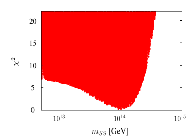
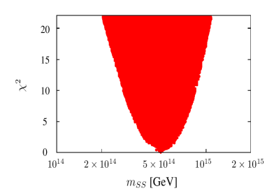
Figure 6: Calculated $\chi^{2}$ distribution versus $m_{SS}$ for 7 free parameters, $P_{5}$ and $m_{SS}=10^{14}$ GeV (to the left) and $m_{SS}=5\times 10^{14}$ GeV (to the right).

Fig. (6) shows calculated $\chi^{2}$ distributions versus $m_{SS}$ for the same 7 free parameters as in fig. (5), $P_{5}$ and $m_{SS}=10^{14}$ GeV (to the left) and $m_{SS}=5\times 10^{14}$ GeV (to the right). For the latter an upper (lower) limit of $m_{SS}\simeq 8\times 10^{14}$ GeV ($m_{SS}\simeq 3\times 10^{14}$ GeV) is found. For $m_{SS}=10^{14}$ GeV a clear upper limit is found, but for low values of $m_{SS}$ the $\chi^{2}$ distribution flattens out at $\Delta\chi^{2}\sim 6.5$. This different behaviour can be understood with the help of the results of the previous subsection, see fig. (2). For $m_{SS}=5\times 10^{14}$ GeV, there exists a notable difference in some observables with respect to the cMSSM expectation, especially left smuon and selectron mass can no longer be adequately fitted by varying $m_{0}$ and $M_{1/2}$ alone, without destroying the agreement with “data” for right sleptons and gauginos. Therefore both, a lower and an upper limit on $m_{SS}$ exist for this point. The situation is different for $m_{SS}=10^{14}$ GeV, for which the spectrum is much closer to cMSSM expectations. Larger values of $m_{SS}$ are excluded, since they would require larger Yukawas, i.e. larger deviation from cMSSM than observed. Smaller values of $m_{SS}$, on the other hand, have ever smaller values of $Y^{\nu}$, i.e. come closer and closer to cMSSM expectations. For an input value of $m_{SS}$ just below $m_{SS}=10^{14}$ GeV there is then no longer any lower limit on $m_{SS}$, i.e. the data becomes perfectly consistent with a pure cMSSM calculation. In this case one can only “exclude” a certain range of the seesaw, say values of $m_{SS}$ above a few $10^{14}$ GeV.

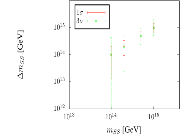
Figure 7: Calculated allowed range of $m_{SS}$ versus $m_{SS}$ for 5 (left) and 7 (right) free parameters and $P_{5}$. The two different error bars correspond to 1 and 3 $\sigma$ c.l.

One standard deviation is, of course, too little to claim an observation. We therefore show in fig. (7) $\Delta(m_{SS})$ versus $m_{SS}$ for 5 (left) and 7 (right) free parameters and $P_{5}$ at 1 and 3 $\sigma$ c.l. At $m_{SS}=10^{14}$ formally a 1 sigma “evidence” could be reached, but at 3 $\sigma$ c.l. the spectrum is perfectly consistent with a pure cMSSM. For larger values of $m_{SS}$, however, several standard deviations can be reached. For the two largest values of $m_{SS}$ calculated in this figure, a 5 $\sigma$ “discovery” is possible.

Fig. (7) shows $\Delta(m_{SS})$ for 5 and 7 free parameters. We have repeated this exercise for different sets of free parameters and $m_{SS}=5\times 10^{14}$. Here, 5 free parameters correspond to the 4 cMSSM parameters plus $m_{SS}$, 7 free parameters are the original 5 plus $\theta_{12}$ and $\theta_{23}$. We have also tried other combinations such as 6 parameters: original 5 plus $\theta_{R}$ and 8 parameters, where we let all 3 neutrino angles float freely. Sets with larger numbers of free parameters are no longer sufficiently sampled in our MonteCarlo runs, so we do not give numbers for these, although in principle the calculation could allow also to let the neutrinos mass squared differences to float freely. Error bars are slightly larger for larger number of free parameters, as expected. However, since there is little or no correlation among the parameters, the differences are so small as to be completely irrelevant.

IV Summary and discussion

We have discussed the prospects for finding indirect hints for type-I seesaw in SUSY mass measurements. Since type-I seesaw adds only singlets to the SM particle content, only very few observables are affected and all changes in masses are small, even in the most favourable circumstances. Per-mille level accuracies will be needed, i.e. measurements at an ILC, before any quantitative attempt searching for type-I seesaw can hope for success, even assuming admittedly simplistic cMSSM boundary condtions.

Our calculation confirms quantitatively that slepton mass measurements can contain information about the type-I seesaw. Right sleptons are expected to be degenerate, while the left smuon and selectron show a potentially measurable splitting between their masses. If such a situation is indeed found, an estimate of $m_{SS}$ might be derivable from ILC SUSY mass measurements.

Above we have commented only on experimental errors. However, given the per-mille requirements on accuracy, stressed several times, also theoretical errors in the calculation of SUSY spectra are important. Various potential sources of errors come to mind. First of all, a 1-loop calculation of SUSY masses is almost certainly not accurate enough for our purposes. We have tried to estimate the importance of higher loop orders, varying the renormalization scale in the numerical calculation. Changes of smuon and selectron mass found are of the order of the ILC error or even larger, depending on SUSY point and variation of scale. For the mass of the lightest Higgs boson it has been shown that even different calculations at 2-loop still disagree at a level of few GeV hep-ph/0406166 . Second, our calculation assumes a perfect knowledge of the GUT scale. Changes in the GUT scale do lead to sizeable changes in the calculated spectra for the same cMSSM parameters, which can be easily of the order of the required precision of the calculation and larger. In this sense, $\Delta(m_{\tilde{e}\tilde{\mu}})$ is an especially nice observable, since here the GUT scale uncertainty nearly cancels out in the calculation. In summary, if ILC accuracies on SUSY masses can indeed be reached experimentally, progress on the theoretical side will become necessary too.

In our calculations, we have considered only SUSY masses. We have not taken into account data from lepton flavour violation, mainly because currently only upper limits are available. If in the future finite values for $\l_{i}\to\l_{j}+\gamma$ become available, it would be very interesting to see, how much could be learned about the type-I seesaw parameters in a combined fit. Including LFV one could maybe also allow for non-degenerate right-handed neutrinos in the fits.

And, finally, despite all the limitations of our study, we find it very encouraging that hints for type-I seesaw might be found in SUSY mass measurements at all. We stress again, that LFV and SUSY mass measurements test different portions of seesaw parameter space. For a more complete “reconstruction” of seesaw parameters, than what we have attempted here, both kinds of measurements would be needed.

References

- (1) P. Minkowski, Phys. Lett. B 67 (1977) 421.
- (2) T. Yanagida, in KEK lectures, ed. O. Sawada and A. Sugamoto, KEK, 1979; M Gell-Mann, P Ramond, R. Slansky, in Supergravity, ed. P. van Niewenhuizen and D. Freedman (North Holland, 1979);
- (3) R.N. Mohapatra and G. Senjanovic, Phys. Rev. Lett. 44 912 (1980).
- (4) J. Schechter and J. W. F. Valle, Phys. Rev. D 22, 2227 (1980).
- (5) T. P. Cheng and L. F. Li, Phys. Rev. D 22, 2860 (1980).
- (6) Y. Fukuda et al. [Super-Kamiokande Collaboration], Phys. Rev. Lett. 81, 1562 (1998)
- (7) SNO, Q. R. Ahmad et al., Phys. Rev. Lett. 89, 011301 (2002), [nucl-ex/0204008].
- (8) KamLAND, K. Eguchi et al., Phys. Rev. Lett. 90, 021802 (2003), [hep-ex/0212021].
- (9) S. Abe et al. [KamLAND Collaboration], Phys. Rev. Lett. 100, 221803 (2008) [arXiv:0801.4589 [hep-ex]].
- (10) For a recent review on the status of neutrino oscillation data, see: T. Schwetz, M. A. Tortola and J. W. F. Valle, New J. Phys. 10, 113011 (2008) [arXiv:0808.2016 [hep-ph]]. Version 3 on the arXive is updated with data until Feb 2010
- (11) K. Nakamura et al. [Particle Data Group], J. Phys. G 37 (2010) 075021.
- (12) R. N. Mohapatra and J. W. F. Valle, Phys. Rev. D34, 1642 (1986).
- (13) E. Akhmedov, M. Lindner, E. Schnapka and J. W. F. Valle, Phys. Rev. D53, 2752 (1996), [hep-ph/9509255]; Phys. Lett. B368, 270 (1996), [hep-ph/9507275].
- (14) F. Borzumati and A. Masiero, Phys. Rev. Lett. 57, 961 (1986).
- (15) J. Hisano, T. Moroi, K. Tobe, M. Yamaguchi and T. Yanagida, Phys. Lett. B 357, 579 (1995) [arXiv:hep-ph/9501407].
- (16) J. Hisano, T. Moroi, K. Tobe and M. Yamaguchi, Phys. Rev. D 53, 2442 (1996) [arXiv:hep-ph/9510309].
- (17) J. R. Ellis, J. Hisano, M. Raidal and Y. Shimizu, Phys. Rev. D 66, 115013 (2002) [arXiv:hep-ph/0206110].
- (18) F. Deppisch, H. Pas, A. Redelbach, R. Ruckl and Y. Shimizu, Eur. Phys. J. C 28, 365 (2003) [arXiv:hep-ph/0206122].
- (19) E. Arganda and M. J. Herrero, Phys. Rev. D 73, 055003 (2006) [arXiv:hep-ph/0510405].
- (20) S. Antusch, E. Arganda, M. J. Herrero and A. M. Teixeira, JHEP 0611, 090 (2006) [arXiv:hep-ph/0607263].
- (21) E. Arganda, M. J. Herrero and A. M. Teixeira, JHEP 0710, 104 (2007) [arXiv:0707.2955 [hep-ph]].
- (22) J. Hisano, M. M. Nojiri, Y. Shimizu and M. Tanaka, Phys. Rev. D 60, 055008 (1999) [arXiv:hep-ph/9808410].
- (23) G. A. Blair, W. Porod and P. M. Zerwas, Eur. Phys. J. C27, 263 (2003), [hep-ph/0210058].
- (24) A. Freitas, W. Porod and P. M. Zerwas, Phys. Rev. D72, 115002 (2005), [hep-ph/0509056].
- (25) S. T. Petcov, S. Profumo, Y. Takanishi and C. E. Yaguna, Nucl. Phys. B 676 (2004) 453 [arXiv:hep-ph/0306195]; S. Pascoli, S. T. Petcov and C. E. Yaguna, Phys. Lett. B 564 (2003) 241 [arXiv:hep-ph/0301095]; S. T. Petcov, T. Shindou and Y. Takanishi, Nucl. Phys. B 738 (2006) 219 [arXiv:hep-ph/0508243]; S. T. Petcov and T. Shindou, Phys. Rev. D 74 (2006) 073006 [arXiv:hep-ph/0605151].
- (26) M. Hirsch, J. W. F. Valle, W. Porod, J. C. Romao and A. Villanova del Moral, Phys. Rev. D 78, 013006 (2008) [arXiv:0804.4072 [hep-ph]].
- (27) M. Hirsch, Nucl. Phys. Proc. Suppl. 217, 318 (2011).
- (28) R. Foot, H. Lew, X. G. He and G. C. Joshi, Z. Phys. C 44, 441 (1989).
- (29) E. Ma, Phys. Rev. Lett. 81, 1171 (1998) [arXiv:hep-ph/9805219].
- (30) A. Rossi, Phys. Rev. D 66, 075003 (2002) [arXiv:hep-ph/0207006].
- (31) M. Hirsch, S. Kaneko and W. Porod, Phys. Rev. D 78, 093004 (2008) [arXiv:0806.3361 [hep-ph]].
- (32) J. N. Esteves, J. C. Romao, M. Hirsch, F. Staub and W. Porod, Phys. Rev. D 83, 013003 (2011) [arXiv:1010.6000 [hep-ph]].
- (33) C. Biggio and L. Calibbi, arXiv:1007.3750 [hep-ph].
- (34) M. R. Buckley and H. Murayama, Phys. Rev. Lett. 97, 231801 (2006) [arXiv:hep-ph/0606088].
- (35) V. De Romeri, M. Hirsch and M. Malinsky, Phys. Rev. D 84, 053012 (2011) [arXiv:1107.3412 [hep-ph]].
- (36) G. Weiglein et al. [LHC/LC Study Group], Phys. Rept. 426 (2006) 47 [arXiv:hep-ph/0410364].
- (37) J. A. Aguilar-Saavedra et al., Eur. Phys. J. C 46, 43 (2006) [arXiv:hep-ph/0511344].
- (38) M. Hirsch, L. Reichert, W. Porod, JHEP 1105, 086 (2011). [arXiv:1101.2140 [hep-ph]].
- (39) J. A. Aguilar-Saavedra et al. [ECFA/DESY LC Physics Working Group], arXiv:hep-ph/0106315.
- (40) F. Deppisch, A. Freitas, W. Porod and P. M. Zerwas, Phys. Rev. D 77 (2008) 075009 [arXiv:0712.0361 [hep-ph]].
- (41) K. Kadota and J. Shao, Phys. Rev. D 80 (2009) 115004 [arXiv:0910.5517 [hep-ph]].
- (42) A. Abada, A. J. R. Figueiredo, J. C. Romao and A. M. Teixeira, JHEP 1010, 104 (2010) [arXiv:1007.4833 [hep-ph]].
- (43) B. C. Allanach, J. P. Conlon and C. G. Lester, Phys. Rev. D 77, 076006 (2008) [arXiv:0801.3666 [hep-ph]].
- (44) J. A. Casas and A. Ibarra, Nucl. Phys. B 618, 171 (2001) [arXiv:hep-ph/0103065].
- (45) S. P. Martin and M. T. Vaughn, Phys. Rev. D 50, 2282 (1994) [Erratum-ibid. D 78, 039903 (2008)] [arXiv:hep-ph/9311340].
- (46) R. Fonseca, M. Malinsky, W. Porod and F. Staub, arXiv:1107.2670 [hep-ph].
- (47) W. Porod, Comput. Phys. Commun. 153 (2003) 275 [arXiv:hep-ph/0301101].
- (48) W. Porod and F. Staub, arXiv:1104.1573 [hep-ph].
- (49) P. F. Harrison, D. H. Perkins and W. G. Scott, Phys. Lett. B 530, 167 (2002) [hep-ph/0202074].
- (50) M. Khabibullin and f. t. T. Collaboration, arXiv:1111.0183 [hep-ex].
- (51) Double CHOOZ experiment, talk by H.De. Kerrect at LowNu2011, http://workshop.kias.re.kr/lownu11/
- (52) H. Bachacou, I. Hinchliffe and F. E. Paige, Phys. Rev. D 62 (2000) 015009 [arXiv:hep-ph/9907518].
- (53) B. C. Allanach, C. G. Lester, M. A. Parker and B. R. Webber, JHEP 0009 (2000) 004 [arXiv:hep-ph/0007009].
- (54) C. G. Lester, “Model independent sparticle mass measurements at ATLAS”; CERN-THESIS-2004-003
- (55) S. Chatrchyan et al. [CMS Collaboration], Phys. Rev. Lett. 107 (2011) 221804; arXiv:1109.2352 [hep-ex].
- (56) G. Aad et al. [ATLAS Collaboration], arXiv:1109.6572 [hep-ex].
- (57) B. C. Allanach et al., in Proc. of the APS/DPF/DPB Summer Study on the Future of Particle Physics (Snowmass 2001) ed. N. Graf, Eur. Phys. J. C 25, 113 (2002) [arXiv:hep-ph/0202233].
- (58) G. Belanger, F. Boudjema, P. Brun, A. Pukhov, S. Rosier-Lees, P. Salati and A. Semenov, Comput. Phys. Commun. 182, 842 (2011) [arXiv:1004.1092 [hep-ph]].
- (59) G. Belanger, F. Boudjema, A. Pukhov and A. Semenov, Comput. Phys. Commun. 180, 747 (2009) [arXiv:0803.2360 [hep-ph]].
- (60) G. Belanger, F. Boudjema, A. Pukhov and A. Semenov, Comput. Phys. Commun. 176, 367 (2007) [hep-ph/0607059].
- (61) G. Belanger, F. Boudjema, A. Pukhov and A. Semenov, Comput. Phys. Commun. 174, 577 (2006) [hep-ph/0405253].
- (62) J. Adam et al. [MEG Collaboration], Phys. Rev. Lett. 107, 171801 (2011) [arXiv:1107.5547 [hep-ex]].
- (63) T. Schwetz, M. Tortola and J. W. F. Valle, New J. Phys. 13, 063004 (2011) [arXiv:1103.0734 [hep-ph]].
- (64) B. C. Allanach, A. Djouadi, J. L. Kneur, W. Porod and P. Slavich, JHEP 0409, 044 (2004) [hep-ph/0406166].