Asymptotic scattering and duality in the one-dimensional three-state quantum Potts model on a lattice

Abstract

We determine numerically the single-particle and the two-particle spectrum of the three-state quantum Potts model on a lattice by using the density matrix renormalization group method, and extract information on the asymptotic (small momentum) S-matrix of the quasiparticles. The low energy part of the finite size spectrum can be understood in terms of a simple effective model introduced in a previous work, and is consistent with an asymptotic S-matrix of an exchange form below a momentum scale $p^{*}$. This scale appears to vanish faster than the Compton scale, $mc$, as one approaches the critical point, suggesting that a dangerously irrelevant operator may be responsible for the behavior observed on the lattice.

1 Introduction

Being the simplest generalization of the transverse field Ising model, the $q$ state quantum Potts model is one of the most paradigmatic models in statistical physics and quantum field theory. The case of $q=3$ is somewhat peculiar and is also of particular interest. On a regular one dimensional lattice, the $q=3$ state quantum Potts model displays a second order quantum phase transition between a ferromagnetic state and a paramagnetic state, just as the transverse field Ising model [1, 2, 3]. The properties of the critical state itself are very well characterized: at the critical point, an exact solution is available [4], and the scaling limit is known to be described in conformal field theory (CFT) by the minimal model of central charge $C=4/5$ [5, 6, 7, 8], with the so-called $D_{4}$ partition function [9]. The ordered and disordered phases of the quantum Potts model are, on the other hand, much richer than those of the transverse field Ising model: Similar to e.g. antiferromagnetic chains of integer spins [10, 11, 12], the gapped phases (i.e., the ferromagnetic as well as the paramagnetic phase) possess excitations with internal quantum numbers; as a consequence, the dynamics of these quasiparticles are much richer than those of the transverse field Ising model and, in contrast to the critical behavior, the quasiparticle properties of the gapped phases of the quantum Potts chain are not entirely understood.

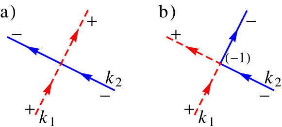
Figure 1: (Color online) Structures of the asymptotic S-matrices. a) Diagonal S-matrix. b) Exchange S-matrix.

In the continuum limit, the properties of the Potts model are usually described by the so-called scaling Potts field theory, which is a perturbation of the fixed point conformal field theory, uniquely determined by the symmetries. In this approach, the cut-off (lattice spacing) is removed, and only the leading relevant operator is kept. The application of the machinery known as the S-matrix bootstrap [13] yields a diagonal quasiparticle S-matrix for low energy particles [14, 15, 16, 17, 18, 19] and implies that the internal quantum numbers of two colliding particles are conserved during a scattering process (see fig. 1.a). The bootstrap S-matrix and the perturbed conformal field theory yield a fully consistent picture [20].

Recent perturbative calculations as well as renormalization group arguments showed [3], on the other hand, that rather than being diagonal, the asymptotic S-matrix of the lattice Potts model assumes the ”universal” form, also emerging in various spin models [11], as well as in the sine-Gordon model [13]: $\hat{S}\to-\hat{X}$, with $\hat{X}$ the exchange operator (see fig. 1.b). Although the arguments of Ref. [3] are very robust, the results of Ref. [3] were met by some skepticism. On the one hand, the lattice results seemed to conflict with results obtained within the scaling Potts theory [13, 15, 16, 17, 18, 19]. On the other hand, various thermodynamical properties of the two dimensional classical Potts model (on a lattice) such as critical exponents [7] or universal amplitude ratios [38, 39] also seem to agree with the predictions of the scaling Potts model (perturbed $C=4/5$ minimal model). We must emphasize that the structure of the asymptotic S-matrix has important physical consequences: an S-matrix of the exchange form yields diffusive finite temperature spin-spin correlation functions at intermediate times [3, 21, 22], while a diagonal S-matrix would result in exponentially damped correlations [12, 23, 24].

The purpose of the present paper is to investigate and possibly resolve this apparent controversy. We study in detail the two-particle spectrum of the $q=3$ state quantum Potts chain using the powerful numerical method of density matrix renormalization group (DMRG). We find that the finite size spectra are indeed in complete agreement with the theory of Ref. [3] and an asymptotic (i.e., $k\to 0$ momentum) S-matrix of the exchange form. However, our analysis also reveals the emergence of a new momentum scale, $p^{*}$, below which this exchange S-matrix dominates. By approaching the critical point, this scale vanishes faster than the Compton momentum, $mc$, suggesting that the new scale and the corresponding exchange scattering is generated by some dangerously irrelevant operator, usually neglected in the scaling Potts model. Although our numerics are not accurate enough for large momenta, they are not inconsistent with a diagonal S-matrix as expected within the irrelevant-operator scenario for $|k|\gg p^{*}$.

2 The Potts model and its quasiparticles

In its lattice version, the Potts model consists of a chain of generalized spins having internal quantum states $|\mu\rangle_{i}$, with $i$ labeling the lattice sites and $\mu=1,\dots,q$ the possible internal states of the spins. The Hamiltonian of the $q$-state quantum Potts chain is then defined as

$$H=-J\sum_{i}\sum_{\mu=1}^{q}P^{\mu}_{i}P^{\mu}_{i+1}-Jg\sum_{i}P_{i}\;.$$ (1)

Here the traceless operators $P_{i}^{\mu}=|\mu\rangle_{i\,i}\langle\mu|-1/q$ tend to project the spin at site $i$ along the ”direction” $\mu$, and thus the first term of eq. (1) promotes a ferromagnetic ground state, with all spins spontaneously polarized in one of the directions, $|\mu\rangle$. In contrast, the second term in eq. (1) represents a ”transverse field”, with the traceless operator $P_{i}=|\lambda_{0}\rangle_{i\,i}\langle\lambda_{0}|-1/q$ trying to align the spins along the direction $|\lambda_{0}\rangle\equiv\sum_{\mu}|\mu\rangle/\sqrt{q}$. The relative strength of these two terms is regulated by the dimensionless coupling, $g$. These terms obviously compete with each other, and their competition leads to a phase transition: for large values of $g$ one finds a paramagnetic phase with a unique ground state, while for small $g$ a ferromagnetic phase appears with $q$ degenerate ground states, spontaneously breaking the global ${\mathbb{S}}_{q}$ symmetry. In the $q=3$ case,— on which we focus here,— the transition occurs at a coupling $g=g_{c}=1$, and it is of second order: quasiparticles are gapped on both sides of the transition, but the quasiparticle gap $\Delta$ vanishes continuously at the transition as $\Delta\sim J\;|g-1|^{5/6}$ [3].

The $q$ state Potts model obviously possesses a global ${\mathbb{S}}_{q}$ permutation symmetry. As a consequence, the global cyclic permutation $\mathcal{Z}|\mu\rangle_{i}=|\mu+1\;{\rm mod}\;q\rangle_{i}$ leaves the Hamiltonian also invariant, and can be used to classify its eigenstates as

$$\mathcal{Z}|Q\rangle=e^{i\Omega Q}|Q\rangle,$$ (2)

with $Q$ an integer and the angle $\Omega$ defined as $\Omega=2\pi/q$. We note that this holds even in the ferromagnetic phase, but there states with spontaneously broken symmetries must be mixed. In the particular case of $q=3$, considered here, $Q$ can take values of $Q=0$ and $Q=\pm$. In this case, pairwise spin exchanges (e.g., $\mu=1\leftrightarrow 2$) also imply that states with quantum numbers $Q=\pm$ come in degenerate pairs.

The structure of quasiparticles in the ferromagnetic ($g<1$) and in the paramagnetic ($g>1$) phases can be easily understood in the perturbative limits, $g\ll 1$ and $g\gg 1$. For $g>1$ the ground state $|0)$ is unique, and quasiparticles consist of local spin flips of ${\mathbb{S}}_{3}$ charges $Q=\pm$. For $g<1$, on the other hand, the ground state is 3-fold degenerate, $|0)\to|0)_{\mu}$, and quasiparticles correspond to domain walls between these ground states, $\mu\to\mu^{\prime}=\mu+\theta\;{\rm mod}\;3$, with $\theta=\pm$ the quantum number of the domain wall.

Similar to the Ising model, the Potts model is known to be self-dual. High-temperature – low-temperature duality [25] in the $d=2$ classical Potts model implies a duality $g\leftrightarrow 1/g$ for the quantum Potts chain [26]. In the Appendix we show that duality holds even on the level of the matrix elements of the Hamiltonian, and therefore one can map the spectra in the $Q=0$ sectors for $g$ and $1/g$ by simply rescaling the energies with appropriate factors. We thus have

$$E_{n}^{Q=0}(g)=g\;E_{n}^{Q=0}(1/g)$$ (3)

for all eigenstates $n$ with periodic boundary conditions (PBC), as also verified later numerically. This duality relation has important consequences, and shall allow us to relate various energy- and length scales on the two sides of the transition.

3 Effective theory and two-particle S-matrix

In an infinite system, the elementary excitations of the gapped phases can be classified by their momentum, $k$, and for small momenta their energy can be approximated as

$$\epsilon(k)=\Delta+\frac{k^{2}}{2m}+\dots\;$$ (4)

independently of their internal quantum number. Here $m=m(g)$ is the quasiparticle mass, and $\Delta=\Delta(g)$ denotes the quasiparticle gap.

In the very dilute limit, interactions between quasiparticles can be described in terms of just two-body collisions, and correspondingly, by just two-body scattering matrices and interactions. Assuming pairwise and short ranged interactions between the quasiparticles, one thus arrives at the following effective Hamiltonian (in first quantized form) [3, 12],

$${\cal H}=\sum_{i=1}^{N_{qp}}(\Delta-\frac{1}{2m}\frac{\partial^{2}}{\partial x_{i}^{2}})+\sum_{i<j}{u}^{\sigma_{i}^{\prime},\sigma_{j}^{\prime}}_{\sigma_{i},\sigma_{j}}(x_{i}-x_{j})+\dots\;,$$ (5)

with $x_{i}$ and $\sigma_{i}$ denoting the coordinates and internal quantum numbers of the quasiparticles, and $N_{qp}$ their number. The above Hamiltonian acts on many-particle wave functions $\psi_{\{\sigma_{i}\}}(\{x_{i}\})$, which are bosonic (invariant under exchanges $(x_{i},\sigma_{i})\leftrightarrow(x_{j},\sigma_{j})$), and correspond to states of the form $|\psi)=\sum_{\{x_{i}\}}\sum_{\{\sigma_{i}\}}\psi_{\{\sigma_{i}\}}(\{x_{i}\})|\{x_{i}\},\{\sigma_{i}\})$. The dots in eq. (5) denote higher order terms, which are irrelevant in the renormalization group sense, and do not influence the asymptotic low-energy properties of the theory.

The scattering of two quasiparticles on each other can be characterized by the two-particle S-matrix, which, in view of the energy and momentum conservation, has a simple structure. The two-particle S-matrix, in particular, relates the amplitude of an incoming asymptotic wave function $\psi_{k_{1}\sigma_{1},k_{2}\sigma_{2}}(x_{1}\ll x_{2})\approx A_{\sigma_{1},\sigma_{2}}^{\rm in}(k_{1},k_{2})e^{i(k_{1}x_{1}+k_{2}x_{2})}$ with quasiparticle momenta $k_{1}>k_{2}$ to that of the outgoing wave function, $\psi_{k_{1}\sigma_{1},k_{2}\sigma_{2}}(x_{1}\gg x_{2})\approx B_{\sigma_{1},\sigma_{2}}^{\rm out}(k_{1},k_{2})e^{i(k_{1}x_{1}+k_{2}x_{2})}$ as

$${\bf B}^{\rm out}={\hat{S}}(k_{1}-k_{2})\;{\bf A}^{\rm in}\;.$$ (6)

The structure of the two-body S-matrix is further restricted by ${\mathbb{S}}_{3}$ symmetry:

$${\hat{S}}(k)=\left(\begin{array}[]{cccc}s_{3}(k)&0&0&0\\ 0&s_{1}(k)&s_{2}(k)&0\\ 0&s_{2}(k)&s_{1}(k)&0\\ 0&0&0&s_{3}(k)\end{array}\right).$$ (7)

In the following, we shall only investigate the scattering of quasiparticles in the channels $\{+-\}$ and $\{-+\}$. In these channels, the eigenvalues of the S-matrix read

$$s_{t}(k) \equiv e^{2i\delta_{t}(k)}=s_{1}(k)+s_{2}(k)\;,$$ (8)

$$s_{s}(k) \equiv e^{2i\delta_{s}(k)}=s_{1}(k)-s_{2}(k)\;,$$ (9)

where we introduced the ”triplet” and ”singlet” eigenvalues, $s_{t}(k)$ and $s_{s}(k)$, and the corresponding phase shifts, $\delta_{t}(k)$ and $\delta_{s}(k)$. As shown in Ref. [3], interactions in the singlet channel are irrelevant for $k\to 0$ (the wave function has a node at $x_{1}=x_{2}$), while they are relevant in the triplet channel, unless some very special conditions are met by the effective interactions [3]. As a result, generically one finds $s_{t}(k\to 0)=-1$ while $s_{s}(k\to 0)=1$, as also confirmed by direct calculations in the $g\to\infty$ and $g\to 0$ limits [3]. As a consequence, by analyticity, the phase shifts must have the following small momentum expansion:

$$\delta_{t}(k)=-\frac{\pi}{2}\;{\rm sgn}(k)+a_{t}k+\dots\;,\phantom{nnn}\delta_{s}(k)=-a_{s}k+\dots\;.$$ (10)

Notice that these expressions (together with $s_{3}(k\to 0)=-1$) give rise to a low-momentum scattering matrix of the form, $\hat{S}\approx-\hat{X}$. In contrast, perturbed conformal field theory yields a diagonal low-momentum S-matrix with $s_{t}(k\to 0)=1$, corresponding to irrelevant interactions even in the triplet channel. However, this would require very special interactions, and is not guaranteed by ${\mathbb{S}}_{3}$ symmetry.

3.1 Two-particle spectra: paramagnetic phase

The two-particle spectrum of a finite system of size $L\gg a\equiv 1$ follows from the asymptotic form of the S-matrix. In the following, we shall focus exclusively on the simplest case of periodic boundary conditions (PBC).

In the paramagnetic phase, quasiparticles carry a “chirality” label, $\sigma=Q=\pm$. Therefore, the $Q=+$ sector of the spectrum contains single quasiparticle excitations of chirality $\sigma=+$ [described by eq. (4)] as well as, e.g., two-particle excitations with charges $\sigma_{1}=\sigma_{2}=-$. As a consequence, in the $Q=\pm$ sectors it is numerically hard to separate two-particle states from the single-particle states. We therefore focus on the sector $Q=0$, where single quasiparticle states are absent, and, above the ground state, the spectrum starts directly with two-particle eigenstates of quasiparticles with charges $\sigma_{1}=\pm$ and $\sigma_{2}=\mp$.

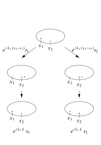
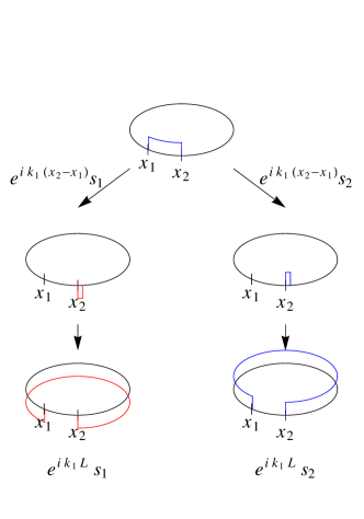
Figure 2: (Color online) Translating one of the quasiparticles around by system size $L$ in the paramagnetic (left figure) and ferromagnetic (right figure) phases.

For large system sizes, the quantization of the momenta $k_{1}$ and $k_{2}$ of the quasiparticles is determined by the periodicity condition on the wave function, $\Psi(x_{1},x_{2})\equiv\Psi(x_{1}+L,x_{2})\equiv\Psi(x_{1},x_{2}+L)$, and, just as in Bethe Ansatz, the energy is the sum of the two quasiparticle energies, $E=\epsilon(k_{1})+\epsilon(k_{2})$. Taking particle $i=1$ around the system (see fig. 2) then yields the following condition,

$$\left(\begin{array}[]{c}C_{1}\\ C_{2}\end{array}\right)=e^{ik_{1}L}\left(\begin{array}[]{cc}s_{1}(k_{1}-k_{2})&s_{2}(k_{1}-k_{2})\\ s_{2}(k_{1}-k_{2})&s_{1}(k_{1}-k_{2})\end{array}\right)\left(\begin{array}[]{c}C_{1}\\ C_{2}\end{array}\right)\;,$$ (11)

with $C_{1}=A_{+-}^{\rm in}(k_{1}\geq k_{2})$ and $C_{2}=A_{-+}^{\rm in}(k_{1}\geq k_{2})$ the wave function amplitudes for $0<x_{1}<x_{2}<L$, defined earlier. Taking particle $i=2$ around, $x_{2}\to x_{2}+L$, yields a similar equation. In the triplet channel, $C_{1}=C_{2}$, we thus obtain

$$s_{t}(k_{1}-k_{2})=e^{-ik_{1}L}\;,\phantom{nnn}s_{t}(k_{2}-k_{1})=e^{-ik_{2}L}\;.$$ (12)

Using the asymptotic expansions of the phase shifts, eq. (10), and solving eq. (12) to leading order in $1/L$ then gives

$$E_{n_{1},n_{2}}^{t}-2\,\Delta={{\cal E}_{0}}\;\left[\frac{1}{4}(n_{1}+n_{2})^{2}+\frac{1}{4}\frac{(n_{1}-n_{2}+1)^{2}}{(1+\frac{4a_{t}}{L})^{2}}+{\cal O}(1/L^{2})\right]\;,$$ (13)

where $n_{1}$ and $n_{2}$ denote integers, and we introduced the energy unit,

$${{\cal E}_{0}}\equiv\frac{1}{m}\left(\frac{2\pi}{L}\right)^{2}\;.$$ (14)

In eq. (13), to comply with the bosonic nature of the excitations, the quantum numbers $n_{1}$ and $n_{2}$ must satisfy $n_{1}\geq n_{2}$.

The previous analysis can be carried over to the singlet sector, $C_{1}=-C_{2}$, with little modification, and there it yields the following finite size spectrum:

$$E_{n_{1},n_{2}}^{s}-2\,\Delta={{\cal E}_{0}}\;\left[\frac{1}{4}(n_{1}+n_{2})^{2}+\frac{1}{4}\frac{(n_{1}-n_{2})^{2}}{(1-\frac{4a_{s}}{L})^{2}}+{\cal O}(1/L^{2})\right].$$ (15)

However, now $n_{1}$ and $n_{2}$ must satisfy $n_{1}>n_{2}$ since for $n_{1}=n_{2}$ the wave function vanishes trivially.

3.2 Two-particle spectra: ferromagnetic phase

As discussed earlier, the ground state of the infinite system in the ferromagnetic phase has broken ${\mathbb{S}}_{3}$ symmetry, and correspondingly, it is 3-fold degenerate, $|0)_{\mu}$. Here we use brackets rather than angular brackets, to explicitly emphasize that the states $|0)_{\mu}$ are interacting many-body eigenstates of the Hamiltonian. Excitations are kinks (domain walls), and the corresponding two-particle states read

$$|x_{1}\,\theta_{1},x_{2}\,\theta_{2})_{\mu}\;,$$ (16)

with $\mu$ the vacuum polarization at $x\to-\infty$, $x_{i}$ the positions of the domain steps, and $\theta_{i}=\pm$ the step sizes. As we shall also demonstrate later through our finite size spectrum analysis, by duality, the S-matrix of these kinks is identical to that of the local spin flip excitations on the paramagnetic side at a corresponding coupling, $g\to 1/g>1$.

On a ring, PBC implies that $\theta_{1}+\theta_{2}=0$. Furthermore, in contrast to the paramagnetic phase, in the ferromagnetic phase one must take into account the presence of the three possible vacuum states when constructing periodic solutions. A way to do that is by keeping track of the vacuum polarization at position $x=0$, e.g. As a consequence, wave function amplitudes must also have a vacuum label on the ring, $A_{\theta_{1}\theta_{2}}\to A_{\theta_{1}\theta_{2}}^{(\mu)}$. However, there is a subtle difference between scattering in an infinite system and scattering on the ring. As illustrated in fig. 2, moving one of the kinks around results not only in a phase change and a collision of the elementary excitations, but the domain orientations also change in a peculiar manner: the configuration essentially turns “inside out”. Correspondingly, the amplitudes of the wave functions change as

$$A_{+-}^{(\mu)}\to e^{ik_{1}L}\,s_{1}(k_{1}-k_{2})\;A_{+-}^{(\mu-1)}+e^{ik_{1}L}\,s_{2}(k_{1}-k_{2})\;A_{-+}^{(\mu+1)}\;.$$ (17)

The states discussed so far are not eigenstates of the cyclic operator, $\mathcal{Z}$ (cf. eq. (2)). However, we can define eigenstates of $\mathcal{Z}$ by taking linear combinations of them. Combining e.g. the three ferromagnetic ground states we find

$$|Q)=\frac{1}{\sqrt{3}}\sum_{\mu}e^{-i\Omega Q\mu}|0)_{\mu}\;.$$ (18)

Similarly, we can define the two-particle states, $|x_{1}\,\theta_{1},x_{2}\,\theta_{2};Q)$, and the corresponding scattering states and wave function amplitudes, $A^{Q}_{\theta_{1}\theta_{2}}$, by simply mixing the states and the wave function amplitudes as in eq. (18). Since the quantum number $Q$ is conserved, the periodicity condition of two-particle states simplifies in this basis. Taking the kink $i=1$ around the ring, the relation in eq. (17) implies the following equation for the amplitudes $C_{1}\equiv A_{+-}^{Q}$ and $C_{2}\equiv A_{-+}^{Q}$ ,

$$\left(\begin{array}[]{c}C_{1}\\ C_{2}\end{array}\right)=e^{ik_{1}L}\left(\begin{array}[]{cc}s_{1}(k_{1}-k_{2})e^{-i\Omega Q}&s_{2}(k_{1}-k_{2})e^{-i\Omega Q}\\ s_{2}(k_{1}-k_{2})e^{i\Omega Q}&s_{1}(k_{1}-k_{2})e^{i\Omega Q}\end{array}\right)\left(\begin{array}[]{c}C_{1}\\ C_{2}\end{array}\right)\;,$$ (19)

and a similar equation is obtained for moving around particle $i=2$. The structure of these equations is analogous to those in the paramagnetic case, but the scattering lengths are replaced by some effective $Q$-dependent scattering lengths, $a_{t,s}\to b^{Q}_{t,s}$, yielding the triplet and singlet spectra

$$E_{n_{1},n_{2}}^{Q,t}-2\,\Delta = {{\cal E}_{0}}\;\left[\frac{1}{4}(n_{1}+n_{2})^{2}+\frac{1}{4}\frac{(n_{1}-n_{2}+1)^{2}}{(1+\frac{4b_{t}^{Q}}{L})^{2}}+{\cal O}(1/L^{2})\right]\;,$$

$$E_{n_{1},n_{2}}^{Q,s}-2\,\Delta = {{\cal E}_{0}}\;\left[\frac{1}{4}(n_{1}+n_{2})^{2}+\frac{1}{4}\frac{(n_{1}-n_{2})^{2}}{(1-\frac{4b_{s}^{Q}}{L})^{2}}+{\cal O}(1/L^{2})\right].$$ (20)

Here the lengths $b_{s}^{Q}$ and $b_{t}^{Q}$ can be obtained by expanding the phases of the eigenvalues of the matrix in eq. (19),

$$s_{s,t}^{Q}(k)\equiv e^{2i\delta_{s,t}^{Q}(k)}=s_{1}(k)\cos\Omega Q\mp\sqrt{s_{2}^{2}(k)-s_{1}^{2}(k)\sin^{2}\Omega Q}\;,$$ (21)

for low momenta. In the $Q=0$ sector the scattering lengths are thus given by $b_{t}^{Q=0}=a_{t}$ and $b_{s}^{Q=0}=a_{s}$. The finite size spectrum is thus in agreement with the duality relation, eq. (3), provided that

$$a_{t}(g)=a_{t}(1/g)\;,\phantom{nnn}a_{s}(g)=a_{s}(1/g)\;.$$ (22)

In the $Q=\pm 1$ sector we get, on the other hand,

$$b_{t}^{Q=\pm 1}=\frac{1}{4}a_{t}-\frac{3}{4}a_{s}\;,b_{s}^{Q=\pm 1}=\frac{1}{4}a_{s}-\frac{3}{4}a_{t}\;.$$ (23)

Equations (20) and (23) are the most important predictions of the effective theory. Together with the duality relation between the ferromagnetic and paramagnetic phases, they allow us to fit the DMRG data on the ferromagnetic side $g<1$ without any free fitting parameter.

4 Numerical results

4.1 Technical details

In the numerical calculations, we find the lowest-lying eigenstates of the Hamiltonian eq. (1) using the lattice units $J=a=\hbar=1$. We perform a standard DMRG calculation [27], where we make use of the ${\mathbb{S}}_{3}$ symmetry in the Q sector to perform a sub-blocking of the vector space. More precisely, only the third order cyclic subgroup generated by $\mathcal{Z}$ is exploited in the actual DMRG calculations. We use a two-site $A\bullet\bullet B$ super block configuration and targeted for up to 15 states lowest in energy. In order to achieve convergence for the larger system sizes, we start with an initial run of targeting the lowest 3 states only, performing 11 finite lattice sweeps and keeping 2000 states per $A$/$B$ block. We then restart this run increasing the number of low lying target states to 7 and continue with 11, 15 low lying states keeping 2500, 3000, and 4000 states per $A$/$B$ block performing 5 finite lattice sweeps in each restart. For the 240 site systems we continued restarting the DMRG runs keeping the 15 states lowest in energy and up to $5000\ldots 7000$ states per block. In order to deal with the degeneracies and the large number of low lying states we use the generalized Davidson algorithm ensuring that the solution of the preconditioner $u_{n}$ is orthogonal to the previously found state $u_{n-1}$ which helps to avoid stagnation of the Davidson algorithm without paying the full overhead of a Jacobi-Davidson scheme. Calculations were performed with a multi threaded code running on eight core machines with 64GB of RAM.

4.2 The central charge

We can obtain the central charge of the critical theory by fitting the entanglement entropy of a subsystem of size $x$, $S=-\mathrm{Tr}\rho_{x}\log(\rho_{x})$ for $g=1$ by the result of Cardy and Calabrese [28]

$$S_{L}(x)=\frac{c}{3}\log\left(\frac{\sin(\pi x/L)L}{\pi}\right)+A\,.$$

Here $L$ is the total number of sites, $\rho_{x}$ stands for the reduced density matrix of the subsystem, and $A$ is a non-universal offset. In this way, we obtained for $L=120$ a conformal anomaly of $c=0.80042$. By performing an $1/L$ fit to the results obtained for system sizes between $L=12$ and $L=120$, we obtained $c=0.799925$, in excellent agreement with the exact result, $c=4/5$.

4.3 Single-particle levels

Figure 3: (Color online) Single-particle parameters extracted from the DMRG data. Circles denote the quasiparticle gap $\Delta(g)$, while diamonds correspond to the quasiparticle mass $m(g)$. Units of $J=a=\hbar=1$ are used. The standard error estimated for the fitting is less than the linewidth. Inset: quasiparticle dispersion relation $\epsilon_{n}-\Delta$ as a function of the momentum $k_{n}=2\pi n/L$.

The numerically implemented PBC forbids single quasiparticle excitations on the ferromagnetic side, where they can appear only under twisted boundary conditions. We note that domain wall excitations of the ferromagnetic phase have a ${\mathbb{S}}_{3}$ charge $Q=0$. In contrast, in the paramagnetic phase the charge of quasiparticles is $Q=\pm$. Therefore, while we could not investigate single quasiparticle excitations in the ferromagnetic phase, we could study them in the paramagnetic phase in the $Q=\pm$ sectors, where they appear as the lowest-lying excitations. Equation (4) and PBC imply in the $Q=\pm$ sectors of the paramagnetic phase that, for very large systems, the single-particle energies are given by

$$\epsilon_{n}(g>1)=\Delta(g)+\frac{1}{2m(g)}\left(\frac{2\pi}{L}n\right)^{2}+\dots,$$ (24)

with $n\in{\mathbb{Z}}$. The quasiparticle gap can thus be identified as

$$\Delta(g>1)\equiv\lim_{L\to\infty}\left(E^{Q=1}_{n=0}(g,L)-E^{Q=0}_{n=0}(g,L)\right)\;,$$ (25)

and can be obtained from extrapolating the corresponding numerical data to $L^{-1}\to 0$. The quasiparticle mass $m(g)$ can be defined and extracted through a similar extrapolation procedure.

The single-particle parameters obtained this way are shown in fig. 3. The inset demonstrates that the quadratic dispersion is indeed consistent with the numerically computed excitation spectrum. Both $m$ and $\Delta$ decrease as the coupling approaches the critical value, $g\to 1$, where the gap is supposed to vanish as $\Delta\sim J|g-1|^{5/6}$. The data are consistent with this power-law behavior, but it is difficult to extract the precise value of the critical exponent from them.

The fact that due to the lack of the single-particle excitations, we cannot obtain the quasiparticle parameters on the ferromagnetic side, $g<1$, directly from the DMRG data is of little concern. The duality relation, eq. (3) relates the quasiparticle gaps and masses in the two phases, since for two remote quasiparticles in a very large system we must have

$$\epsilon(k_{1},g)+\epsilon(k_{2},g)=g\;(\epsilon(k_{1},1/g)+\epsilon(k_{2},1/g))\;.$$ (26)

This can hold for all momenta $k_{1},k_{2}$ only if

$$m(g)=\frac{1}{g}\;m(1/g)\;,\phantom{nn}\Delta(g)=g\;\Delta(1/g)\;.$$ (27)

4.4 Two-particle levels: paramagnetic phase

Table 1: a) Asymptotic values of normalized two-particle energies, $\epsilon_{n_{1},n_{2}}\equiv(E_{n_{1},n_{2}}-2\Delta)/{{\cal E}_{0}}$, for $L\to\infty$ as predicted by the effective Hamiltonian for a reflective S-matrix in the $Q=0$ sector of the paramagnetic phase, and the corresponding rescaled energy values, from DMRG (without extrapolation to $L\to\infty$). The DMRG data are taken at $g=2$ for $L=240$. b) asymptotic values of energy levels assuming a diagonal S-matrix.

• $\epsilon_{n_{1},n_{2}}$	$(n_{1},n_{2})$	parity	DMRG
  1/4	(0,0)	t	0.21995 (1$\times$)
  1/2	(1,0),(0,-1)	s	0.50658 (2$\times$)
  1	(1,-1)	s	1.02647 (1$\times$)
  5/4	(1,0),(0,-1)	t	1.13124 (2$\times$)
  5/4	(1,1),(-1,-1)	t	1.21941 (2$\times$)

• $\epsilon^{\rm diag}_{n_{1},n_{2}}$	$(n_{1},n_{2})$	parity
  0	(0,0)	t
  1/2	(1,0),(0,-1)	s
  1/2	(1,0),(0,-1)	t
  1	(1,-1)	s
  1	(1,-1)	t
  1	(1,1),(-1,-1)	t

The prediction of our effective field theory is that for very large system sizes, $L\to\infty$, the excitation spectrum becomes universal in the sense that the rescaled energies, $\epsilon_{n_{1},n_{2}}\equiv(E_{n_{1},n_{2}}-2\Delta)/{{\cal E}_{0}}$, approach universal fractions and have corresponding universal degeneracies. Furthermore, eqns. (13),(15) and (20) also predict that corrections to this universal spectrum can be fitted just in terms of two scattering lengths, $a_{s}$ and $a_{t}$ for all levels. The predicted universal spectrum, and its comparison with the numerically obtained finite size spectrum is shown in Table 1.a. Already without incorporating finite size corrections, a very good agreement is found: all degeneracies as well as the approximate energies of the states agree very well with the predictions of eqns. (13) and (15). However, as we demonstrate in Table 1.b, the finite size spectrum is completely inconsistent with the spectrum associated with a diagonal S-matrix: there the phase shifts $\delta^{s}_{\rm diag}$ and $\delta^{t}_{\rm diag}$ vanish for small momenta, and the asymptotic values of the normalized levels are given by $(n_{1}+n_{2})^{2}/4+(n_{1}-n_{2})^{2}/4$, with $n_{1}\geq n_{2}$ and $n_{1}>n_{2}$ for the triplet and singlet sectors, respectively. We remark that the same (inconsistent) values are given by the perturbed CFT calculations, discussed in Section 5.

An even more consistent picture based on the effective theory is obtained if one also incorporates $1/L$ corrections due to the finite scattering lengths, $a_{s}$ and $a_{t}$. The latter quantities can be extracted from the finite size spectrum by using only the lowest two excited states in the $Q=0$ subspace

$$a_{t}(g>1) = -\lim_{L\to\infty}\frac{L}{2}\left[\left(E_{n=1}^{Q=0}(g,L)-2\Delta(g)\right)/{{\cal E}_{0}}(g,L)-\frac{1}{4}\right]\;,$$ (28)

$$a_{s}(g>1) = \phantom{-}\lim_{L\to\infty}\frac{L}{2}\left[\left(E_{n=2}^{Q=0}(g,L)-2\Delta(g)\right)/{{\cal E}_{0}}(g,L)-\frac{1}{2}\right],$$ (29)

respectively. The $g$-dependence of the extracted scattering lengths, $a_{s}(g)$ and $a_{t}(g)$ is shown in fig. 4. Similar to the correlation length, $a_{s}$ and $a_{t}$ both seem to diverge at the critical point, but it is not possible to extract an accurate exponent from our numerical data.

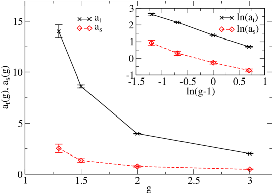
Figure 4: (Color online) Scattering lengths $a_{t}(g)$ and $a_{s}(g)$ as a function of $g$ in units of the lattice constant, $a$. Inset: the logarithms of the scattering lengths as functions of $\ln(g-1)$ show a power law divergence.

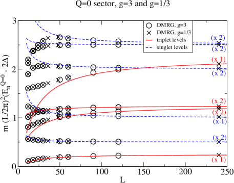
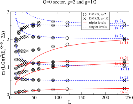
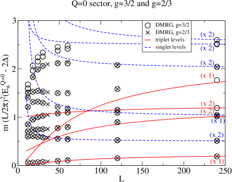
Figure 5: (Color online) Comparison of the rescaled energies from DMRG and the effective theory for $g=3$, $g=2$, and $g=3/2$ in the $Q=0$ sector. The scattering lengths $a_{t}$ and $a_{s}$ were fitted using the lowest lying two levels, respectively. No further fitting for the higher levels was used. Using the duality of the model, we also show the rescaled ferromagnetic spectrum for $\tilde{g}=1/g$ in the $Q=0$ sector.

Although the extrapolations in the case of the scattering lengths are less accurate than in the case of the single-particle parameters, we can now plot the higher energy levels in the $Q=0$ sector using eqns. (13) and (15), and compare them to the appropriately rescaled DMRG data for various system sizes. We find a very good agreement between the numerical results and the predictions for the spectrum of the effective model, as can be seen in fig. 5. A clear convergence to the asymptotic values is observed for large $L$’s, and deviations appear only at smaller system sizes or at higher energy levels, where the asymptotic description must break down.

4.5 Two-particle levels: ferromagnetic phase

As we discussed before, the spectrum on the ferromagnetic side $g<1$ with PBC does not have any single-particle levels, from which we could get the quasiparticle parameters directly. Although, in principle, it would be possible to fit the quasiparticle gap and quasiparticle mass along with the scattering lengths from the two-body spectra given by eqns. (20), this is not needed. As discussed earlier, the duality relation, eq. (3) connects energy scales for $g\leftrightarrow 1/g$, and thus $\Delta(g)$ and $m(g)$ through eq. (27) in both phases. In addition, it also implies that all length scales emerging in the problem must be invariant under the duality transformation $g\leftrightarrow 1/g$: relevant length scales appear in the finite size spectrum as cross-over scales, and by the invariance of the spectrum, they must transform similar to the scattering lengths, eq. (22).

Fig. 5 provides an explicit numerical evidence for the duality relation in the $Q=0$ sector. There we show that the appropriately rescaled DMRG data obtained for $g<1$ completely overlap with the data on the paramagnetic side $g\to 1/g$. This gives a numerical proof for the relations (3), (22), and (27). We emphasize that the duality relation holds for all system sizes $L$.

In addition to the consistency between the effective theory with a reflective asymptotic S-matrix and the numerical data in the $Q=0$ sector, probably the most important check of validity of our assumptions is the comparison to the DMRG results in the ferromagnetic $Q=1$ sector. There the predicted finite size spectrum is given by eqns. (20) together with eq. (23). We emphasize that all parameters of the effective theory are fixed already and no further adjustment to the theoretical spectra is possible. As we show in fig. 6, the effective theory presented here also describes the numerical data in the $Q=1$ sector within numerical precision in the regime, $\xi\ll L$, and fully confirms eqns. (20) and (23). Here $\xi=(mc)^{-1}$ is the correlation length, see also eq. (39).

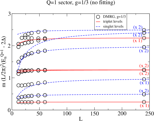
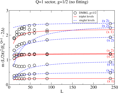
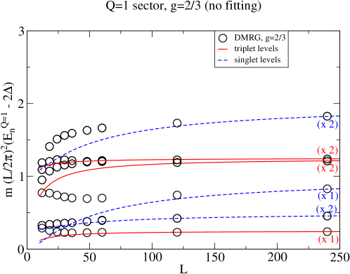
Figure 6: (Color online) The spectra for $g=1/3$, $g=1/2$,$g=2/3$ in the $Q=1$ sector. Only the numerically converged data points and the corresponding curves from the effective theory are shown.

5 Comparison to the scaling Potts field theory

5.1 Scaling Potts field theory as a perturbed conformal field theory

Here we only give a brief review of the scaling Potts field theory; a detailed analysis of the scattering theory is given in a separate paper [20]. The scaling limit of the three-state Potts model at the critical point is a minimal conformal field theory with central charge $C=\frac{4}{5}$ [5, 6]. The Kac table of conformal weights is

$$\left\{h_{r,s}\right\}=\left(\begin{array}[]{ccccc}0&\frac{1}{8}&\frac{2}{3}&\frac{13}{8}&3\\ \frac{2}{5}&\frac{1}{40}&\frac{1}{15}&\frac{21}{40}&\frac{7}{5}\\ \frac{7}{5}&\frac{21}{40}&\frac{1}{15}&\frac{1}{40}&\frac{2}{5}\\ 3&\frac{13}{8}&\frac{2}{3}&\frac{1}{8}&0\end{array}\right)\qquad{r=1,\dots,4;\atop s=1,\dots,5.}$$

The sectors of the Hilbert space are products of the irreducible representations of the left and right moving Virasoro algebras which can be specified by giving their left and right conformal weights as

$$\mathcal{S}_{h,\bar{h}}=\mathcal{V}_{h}\otimes\mathcal{V}_{\bar{h}}\;.$$

There are two possible conformal field theory partition functions for this value of the central charge [9]. The one describing the three-state Potts model is the $D_{4}$ modular invariant, for which the complete Hilbert space is

$$\mathcal{H} = \mathcal{S}_{0,0}\oplus\mathcal{S}_{\frac{2}{5},\frac{2}{5}}\oplus\mathcal{S}_{\frac{7}{5},\frac{7}{5}}\oplus\mathcal{S}_{3,3}$$ (30)

$$\oplus\mathcal{S}_{\frac{1}{15},\frac{1}{15}}^{+}\oplus\mathcal{S}_{\frac{1}{15},\frac{1}{15}}^{-}\oplus\mathcal{S}_{\frac{2}{3},\frac{2}{3}}^{+}\oplus\mathcal{S}_{\frac{2}{3},\frac{2}{3}}^{-}$$

$$\oplus\mathcal{S}_{\frac{2}{5},\frac{7}{5}}\oplus\mathcal{S}_{\frac{7}{5},\frac{2}{5}}\oplus\mathcal{S}_{0,3}\oplus\mathcal{S}_{3,0}\;.$$

Note that not all of the possible representations occur in the Hilbert space; there is another modular invariant partition function called $A_{4}$ which includes all sectors of diagonal form $\mathcal{S}_{h,h}$ allowed by the Kac table exactly once: $\mathcal{H}=\bigoplus_{h}\mathcal{V}_{h}\otimes\mathcal{V}_{h}$. The $A_{4}$ model corresponds to the scaling limit of a higher multicritical Ising class fixed point with symmetry $\mathbb{Z}_{2}$. In contrast, the $D_{4}$ conformal field theory is invariant under the permutation group ${\mathbb{S}}_{3}$ generated by two elements $\mathcal{Z}$ and $\mathcal{C}$ with the relations

$$\mathcal{Z}^{3}=1\;,\qquad\mathcal{C}^{2}=1\;,\qquad\mathcal{CZC}=\mathcal{Z}^{-1}\;,$$

which have the signatures $\mbox{sign }\mathcal{Z}=+1$ and $\mbox{sign }\mathcal{C}=-1$. The sectors in the first line of (30) are invariant under the action of the permutation group, ${\mathbb{S}}_{3}$, while the two pairs on the second line each form two-dimensional irreducible representations, as characterized by the following action of the generators:

$$\mathcal{C}|\pm\rangle=|\mp\rangle\;,\quad\mathcal{Z}|\pm\rangle=\mathrm{e}^{\pm i\Omega}|\pm\rangle\;.$$ (31)

Finally, sectors in the third line of eq. (30) form one-dimensional signature representations, where each element is represented by its signature. These sectors are in one-to-one correspondence with the families of conformal fields: the primary field in the family corresponding to $\mathcal{S}_{h,\bar{h}}$ has left and right conformal weights $h$ and $\bar{h}$, and a corresponding scaling dimension, $\Delta_{h,\bar{h}}=h+\bar{h}$, and is denoted by $\Phi_{h,\bar{h}}$, with an optional upper $\pm$ index for fields forming a doublet of ${{\mathbb{S}}}_{3}$.

Relevant fields are exactly those for which $h+\bar{h}<2$. It is then obvious that the only $\mathbb{Z}_{3}$-invariant spinless relevant field is $\Phi_{\frac{2}{5},\frac{2}{5}}$, which means that the Hamiltonian of the scaling limit of the off-critical three-state Potts model is uniquely determined [6],

$$H=H_{*}+\tau\int dx\;\Phi_{\frac{2}{5},\frac{2}{5}}\;.$$ (32)

The sign of the coupling constant $\tau$ corresponds to the two phases: $\tau>0$ is the paramagnetic, while $\tau<0$ is the ferromagnetic phase. Up to normalization factor, it is given by

$$\tau\propto(g-1)a^{-6/5}\;,$$ (33)

with $a$ the lattice spacing. The scaling limit is achieved by taking $a\rightarrow 0$ and $g\rightarrow g_{c}=1$ such that $\tau$ remains finite. In this limit, the gap

$$\Delta\sim\tau^{5/6}\sim|g-1|^{5/6}\;\hbar c/a$$

remains also finite. Here, for clarity, we restored $\hbar$ and $c$, which are usually both set to unity in relativistic quantum field theory.

The scaling Potts field theory (32) is known to be integrable [15], and its spectrum and scattering matrix was determined exactly [15, 18]. In the paramagnetic phase, the vacuum is non-degenerate and the spectrum consists of a pair of particles $A$ and $\bar{A}$ of mass $m$, which form a doublet under $\mathbb{Z}_{3}$ [17]:

$$\mathcal{C}|A(\beta)\rangle=|\bar{A}(\beta)\rangle\;, \mathcal{Z}|A(\beta)\rangle=\mathrm{e}^{i\Omega}|A(\beta)\rangle\;,$$

$$\mathcal{C}|\bar{A}(\beta)\rangle=|A(\beta)\rangle\;, \mathcal{Z}|\bar{A}(\beta)\rangle=\mathrm{e}^{-i\Omega}|\bar{A}(\beta)\rangle\;.$$ (34)

The excitations $A$ and $\bar{A}$ correspond to the local spin flip excitations of chirality $\sigma=Q=\pm$ of the lattice. The generator $\mathcal{C}$ is identical to charge conjugation ($\bar{A}$ is the antiparticle of $A$). Choosing units in which $\hbar=c=1$, two-dimensional Lorentz invariance implies that the energy and momentum of the particles can be parameterized by the rapidity $\beta$:

$$E=m\cosh\beta,\quad p=m\sinh\beta\;.$$

The two-particle scattering amplitudes are [15]

$$S_{AA}(\beta_{12}) = S_{\bar{A}\bar{A}}(\beta_{12})=\frac{\sinh\left(\frac{\beta_{12}}{2}+\frac{\pi i}{3}\right)}{\sinh\left(\frac{\beta_{12}}{2}-\frac{\pi i}{3}\right)}\;,$$

$$S_{A\bar{A}}(\beta_{12}) = S_{\bar{A}A}(\beta_{12})=-\frac{\sinh\left(\frac{\beta_{12}}{2}+\frac{\pi i}{6}\right)}{\sinh\left(\frac{\beta_{12}}{2}-\frac{\pi i}{6}\right)}\;,$$ (35)

where $\beta_{12}=\beta_{1}-\beta_{2}$ is the rapidity difference of the incoming particles. This $S$ matrix was confirmed by thermodynamic Bethe Ansatz [29]. We remark that the pole in the $S_{AA}=S_{\bar{A}\bar{A}}$ amplitudes at $\beta_{12}=\frac{2\pi i}{3}$ corresponds to the interpretation of the particle $\bar{A}$ as a bound state of two particles $A$, and similarly, $A$ as a bound state of two $\bar{A}$s, under the bootstrap principle (a.k.a. “nuclear democracy”). The pole in $S_{A\bar{A}}=S_{\bar{A}A}$ amplitudes at $\beta_{12}=\frac{\pi i}{3}$ has a similar interpretation in the crossed channel, and it does not correspond to a true bound state in the neutral sector.

The excitations in the ferromagnetic phase are topologically charged [18]. Similar to the lattice model, the vacuum is three-fold degenerate $|0)_{\mu}$ ($\mu=-1,0,1$). The action of ${\mathbb{S}}_{3}$ on the vacua is

$$\mathcal{Z}|0)_{\mu}=|0)_{\mu+1\bmod 3}\;,\qquad\mathcal{C}|0)_{\mu}=|0)_{-\mu}\;,$$

and the excitations are kinks of mass $m$ interpolating between adjacent vacua, and correspond to domain walls on the lattice. The kink of rapidity $\beta$, interpolating from $\mu$ to $\mu^{\prime}$ is denoted by

$$K_{\mu\mu^{\prime}}(\beta)\;,\qquad\mu-\mu^{\prime}=\pm 1\bmod 3\;.$$

The scattering processes of the kinks are of the form

$$K_{\mu\nu}(\beta_{1})+K_{\nu\mu^{\prime}}(\beta_{2})\rightarrow K_{\mu\nu^{\prime}}(\beta_{1})+K_{\nu^{\prime}\mu^{\prime}}(\beta_{2})\;,$$

with the scattering amplitudes equal to

$$S\left(\mu{\nu^{\prime}\atop\nu}\mu^{\prime}\right)(\beta_{12})=\cases{S_{AA}(\beta_{12})\qquad{\rm if}\qquad\nu=\nu^{\prime}\;,\\ S_{A\bar{A}}(\beta_{12})\qquad{\rm if}\qquad\mu=\mu^{\prime}\;.}$$ (36)

This essentially means that, apart from the restriction of kink succession dictated by the vacuum indices (adjacency rules), the following identifications can be made

$$K_{\mu\nu}(\beta)\equiv\cases{A(\beta)\qquad\mu-\nu=+1\bmod 3\;,\\ \bar{A}(\beta)\qquad\mu-\nu=-1\bmod 3\;.}$$ (37)

in all other relevant physical aspects (such as e.g. the bound state interpretation given above).

The validity of the S-matrix expressions (35) and (36) for the scaling Potts model can be checked by comparing the finite size spectrum of the corresponding Bethe Ansatz equations to that of (32) as obtained by the truncated conformal space approach (TCSA). The TCSA was originally developed in [30]. This is performed in detail in [20]. In the TCSA, one determines the finite size spectrum of eq. (32) numerically by truncating the finite volume Hilbert space by imposing an upper cutoff in the eigenvalue of the conformal Hamiltonian. For the ground state, this is equivalent to the standard variational calculus in quantum theory, where the variational wave function Ansatz is expressed as a linear combination of a finite subset of the eigenstates of the conformal Hamiltonian. By looking at the conformal fusion rules implied by the three-point couplings [31, 32, 33], it turns out that the perturbing operator acts separately in the following four sectors:

$$\mathcal{H}_{0} = \mathcal{S}_{0,0}\oplus\mathcal{S}_{\frac{2}{5},\frac{2}{5}}\oplus\mathcal{S}_{\frac{7}{5},\frac{7}{5}}\oplus\mathcal{S}_{3,3}\;,$$

$$\mathcal{H}_{\pm} = \mathcal{S}_{\frac{1}{15},\frac{1}{15}}^{\pm}\oplus\mathcal{S}_{\frac{2}{3},\frac{2}{3}}^{\pm}\;,$$

$$\mathcal{H}_{1} = \mathcal{S}_{\frac{2}{5},\frac{7}{5}}\oplus\mathcal{S}_{\frac{7}{5},\frac{2}{5}}\oplus\mathcal{S}_{0,3}\oplus\mathcal{S}_{3,0}\;,$$ (38)

so the Hamiltonian can be diagonalized separately in each of them. In the lattice language, $\mathcal{H}_{\pm}$ correspond to the sectors $Q=\pm$, while $\mathcal{H}_{0}\oplus\mathcal{H}_{1}$ span the $Q=0$ sector. Charge conjugation $\mathcal{C}$ implies that the Hamiltonian is exactly identical in the sectors $\mathcal{H}_{+}$ and $\mathcal{H}_{-}$. Furthermore, the spectrum is invariant under transformation, $\tau\rightarrow-\tau$ in sectors $\mathcal{H}_{0}$ and $\mathcal{H}_{1}$. This is the consequence of a $\mathbb{Z}_{2}$ symmetry in these sectors, which leaves the fixed point Hamiltonian $H_{*}$ and the conformal fusion rules in these sectors invariant. We remark that the conformal fusion rules do not allow the extension of this symmetry to the $\mathcal{H}_{\pm}$. Away from the critical point, it can be interpreted as the continuum form of the duality transformation (3) in the scaling limit.

As further discussed in  [20], the detailed TCSA calculations indeed confirm that the $S$-matrices (35) and (36) correctly describe the paramagnetic and ferromagnetic phases of the scaling field theory. However, as we discuss below, the Bethe Ansatz spectra computed with (35) and (36) both turn out to be inconsistent with the numerically computed finite size spectra.

5.2 Comparing the scaling field theory to DMRG

In order to compare the DMRG to the scattering matrices (35,36) directly, we need to rescale the variables to appropriate units in which $c=1$. The relativistic relation

$$\Delta=mc^{2}$$

allows to determine the speed of light $c=\sqrt{\Delta/m}$ in lattice units ($aJ/\hbar$). We recall that, according to eq. (4), $\Delta$ is the infinite volume limit of the energy gap between the stationary one-particle state and the ground state, while $m$ can be determined from the large volume behavior of the first excited one-particle state. We then introduce the dimensionless volume variable ($\hbar=1$)

$$l=mcL\;,$$ (39)

i.e. we measure the volume in units of the Compton length. After rescaling the DMRG spectrum to these units, we expect the spectrum of one-particle states to follow the relativistic dispersion,

$$\frac{1}{\Delta}\left(E(L)-E_{0}(L)\right) = \sqrt{1+\left(\frac{p}{mc}\right)^{2}}+O\left(\mathrm{e}^{-\gamma l}\right)\;,$$

$$p/{mc} = {2\pi\;n}/{l}\;,$$

where $E_{0}(L)$ denotes the ground state energy up to exponential finite size corrections. As a side note, we remark that these corrections are due to vacuum polarization and particle self-energy corrections induced by finite volume [34]. The dispersion above indeed describes the numerically obtained finite size spectrum of low energy quasiparticles, as demonstrated in fig. 7. High energy deviations are mainly cut-off effects due to the fact that the DMRG data are not close enough to the fixed point.

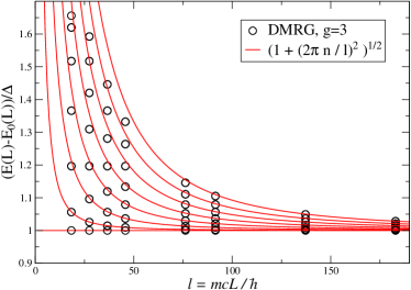
Figure 7: (Color online) Comparing rescaled DMRG data (for $g=3$) to the relativistic one-particle dispersion relation. Length is measured in the Compton length, $l=mcL/\hbar$.

Scaling field theory predicts that (neutral) two-particle states in the paramagnetic phase are described by the Bethe-Yang quantization conditions

$$\mathrm{e}^{il\sinh\beta_{1}}S_{A\bar{A}}(\beta_{1}-\beta_{2})=1\;,\quad\mathrm{e}^{il\sinh\beta_{2}}S_{A\bar{A}}(\beta_{2}-\beta_{1})=1\;,$$

or, in logarithmic form,

$$l\sinh\beta_{1}+2\delta_{A\bar{A}}(\beta_{1}-\beta_{2}) = 2\pi n_{1}\;,$$

$$l\sinh\beta_{2}+2\delta_{A\bar{A}}(\beta_{2}-\beta_{1}) = 2\pi n_{2}\;,$$

with $n_{1}$ and $n_{2}$ integer quantum numbers, and the phase-shift function defined as

$$\delta_{A\bar{A}}(\beta)=-\frac{i}{2}\ln S_{A\bar{A}}(\beta)\;.$$

The Bethe-Yang equations are nothing else than the conditions (11) stated in terms of the notations of the scaling field theory. The energy relative to the ground state can be computed as

$$E(L)-E_{0}(L)=\Delta(\cosh\beta_{1}+\cosh\beta_{2})+O\left(\mathrm{e}^{-\gamma^{\prime}l}\right)\;,$$

and is accurate to all orders in $1/l$, similar to the one-particle states. To conform with the conventions used previously, we plot the rescaled quantity

$$\frac{l^{2}}{(2\pi)^{2}}\;\frac{E(L)-2\Delta-E_{0}(L)}{\Delta}$$

against $l$. The results are shown in fig. 8, which shows that the scaling field theory correctly describes the singlet levels. In the language of the field theory, these are exactly the two-particle levels in the $\mathcal{C}$-odd sector $\mathcal{H}_{1}$. However, the triplet levels cannot be explained by the bootstrap $S$ matrix. In the scaling field theory, these levels are in the $\mathcal{C}$-even sector $\mathcal{H}_{0}$ and are described by the same Bethe-Yang equations, which means that they are exponentially degenerate with their singlet counter-parts. While this picture is fully confirmed by the TCSA analysis [20], it is clearly not consistent with the DMRG spectrum.

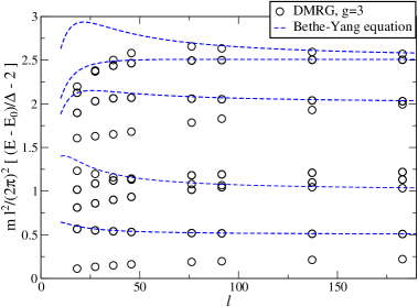
Figure 8: (Color online) Comparison of rescaled DMRG data (for $g=3$) to the two-particle levels predicted by the bootstrap $S$ matrix. While the singlet spectrum is perfectly reproduced without further fitting parameter, the triplet sector cannot be fitted.

To see the problem more clearly, one can perform a direct comparison of the phase-shift function to the DMRG spectrum. Provided the energy levels $E(L)$ are known, the Bethe-Yang equations can be used to extract the phase-shift function from them. The results are shown in fig. 9. For the singlet levels the slope of the phase-shift around the origin agrees quite well with DMRG data, which means that the bootstrap $S$ matrix gives correctly not only the low-energy value of the phase-shift, but also the scattering length. For larger $\beta$ the deviations are explained by cut-off effects since these correspond to lower values of the volume, closer to the scale of the lattice spacing.

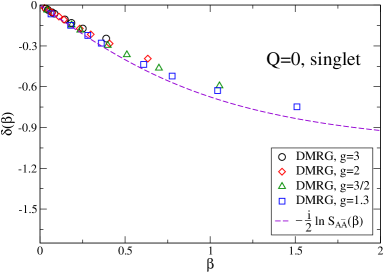
(a)

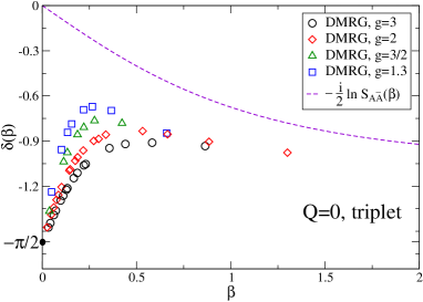
(b)

Figure 9: (Color online) (a) Singlet phase-shift extracted from DMRG and compared to $\delta_{A\bar{A}}$, as a function of rapidity $\beta$. (b) Triplet phase-shift extracted from DMRG and compared to $\delta_{A\bar{A}}$. Dashed lines are the theoretical predictions from the bootstrap.

However, the phase-shift extracted from the triplet states does not agree with the bootstrap prediction at all: neither the low-energy value nor the scattering length is consistent as figure 9 (b) demonstrates. Rather strikingly, however, figure 9 (b) shows evidence for the emergence of a new scale: the slope of the triplet phase shift $\delta_{t}(\beta)$ at $\beta=0$ increases gradually as one approaches $g\to g_{c}=1$, which implies that, in addition to the Compton scale $mc$, yet another small momentum scale $p^{*}<mc$ appears on the lattice. Within the most plausible scenario, this scale could be generated by some irrelevant operator. This would be indeed consistent with the fact that $p^{*}/mc$ appears to vanish as $g\to g_{c}$. Within this scenario, one would also naively expect $\delta_{t}(\beta)$ to scale to the scaling Potts value $\delta_{A\bar{A}}(\beta)$ for any fixed $\beta$ as $g\to g_{c}$. While the $\delta_{t}(\beta)$ curves indeed seem to get somewhat closer to $\delta_{A\bar{A}}(\beta)$ as $g\to g_{c}$, the convergence seems to be extremely slow, and the numerics does not yet give sufficient evidence to conclude.

6 Conclusions

In this work, we determined numerically the two-particle spectrum of the $q=3$ state quantum Potts chain in one dimension, and showed that it is in complete agreement with a simple effective field theory, and a corresponding asymptotic scattering matrix of an exchange form, $S(k\to 0)\to-\hat{X}$. We also showed that the usual scaling Potts field theory does not capture the observed asymptotic behavior and that the bootstrap S matrix reproduces only the ”singlet” part of the finite size spectrum. This, however, does not exclude that the bootstrap S-matrix be valid above some momentum scale, $p^{*}$. Indeed, our data support the emergence of a new small momentum scale on the lattice, $p^{*}<mc$, and it is only below this scale that the asymptotic (exchange) S-matrix dominates. This scale seems to vanish faster than the Compton scale upon approaching the critical point, and above this scale, the collision of quasiparticles is expected to (see below) and may well be described by the scaling Potts model.

Our numerical calculations also allowed us to check the duality between the ferromagnetic and the paramagnetic states. We have shown that in the $Q=0$ sector the whole finite size spectrum obeys duality. As a consequence, the scattering lengths, the quasiparticle masses and gaps also satisfy duality relations, as demonstrated by the numerical analysis of the finite size spectra.

The structure of the asymptotic S-matrix can be understood on simple physical grounds. For interacting massive spinless bosons any local interaction is relevant in one dimension [12], and leads to a scattering phase shift, $\delta=\pm\pi/2$. For particles with some nontrivial internal quantum number the situation is somewhat more subtle. In the antisymmetric (singlet) channel the wave function has a node, and therefore local interactions are asymptotically irrelevant, implying $\delta_{s}(k=0)=0$. In contrast, in the symmetric (triplet) channel the orbital wave function does not vanish when the two particles approach each other. Here interactions are relevant, and lead to $\delta_{t}(k=0)=\pm\pi/2$. These arguments immediately imply an asymptotic S-matrix of the exchange form. To obtain a diagonal S-matrix at $k\to 0$, one would need $\delta_{t}(k=0)=0$, which is only possible for very special effective interactions between the quasiparticles [3], and is not guaranteed by ${\mathbb{S}}_{3}$ symmetry.

Though our lattice calculations are still relatively far away from the critical point itself, it is very hard to believe that the asymptotic theory discussed here would suddenly break down as one approaches the critical point, $g=1$. In this regard, we think that our results are conclusive. However, due to the vanishing of the gap, and the divergence of the correlation length and the scattering lengths, our effective theory will clearly be limited to smaller and smaller momenta, and correspondingly, to smaller and smaller temperatures.

We should also remark that our calculations do not support the existence of bound states in the $\{+-\}$ and $\{-+\}$ channels: every state in the finite size spectrum could be identified as an extended two-particle state. Bound states were also absent in the paramagnetic $Q=\pm$ sectors, where we have just observed extended single particle excitations at and slightly above the gap, $\Delta$, all in agreement with our simple effective theory. We remark that this also agrees with the bootstrap, where particles $A$ and $\bar{A}$ can be interpreted as bound states of $AA$ or ${\bar{A}}{\bar{A}}$ in the spirit of Chew’s “nuclear democracy”; therefore, one does not expect any additional state besides the multi-particle states built from $A$ and $\bar{A}$ (or the corresponding kinks in the ferromagnetic phase).

We believe that the deviations between the scaling Potts field theory and the properties of the quantum Potts chain are rooted at the assumption of integrability. Although the $q=3$ lattice Potts model is integrable at the critical point, $g=1$, it is believed to be non-integrable for other values of $g$. The scaling Potts field theory, on the other hand, is integrable, and the bootstrap, together with the assumption of ${\mathbb{S}}_{3}$ symmetry, leads to a diagonal S-matrix for $q=3$. Similarly, in the perturbed CFT description, one perturbs the continuum Potts model with the leading relevant operator, which leaves the model integrable, and gives a spectrum consistent with the bootstrap S-matrix (as shown in detail by the analysis in [20]). None of the latter methods, at least in their original form, are able to describe the asymptotic ($k\to 0$) properties of the quantum Potts chain for any fixed $g\neq 1$, the reason probably being that requiring integrability conflicts with the true non-integrable nature of the $q=3$ state quantum Potts chain.

We believe that to describe the $q=3$ lattice quantum Potts model, one needs to allow for perturbations or cut-off schemes which violate integrability. In perturbed CFT, a possible candidate would be adding the leading irrelevant operator which already violates integrability. In this case, for any fixed finite rapidity $\beta$ (fixed $k/m(g)c(g)$) one expects to recover the diagonal S-matrix, (35) as $g\to 1$, and a new momentum scale ($p^{*}<mc$) would also be generated, which would then separate the regime described by the scaling Potts model ($|k|\gg p^{*}$) and that described by the asymptotic theory discussed here ($|k|\ll p^{*}$). In fact, our data seem to support this scenario, though unfortunately, we do not have enough numerical evidence to prove or disprove convergence to the scaling Potts S-matrix for $p^{*}<|k|$. While in the singlet sector, shown in fig. 9 (a), the deviation from the bootstrap solution is small for intermediate rapidities $\beta\approx 1$ and can be explained by the finite UV cutoff, the situation is not so clear in the triplet case, shown in fig. 9 (b), where the deviation from the bootstrap prediction remains considerably larger.

The results above need also be discussed in connection to the two-dimensional classical Potts model. The quantum Potts spin chain can be obtained as a Hamiltonian limit of this system, under the assumption that the anisotropy introduced in the Hamiltonian ($\tau$-continuum) limit is irrelevant [35]. We remark that the anisotropy tends to infinity in the Hamiltonian limit as the timelike lattice spacing is taken to zero. There is a number of results obtained by means of the bootstrap S-matrix of the scaling Potts theory which were compared to lattice results in the 2d classical lattice model. In particular, universal amplitude ratios have been calculated from the bootstrap approach [36, 37], and numerical lattice computations as well as low temperature expansions seem to agree with the theoretical predictions [38, 39]. Another such quantity is the so-called static three-quark potential which also agrees with the lattice calculations (on a triangular lattice) [40]. The numerically obtained critical exponents and the central charge of the critical Potts spin chain also agree with the predictions of the scaling Potts model [7]. However, unfortunately, these results cannot be conclusive regarding the structure of the S-matrix: The asymptotic S-matrix governs only a small fraction of the energy eigenstates, and correspondingly, it is expected to have only a very small impact on thermodynamic properties, which provide thus a very indirect way to access the asymptotic properties of the S-matrix. In fact, as shown in Ref. [39], e.g., inclusion of the leading irrelevant operator – possibly responsible for the asymptotic exchange scattering in the quantum Potts chain – in the expansion of the susceptibility has virtually no impact on the value of the ratio $\Gamma_{L}/\Gamma_{T}$ of the longitudinal and transverse susceptibilities. Furthermore, according to our results, for reduced temperatures $|\tau|<0.1$, one would need very large system sizes to observe visible signatures of the asymptotic S-matrix.

Appendix A Duality

We show that a one-to-one correspondence (duality relation) exits between the energies in the $Q=0$ subspace with PBC for couplings $g\leftrightarrow 1/g$. To do this, we introduce two sets of basis states. The first set is defined using the local “spin-flip” states

$$|\{\lambda_{i}\}\rangle\equiv\prod_{i=1}^{L}|\lambda_{i}\rangle_{i}\;,$$ (40)

where each $\lambda_{i}\in\{0,1,-1\}$. Restriction to the $Q=0$ subspace implies $\sum_{i=1}^{L}\lambda_{i}=0$. For a given sequence of $\{\lambda_{i}\}$, there exists another orthogonal set of dual states, defined by using the $\lambda_{i}$ as domain wall labels,

$$|\{\lambda_{i}\}\rangle\rightarrow\widetilde{|\{\lambda_{i}\}\rangle_{\mu}}\equiv\prod_{i=1}^{L}\left|\mu_{i}=\mu+\sum_{j=1}^{i-1}\lambda_{j}\right\rangle_{i}.$$ (41)

By construction, (since $\sum_{i=1}^{L}\lambda_{i}=0$), these states automatically satisfy PBC, but they are not eigenstates of the permutation operator $\mathcal{Z}$. However, we can construct states within the $Q=0$ subspace by defining

$$\widetilde{|\{\lambda_{i}\}\rangle}\equiv\frac{1}{\sqrt{3}}[1+\mathcal{Z}+\mathcal{Z}^{2}]|\{\lambda_{i}\}\rangle_{\mu=1}.$$ (42)

Straightforward algebraic manipulation yields that the matrix elements of the two terms of the Hamiltonian, $H_{1}=\sum_{i}P^{\mu}_{i}P^{\mu}_{i+1}$ and $H_{2}=\sum_{i}P_{i}$ in eq. (1) satisfy the following identities:

$$\widetilde{\langle\{\lambda_{j}\}|}\sum_{i,\mu}P^{\mu}_{i}P^{\mu}_{i+1}\widetilde{|\{\lambda_{j}^{\prime}\}\rangle} = \langle\{\lambda_{j}\}|\sum_{i}P_{i}|\{\lambda_{j}^{\prime}\}\rangle\;,$$

$$\widetilde{\langle\{\lambda_{j}\}|}P_{i}\widetilde{|\{\lambda_{j}^{\prime}\}\rangle} = \langle\{\lambda_{j}\}|\sum_{\mu}P^{\mu}_{i}P^{\mu}_{i+1}|\{\lambda_{j}^{\prime}\}\rangle.$$ (43)

Let us now assume that the states

$$|n\rangle=\sum_{\{\lambda_{j}\}}A^{n}_{\{\lambda_{j}\}}|\{\lambda_{j}\}\rangle$$ (44)

are normalized, orthogonal eigenstates of $H_{1}+gH_{2}$ in the $Q=0$ subspace,

$$\langle m|(H_{1}+gH_{2})|n\rangle=\delta_{nm}E_{n}(g).$$ (45)

Then let us define the set of dual states as

$$\widetilde{|n\rangle}\equiv\sum_{\{\lambda_{j}\}}A^{n}_{\{\lambda_{j}\}}\widetilde{|\{\lambda_{j}\}\rangle}.$$ (46)

Using eq. (43), we immediately see that that these diagonalize the dual Hamiltonian, $H_{1}+1/gH_{2}$,

$$\widetilde{\langle m|}(H_{1}+1/gH_{2})\widetilde{|n\rangle}=(1/g)\langle n|gH_{2}+H_{1}|m\rangle=(1/g)\delta_{nm}E_{n}(g)\;,$$ (47)

yielding the duality relation, eq. (3).

References

References

- [1] Pfeuty P 1970 Ann. Phys. 57 79–90
- [2] Wu F Y 1982 Rev. Mod. Phys. 54 235–268
- [3] Rapp Á and Zaránd G 2006 Phys. Rev. B 74 014433
- [4] Baxter R 1982 Exactly Solved Models in Statistical Mechanics (Academic Press)
- [5] Belavin A A, Polyakov A M and Zamolodchikov A B 1984 Nucl. Phys. B 241 333–380
- [6] Dotsenko V S 1984 Journal of Statistical Physics 34 781–791
- [7] Hamer C J and Barber M N 1981 J. Phys. A 14 2009
- [8] Hamer C J and Batchelor M T 1988 J. Phys. A21 L173
- [9] Cappelli A, Itzykson C and Zuber J B 1987 Nucl. Phys. B 280 445–465
- [10] Haldane F D M 1983 Phys. Lett. A 93 464
- [11] Damle K and Sachdev S 1998 Phys. Rev. B 57, 8307
- [12] Sachdev S 1999 Quantum Phase Transitions (Cambridge: Cambridge University Press)
- [13] Zamolodchikov A B and Zamolodchikov A B 1979 Ann. Phys. 120 253–291
- [14] Köberle R and Swieca J 1979 Phys.Lett. B 86 209
- [15] Zamolodchikov A B 1988 Int. J. Mod. Phys. A 3 743–750
- [16] Tsvelik A M 1988 Nucl. Phys. B 305 675–684
- [17] Smirnov F A 1991 Int. J. Mod. Phys. A 6 1407–1428
- [18] Chim L and Zamolodchikov A 1992 Int. J. Mod. Phys. A 7 5317–5335
- [19] Fendley P and Read N 2002 J. Phys. A 35 10675
- [20] Takács G 2011 Finite volume analysis of the scattering theory in the scaling Potts model Preprint arXiv:1112.5165
- [21] Damle K and Sachdev S 2005 Phys. Rev. Lett. 95 187201
- [22] Rapp Á and Zaránd G 2009 Eur. Phys. J. B 67 7–13
- [23] Sachdev S and Young A P 1997 Phys. Rev. Lett. 78 2220
- [24] Altshuler B L, Konik R M and Tsvelik A M 2006 Nucl. Phys. B 739 311–327
- [25] Mittag L and Stephen M J 1971 J. Math. Phys. 12 441
- [26] Sólyom J 1981 Phys. Rev. B 24 230–243
- [27] White S R 1992 Phys. Rev. Lett 69 2863; White S R 1993 Phys. Rev. B 48 10345
- [28] Calabrese P and Cardy J 2004 J. Stat. Mech. P06002
- [29] Zamolodchikov A B 1990 Nucl. Phys. B 342 695–720
- [30] Yurov V P and Zamolodchikov A B 1990 Int. J. Mod. Phys. A 5 3221–3246
- [31] Fuchs J and Klemm A 1989 Ann. Phys. 194 303
- [32] Petkova V B 1989 Phys. Lett. B 225 357
- [33] Petkova V B and Zuber J B 1995 Nucl. Phys. B 438 347–372
- [34] Lüscher M 1986 Commun. Math. Phys. 104 177
- [35] Sólyom J and Pfeuty P 1981 Phys. Rev. B 24 218–229
- [36] Delfino G and Cardy J L 1998 Nucl. Phys. B 519 551–578
- [37] Delfino G, Barkema G T and Cardy J L 2000 Nucl. Phys. B 565 521–534
- [38] Enting I G and Guttmann A J 2003 Physica B 321 90–107
- [39] Shchur L N, Berche B and Butera P 2002 Nucl. Phys. B 620 579–587; Shchur L N, Berche B and Butera P 2008 Phys. Rev. B 77 144410
- [40] Caselle M, Delfino G, Grinza P, Jahn O and Magnoli N 2006 J. Stat. Mech. P03008