Neutrino processes in partially degenerate neutron matter

Abstract

We investigate neutrino processes for conditions reached in simulations of core-collapse supernovae. Where neutrino-matter interactions play an important role, matter is partially degenerate, and we extend earlier work that addressed the degenerate regime. We derive expressions for the spin structure factor in neutron matter, which is a key quantity required for evaluating rates of neutrino processes. We show that, for essentially all conditions encountered in the post-bounce phase of core-collapse supernovae, it is a very good approximation to calculate the spin relaxation rates in the nondegenerate limit. We calculate spin relaxation rates based on chiral effective field theory interactions and find that they are typically a factor of two smaller than those obtained using the standard one-pion-exchange interaction alone.

1 Introduction

Understanding the mechanisms responsible for supernovae and neutron star formation requires a knowledge of the equation of state and transport mechanisms in matter at densities of the order of that in atomic nuclei and at temperatures ranging up to $10^{11}$K. Despite almost half a century of work on the subject, the question of how a fraction of the large thermal energy from the collapse of the core is transferred to the outer stellar layers, thereby causing a supernova explosion, is one that has yet to find a convincing answer. Because of the high matter density in the new-born protoneutron star, most macroscopic transport processes are ineffective, and a variety of other mechanisms have been considered. These include energy transfer by neutrinos that interact with matter via weak interactions (Colgate & White, 1966; Bethe & Wilson, 1985), magnetic fields in combination with rotation (Ardeljan et al., 2004; Kotake et al., 2006), convection (Herant et al., 1994), or pressure waves and Alfvén waves that may be emitted by the protoneutron star (Burrows et al., 2007; Sagert et al., 2009). Some of these mechanisms lead to very characteristic features in the gravitational wave (Ott, 2009) and neutrino signatures (Dasgupta et al., 2010), and these will be constrained by observations of the next galactic supernova. Other mechanisms have been tested in simulations, which demonstrate that, with current microphysical input, neutrino transport alone is insufficient to generate explosions (Liebendörfer et al., 2001; Rampp et al., 2002; Thompson et al., 2003). However, it is possible to obtain explosions when neutrino heating and fluid instabilities are combined in axisymmetric models of stellar core collapse (Buras et al., 2006; Marek & Janka, 2009; Bruenn et al., 2009; Suwa et al., 2010; Brandt et al., 2011).

In all the above mechanisms, transport by neutrinos is crucial: it is the dominant process for energy emission, it contributes to the transport of energy and lepton number, it influences the radial entropy and lepton fraction gradients that determine the stellar structure and fluid instabilities, and it gives rise to the neutrino luminosities and spectra, which will become the main observables for probing the properties of matter at high density in the next nearby supernova event. Calculations of rates of neutrino processes in dense matter shortly after the discovery of weak neutral currents were reviewed by Freedman et al. (1977). In the early work, the particles participating in the reactions were taken to be free, but, subsequently, effects of strong interactions were taken into account (Sawyer, 1975; Iwamoto & Pethick, 1982). More recently, detailed calculations of rates of neutrino processes have been performed within a mean-field approach (the random phase approximation) by Reddy et al. (1998); Burrows & Sawyer (1998); Reddy et al. (1999); Burrows et al. (2006). One effect not included in these calculations is that excitations can decay due to interactions in the dense medium. As stressed in Raffelt & Seckel (1995); Raffelt et al. (1996); Hannestad & Raffelt (1998), this can lead to an energy transfer in neutrino processes considerably greater than that predicted on the basis of excitations with infinitely long lifetimes (i.e., from recoil effects alone). Lykasov et al. (2005) showed how to include these damping effects in a mean-field approach, and a unified approach to structure factors was described by Lykasov et al. (2008). Detailed calculations were performed based on chiral effective field theory (EFT) interactions in Bacca et al. (2009) for degenerate neutrons. The prime purpose of the present paper is to extend these studies to partially degenerate and nondegenerate conditions.

The plan of the paper is as follows. In Section 2, we analyze the results of simulations of core-collapse supernovae and determine the conditions for which it is important to know rates of neutrino processes. These results point clearly to the need for a better understanding of neutrino properties in regions where nucleons are partially degenerate or nondegenerate. In Section 3, we develop a general formalism based on Landau’s theory of normal Fermi liquids for calculating structure factors of strongly interacting matter. The spin relaxation rate for partially degenerate conditions is derived in Section 4 and the nondegenerate limit is studied in Section 4.1. A key quantity is the spin relaxation rate in partially degenerate neutron matter, and we calculate this in Section 5 based on the one-pion-exchange approximation for nucleon-nucleon interactions, which is the standard one used in simulations (Hannestad & Raffelt, 1998), and from chiral EFT interactions. Particular attention is paid to conditions of importance in supernova simulations. Finally, we summarize and give future perspectives in Section 6.

2 Physical conditions in stellar collapse

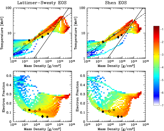
Figure 1: Color-coded plots of the occurrence of thermodynamic conditions during the post-bounce phase of spherically symmetric supernova simulations launched from a $15M_{\odot}$ progenitor star. Left (right) panels refer to a simulation with the Lattimer-Swesty (Shen et al.) equation of state (EOS). Upper (lower) panels show temperature $T$ (electron fraction $Y_{e}$) versus mass density $\rho$. The occurrence is expressed on a logarithmic scale by the amount of matter which experiences a specific set of conditions, normalized to $M_{\odot}$, integrated over time during the post-bounce phase [see text and Equation (1) for details]. The solid lines indicate where the temperature is equal to the Fermi temperature of the baryons, $T_{\rm F}=(3\pi^{2}\rho/m)^{2/3}/2m$, and the dashed lines represent the conditions specified by Equation (2). In each panel, six different symbols indicate the conditions under which neutrinos decouple thermally from matter. Squares refer to $\nu_{e}$, diamonds to $\bar{\nu}_{e}$, and stars to $\nu_{\mu,\tau}$ and $\bar{\nu}_{\mu,\tau}$. Unfilled symbols refer to the early post-bounce phase ($\approx 50\,{\rm ms}$ after bounce), whereas filled symbols refer to the latest times considered ($\approx 400\,{\rm ms}$ after bounce for the Lattimer-Swesty EOS simulation and $\approx 430\,{\rm ms}$ after bounce for the Shen et al. case).

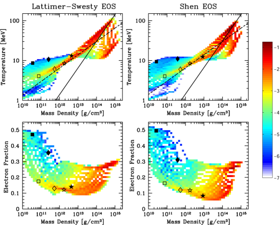
Figure 2: Same as Figure 1, but for a $40M_{\odot}$ progenitor. As in Figure 1, unfilled symbols refer to the early post-bounce phase ($\approx 50\,{\rm ms}$ after bounce), whereas filled symbols refer to the latest times considered, which is close to black-hole formation ($\approx 430\,{\rm ms}$ after bounce for the Lattimer-Swesty EOS simulation and $\approx 1.36\,{\rm s}$ after bounce for the Shen et al. case).

We consider the results of numerical simulations of the collapse of $15M_{\odot}$ and $40M_{\odot}$ stars in a spherically symmetric supernova model with Boltzmann neutrino transport (Fischer et al., 2009). Figure 1 shows an overview of the conditions that are reached after the collapse of the stellar core of a $15M_{\odot}$ progenitor star. The upper panels are constructed from a two-dimensional histogram in the parameter space spanned by the matter density $\rho$ and the matter temperature $T$. The color of each bin $[\rho_{i},\rho_{i+1}]$, $[T_{j},T_{j+1}]$ is chosen according to the value of a time- and mass-weighted measure of the occurrence of the conditions corresponding to the bin, where the labels on the color bar specify the value of

$$H(\rho,T)=\log_{10}\biggl{[}\frac{1}{\tau M_{\odot}}\int_{0}^{\tau}dt\int_{0}^{M}dM_{\rm encl}\>\chi_{ij}(t,M_{\rm encl})\biggr{]}\,,$$ (1)

where $\chi_{ij}(t,M_{\rm encl})=1$ if the density and temperature are reached in the bin, $\rho_{i}\leqslant\rho(t,M_{\rm encl})<\rho_{i+1}$ and $T_{j}\leqslant T(t,M_{\rm encl})<T_{j+1}$, and $\chi_{ij}(t,M_{\rm encl})=0$ otherwise. The integral over time $t$ runs from zero (at the time of core bounce) to the final time $\tau$, while the integration over the enclosed mass $M_{\rm encl}(R)=\int_{0}^{R}dr\,4\pi r^{2}\rho(r)$ runs from zero at the center of the star to the total mass $M$ considered in the computational domain. Hence, a white bin in the $\rho$–$T$-plane indicates that the corresponding conditions rarely occur in the simulation, while a red bin indicates conditions occurring for a large mass and/or for a long time duration. The lower panels are constructed in the same way, but with the temperature in Equation (1) replaced by the electron fraction $Y_{e}$. The symbols indicate where neutrinos decouple from matter. This was determined by comparing the mean neutrino energy in the simulation with the mean neutrino energy expected for neutrinos in equilibrium at the temperature of the matter. The symbols mark the conditions under which the difference between the two mean energies was equal to $5\%$.

Figure 2 shows the conditions for a simulation that was launched from a more massive progenitor star with a main sequence mass of $40M_{\odot}$. All panels show on the far right-hand side the cold core of the protoneutron star at densities around $3\times 10^{14}\,\text{g}\,\text{cm}^{-3}$, temperatures around $10-20\,\text{MeV}$ and an electron fraction just below $Y_{e}=0.3$. The black solid line shows the baryon Fermi temperature as a function of density (see caption) and thus the neutrons in this regime are degenerate. This matter lies in the inner part of the stellar core, which is collapsing subsonically, and it is unaffected by the bounce shock that forms outside the core at the sonic point and runs outward. The compactness of this highest density regime is sensitive to the equation of state (EOS) of neutron-rich matter. In parametric EOSs, this depends mainly on the incompressibility and the symmetry energy. If the EOS is stiff, the mantle of the protoneutron star will lie at a larger radius in a lower gravitational potential. This leads to comparatively small neutrino luminosities and soft spectra. If the EOS is soft, the core of the protoneutron star will be more compact and the mantle will lie at a smaller radius deep in the gravitational potential. This leads to larger neutrino luminosities and harder spectra. This general relationship between neutrino emission and proto-neutron star size applies to all factors that influence the compactness of the core: general relativistic effects (Liebendörfer et al., 2001; Bruenn et al., 2001), different progenitor masses (Liebendörfer et al., 2003), and different EOSs (Sumiyoshi et al., 2007). In the left panels of Figures 1 and 2, we show results from simulations based on the Lattimer-Swesty EOS (Lattimer & Swesty, 1991), which produces a more compact protoneutron star core, while the right panels show results from a simulation with the stiffer Shen et al. (1998) EOS. New constraints from neutron matter calculations (Hebeler et al., 2010) and from modeling X-ray burst sources (Steiner et al., 2010) favor EOSs that yield more compact (cold) neutron stars than the Shen et al. (1998) EOS can give.

When the bounce shock runs through the mantle of the protoneutron star, it causes a temperature jump. Hence, in the upper panels of Figures 1 and 2, matter in the cold core is well separated from that in the shock-heated mantle, which is found above the black line that indicates partially degenerate conditions. The conditions in the mantle are represented by a rather narrow band in the $\rho$–$T$-plane that runs from densities around $10^{14}\,\text{g}\,\text{cm}^{-3}$ at temperatures of $\sim 30\,\text{MeV}$ down to densities of $10^{11}\,\text{g}\,\text{cm}^{-3}$ at temperatures of $\sim 3\,\text{MeV}$. This band is approximately described by the relation

$$T=3\,\biggl{(}\frac{\rho}{10^{11}\,\text{g}\,\text{cm}^{-3}}\biggr{)}^{1/3}{\rm MeV}\,,$$ (2)

for which the temperature at $\rho=10^{14}\,\text{g}\,\text{cm}^{-3}$ is equal to the Fermi temperature at that density. In Figures 1 and 2, this relation is shown as dashed lines. This behavior may be understood as being a consequence of the fact that the shocked matter expands approximately adiabatically (neglecting neutrino heating). Due to the high temperature, most of the entropy resides in the leptons and the photons, which behave as ideal, relativistic gases, for which the entropy per unit volume varies as $T^{3}$. Since the baryon density is proportional to $\rho$, the temperature on adiabats behaves approximately as $T\sim\rho^{1/3}$. Note that the maximum temperature depends strongly on the mass of the progenitor star and, in the case of the $15M_{\odot}$ model, also on the EOS. During the first second of the post-bounce phase, more than $70\%$ of the $\nu_{e}$, $\bar{\nu}_{e}$ and $\nu_{\mu,\tau}$ luminosities are emitted from this hot mantle of the protoneutron star. At higher densities, the influence of the neutrinos on the supernova dynamics is comparatively small, because neutrinos are trapped so that thermal and weak equilibrium with the matter is established. At very low densities, the influence of neutrino processes is limited by small weak-interaction rates. The sizable electron chemical potential in the mantle favors electron capture over positron capture, so that it is the neutrino emitting protoneutron star mantle that deleptonizes most efficiently and becomes the most neutron-rich region in the computational domain. The resulting low electron fractions in the density interval $\rho=10^{11}\,\text{g}\,\text{cm}^{-3}$ to $10^{14}\,\text{g}\,\text{cm}^{-3}$ can be seen in the lower panels of Figures 1 and 2.

Neutrino reaction rates exhibit a strong energy dependence; as a consequence, neutrinos with different energies decouple from the matter at different locations. As an approximate measure of where decoupling occurs, we take the radius at which the mean neutrino energy obtained from the simulation begins to differ from the one expected for a gas of neutrinos in thermal equilibrium with the matter. The symbols in Figures 1 and 2 indicate the thermodynamic conditions at these points. To indicate the time evolution, the conditions for decoupling are shown at $50\,{\rm ms}$ after bounce (open symbols) and at the end of the simulation (filled symbols). In general, the neutrinospheres for electron neutrinos (square symbols) are found at the lowest density due to their charged-current reactions with neutrons, which are the most abundant species under the given conditions. Electron antineutrinos, which have charged-current reactions with protons in addition to neutral-current reactions, decouple on average at densities ten times larger (diamonds). The $\mu$ and $\tau$ neutrinos and antineutrinos interact with matter only via neutral-current reactions and therefore decouple at the highest density, as indicated by the stars. This density hierarchy translates into a temperature hierarchy for the regions from which neutrinos are emitted. As a result, the spectra of $\nu_{\mu,\tau}$ and $\bar{\nu}_{\mu,\tau}$ are harder than that of $\bar{\nu}_{e}$, which in turn is harder than that of $\nu_{e}$.

The post-bounce evolution can be separated into two phases. During the first phase the mass of the protoneutron star is significantly lower than the maximum mass supported by the EOS. Thus, the protoneutron star does not contract significantly and the neutrinospheres move to higher density with time as the accretion rate and the density of the accreting layers decrease. Because regions at higher density have higher temperature, this also leads to a continuous increase of the temperature of emitted neutrinos. However, in spherically symmetric models it can happen that the steady cooling by $\nu_{\mu,\tau}$ and $\bar{\nu}_{\mu,\tau}$ emission within a narrow range of the mass coordinate decreases the local temperature sufficiently that the mean energy of $\nu_{\mu,\tau}$ and $\bar{\nu}_{\mu,\tau}$ decreases and eventually falls below that of the $\bar{\nu}_{e}$ (Liebendörfer et al., 2004). The first phase of the post-bounce evolution is well represented by the $15M_{\odot}$ model shown in Figure 1. After the onset of the supernova explosion, which was not successful for the models shown in Figures 1 and 2, the mean energies of the neutrino spectra decrease as the protoneutron star cools (Fischer et al., 2009). Due to the lower opacity for neutrinos with lower energy, the neutrinospheres continue to shift to higher density and make the high-density part of the protoneutron star more ‘neutrino-visible’.

The first phase of the postbounce evolution dictates the success of the supernova explosion, i.e., whether sufficient entropy can be accumulated behind the standing accretion shock to revive it and drive it through the outer layers of the star. This phase of the supernova mechanism is extremely challenging to model because the emission, transport and absorption of neutrinos behind the shock couples to vigorous three-dimensional fluid instabilities between the neutrinospheres and the accretion shock. These multidimensional effects are not included in the data shown in Figures 1 and 2.

If an explosion has not taken place during the first stage, the post-bounce evolution enters a second phase when the mass of the protoneutron star approaches the maximum stable mass. This scenario may occur in the rarer cases of ‘failed supernovae’ that are triggered by the collapse of a very massive progenitor star. As the limiting stable mass of the protoneutron star is approached, accretion makes the protoneutron star more compact and pushes matter with high entropy into the regime of the neutrinospheres. The corresponding temperature change increases the opacity so that the neutrinospheres shift to lower densities, as can be seen in Figure 2. This leads to a dramatic increase in the mean energy of emitted $\nu_{\mu,\tau}$ and $\bar{\nu}_{\mu,\tau}$ (Liebendörfer et al., 2004; Sumiyoshi et al., 2007). However, only the $40M_{\odot}$ model reaches this second phase within the duration of the simulation. With the Lattimer-Swesty EOS, it takes $0.43\,{\rm s}$ to form a black hole, while for the stiffer Shen et al. EOS it takes $1.4\,{\rm s}$ (Sumiyoshi et al., 2007; Fischer et al., 2009).

In summary, the emission of neutrinos from the partially degenerate hot mantle of the protoneutron star, the EOS at nuclear densities, and the accretion rate set by the progress of the supernova shock and the density of the outer layers of the progenitor star are the key ingredients that determine the compactification of the protoneutron star during the early post-bounce evolution. The emission of neutrinos also shapes the radial entropy and lepton number profiles that determine where stratified layers of matter are stable against convection. The emitted neutrinos finally can be absorbed by matter at larger radii between the protoneutron star mantle and the standing accretion shock. The heat transferred per absorbed neutrino increases with the difference between the temperature of the neutrinos and that of the absorbing matter. This difference increases with the distance from the neutrinospheres, but the neutrino number flux decreases with the distance because of geometrical dilution. Hence, there is a region close to the protoneutron star where heating is most effective. This peak heating at the base of the matter lying between the protoneutron star and the standing accretion shock establishes a negative entropy gradient. The entropy gradient induces fluid instabilities that start to transport energy to the shock by mechanical turnover (Herant et al., 1994; Marek & Janka, 2009). The perturbations in the convective fluid flow are enhanced by the standing accretion shock instability (Blondin et al., 2003; Foglizzo et al., 2007). The fluid instabilities and the net rate of neutrino cooling and heating determine the further evolution and geometry of the supernova. It is therefore essential for supernova models to accurately treat the neutrino-matter interactions in the hot mantle of the protoneutron star under the conditions shown in Figures 1 and 2, which we shall investigate in Section 5.

3 General formalism

Motivated by the relevant supernova conditions, we extend our work on neutrino processes in degenerate matter (Lykasov et al., 2008; Bacca et al., 2009) to the case of partially degenerate and nondegenerate neutrons.

The basic ingredients in the calculation of rates of neutrino processes are the structure factors for the vector and axial vector response (Raffelt, 1996). For nonrelativistic neutrons, the vector current couples to the neutron density and the axial current to the neutron spin. We denote the coupling strengths by $C_{V}$ and $C_{A}$, respectively, and for free neutrons $C_{V}=−1/2$ and $C_{A}=−g_{A}/2=−1.26/2$. We shall focus on the axial current response for two reasons. The first is that it is responsible for the largest contributions to rates of neutrino processes. The second is that axial current processes have potential for equilibrating neutrino energy distributions because the axial current is not conserved and therefore it is possible for the energy transfer to or from the neutrinos to be nonzero even for processes in which there is a small momentum transfer. For the vector interaction, the energy transfer vanishes for zero momentum transfer because the vector current is conserved. For neutrons, the structure factor for the axial current therefore has the form

$$S_{\rm A}(\omega,{\bf q})=C_{A}^{2}\,S_{\sigma}(\omega,{\bf q})\,,$$ (3)

where the spin structure factor is given by

$$S_{\sigma}(\omega,{\bf q})=\frac{1}{\pi n}\,\frac{1}{1-{\rm e}^{-\omega/T}}\,{\rm Im}\,\chi_{\sigma}(\omega,{\bf q})\,.$$ (4)

Here $\chi_{\sigma}$ is the spin-density–spin-density response function. (We use units in which $\hbar=c=k_{\rm B}=1$.)

We begin by presenting a phenomenological approach. As has been stressed by Raffelt and coworkers, it is a good first approximation in many situations to consider the long-wavelength response because the momentum transfer to the nucleons is of the order of a typical neutrino momentum, which is generally small compared with the characteristic momentum of a nucleon. The latter is of the order of the Fermi momentum $(3\pi^{2}n)^{1/3}$ for degenerate matter and the thermal momentum $(mT)^{1/2}$, where $m$ is the nucleon mass, for nondegenerate matter. We consider the relaxation of $S$, the total $z$-component of the spin of the system to its equilibrium value $S_{\rm eq}$, which is given in linear response theory by

$$S_{\rm eq}=-\chi_{M}\,U_{z}\,,$$ (5)

where $-U_{z}$ corresponds to the strength of a magnetic field that polarizes the system and $\chi_{M}$ is, apart from factors, the static magnetic susceptibility. If one assumes that the approach of $S$ to its equilibrium value is proportional to the difference between $S$ and its equilibrium value, we may write

$$\frac{dS}{dt}=-\frac{S-S_{\rm eq}}{\tau}\,,$$ (6)

where $\tau$ is a characteristic relaxation time. The quantity $1/\tau$ corresponds to what Hannestad & Raffelt (1998) refer to as the spin fluctuation rate. The total spin of the system thus approaches its equilibrium value exponentially, if the magnetic field does not depend on time.

On Fourier transforming Equations (5) and (6) one finds for the frequency-dependent response function

$$\chi_{\sigma}(\omega)\equiv-\frac{S}{U_{z}}=\frac{\chi_{M}}{1-{\rm i}\omega\tau}\,.$$ (7)

In order to make detailed calculations, we shall consider nucleonic matter as a system of interacting quasiparticles. We shall assume that the spectrum of a single quasiparticle may be described by an effective mass $m^{*}$ that is independent of its momentum ${\bf p}$, and therefore the energy of a single quasiparticle is given by

$$\epsilon_{{\bf p}\sigma}=\epsilon_{0}+\frac{p^{2}}{2m^{*}}\,.$$ (8)

We take into account two-body quasiparticle interactions, with a spin-dependent part of the form

$$f_{{\bf p}{\bm{\sigma}}_{1},{\bf p}^{\prime}{\bm{\sigma}}_{2}}=g_{0}\,{\bm{\sigma}}_{1}\cdot{\bm{\sigma}}_{2}\,,$$ (9)

where ${\bm{\sigma}}_{i}$ are Pauli matrices. The theory may be regarded as an extension of Landau’s theory of Fermi liquids generalized to higher temperatures when the quasiparticle interaction is independent of the momenta of the quasiparticles. The parameters $m^{*}$ and $g_{0}$ generally depend on temperature and density, and their values are chosen to ensure that bulk properties such as the specific heat and magnetic susceptibility agree with the results of more microscopic calculations.

We shall take the coupling of the spin to the external field $U_{z}$ to be given by a change in the energy of a quasiparticle, $\epsilon_{{\bf p}\sigma}$, equal to

$$\delta\epsilon_{{\bf p}\sigma}=\sigma\,U_{z}\,.$$ (10)

By generalizing the standard calculation of the static magnetic susceptibility (Baym & Pethick, 1991) to higher temperatures, one finds

$$\chi_{M}=\frac{\chi^{0}}{1+g_{0}\chi^{0}}\,,$$ (11)

where

$$\chi^{0}=-\sum_{{\bf p}\sigma}\frac{\partial n(\epsilon_{{\bf p}\sigma})}{\partial\epsilon_{{\bf p}\sigma}}\,,$$ (12)

is the static susceptibility in the absence of interactions between quasiparticles and

$$n(\epsilon)=\frac{1}{{\rm e}^{(\epsilon-\mu)/T}+1}\,,$$ (13)

is the Fermi function, $\mu$ being the chemical potential. At temperatures low compared with the Fermi degeneracy temperature $T_{\rm F}=p_{\rm F}^{2}/2m^{*}$, where $p_{\rm F}$ is the Fermi momentum, the density of states $\chi^{0}=m^{*}p_{\rm F}/\pi^{2}$ for a single species of particles with two spin states, while at temperatures high compared with $T_{\rm F}$, one finds the Curie law $\chi^{0}=n/T$. On inserting Equation (12) into Equation (7) one finds

$$\chi_{\sigma}(\omega)=\frac{\chi^{0}}{1+g_{0}\chi^{0}-{\rm i}\omega\tau_{\sigma}}\,,$$ (14)

where

$$\tau_{\sigma}=\tau\,(1+g_{0}\chi^{0})\,.$$ (15)

This equation has the same form as in Lykasov et al. (2008) [see, e.g., Equation (24)]. The significance of the time $\tau_{\sigma}$ may be brought out by writing Equation (6) in terms of the deviation of the spin from its local equilibrium (l.e.) value

$$S_{\rm l.e.}=\chi^{0}(-U_{z}+g_{0}\,S)\,,$$ (16)

which is the equilibrium spin density in a system exposed to an external field $-U_{z}$ plus a “molecular field” $g_{0}\,S$ due to interactions with the other particles. Equation (6) then becomes

$$\frac{dS}{dt}=-\frac{S-S_{\rm l.e.}}{\tau_{\sigma}}\,.$$ (17)

From kinetic theory, one saw in the degenerate limit how mean-field effects enter relaxation rates (Lykasov et al., 2008): the time $\tau_{\sigma}$ does not depend on mean-field effects, while the characteristic time for relaxation of a deviation of the total spin from its equilibrium value is decreased by the factor by which mean-field effects decrease the magnetic susceptibility. The reason for this effect is that when the magnetic susceptibility is reduced, the free energy difference driving the return to equilibrium, which for a given spin deviation is inversely proportional to the magnetic susceptibility, is increased, and relaxation is faster.

In the work of Hannestad & Raffelt (1998), the normalization of the spin response function was determined by the condition that it give correctly the static structure factor, which was assumed to be that of a noninteracting gas. It is therefore of interest to investigate the relationship between the static structure factor and the spin response function when interactions are taken into account. The static structure factor $S_{\sigma}({\bf q})$ is defined by

$$S_{\sigma}({\bf q})=\int_{-\infty}^{\infty}d\omega\,S_{\sigma}(\omega,{\bf q})\,.$$ (18)

Since the dynamical structure factor $S(\omega,{\bf q})$ is related to the response function by Equation (4), one has

$$S_{\sigma}({\bf q})=\frac{1}{n}\int_{-\infty}^{\infty}\frac{d\omega}{\pi}\,\frac{{\rm Im}\chi_{\sigma}(\omega,{\bf q})}{1-{\rm e}^{-\omega/T}}=\frac{1}{n}\int_{-\infty}^{\infty}\frac{d\omega}{2\pi}\,{\rm Im}\chi_{\sigma}(\omega,{\bf q})\,\coth[\omega/(2T)]\,,$$ (19)

where we have used the fact that ${\rm Im}\chi_{\sigma}(\omega,{\bf q})$ is an odd function of $\omega$. From the inequality $\bigl{|}\coth[\omega/(2T)]\bigr{|}\geqslant|2T/\omega|$, it follows that

$$S_{\sigma}({\bf q})\geqslant\frac{T}{n}\int_{-\infty}^{\infty}\frac{d\omega}{\pi}\,\frac{{\rm Im}\chi_{\sigma}(\omega,{\bf q})}{\omega}=\frac{T}{n}\,\chi_{M}\,,$$ (20)

the equality applying only if all the weight of ${\rm Im}\chi_{\sigma}$ is at zero frequency. Using Equation (14) for the response function, one finds

$$S_{\sigma}({\bf q}\rightarrow 0)\geqslant\frac{T}{n}\,\frac{\chi^{0}}{1+g_{0}\chi^{0}}\,.$$ (21)

These results represent a generalization of Equation (15) of Hannestad & Raffelt (1998) to allow for spin correlations. For neutron matter at low temperature, $g_{0}\chi^{0}$ is equal to the Landau parameter $G_{0}$, which is calculated to be approximately 0.45 at a density of $\rho_{0}/100$ and 0.8 at nuclear saturation density, $\rho_{0}=2.8\times 10^{14}\,\text{g}\,\text{cm}^{-3}$ (Schwenk et al., 2003), and therefore interactions depress the static structure factor by up to almost a factor of two. For density correlations, the equality sign applies in the long-wavelength limit, since total particle number is conserved and, consequently, matrix elements of the density operator to states with nonzero excitation energy vanish in this limit (Baym & Pethick, 1991, Section 1.3.3). If interactions that do not conserve spin are neglected, the inequality (20) becomes an equality at long wavelengths. This approximation has been employed in calculations of neutrino processes in nondegenerate matter at low densities based on the virial expansion (Horowitz & Schwenk, 2006).

A number of cautionary remarks about our approach should be made. First, in the above we have calculated only the contribution to the susceptibility due to the coupling of the external field to single quasiparticle-quasihole intermediate states. The effects of multipair states are taken into account in so far as they may be regarded as arising from single-pair states as a consequence of the collision term in the kinetic equation. Other processes that can result in the creation of two- and higher-quasiparticle-quasihole states, e.g., two-body contributions to effective operators (Menendez et al., 2011), have been neglected. As emphasized in Olsson et al. (2004), because of the noncentral character of nuclear forces, these are nonzero even for very long wavelengths of the exciting field. Similarly, we have neglected many-body contributions that can renormalize the magnetic moment (or in the case of the coupling to the weak field, the weak charge) of the nucleon. In estimating rates of processes one must multiply the above results by the square of the appropriate renormalization factors.

One may ask how good is the assumption of a single relaxation time. This question was addressed for degenerate nucleons in Pethick & Schwenk (2009). There it was shown for $\omega\ll T$ that, if the relaxation time is chosen to reproduce the leading behavior for $\omega\gg 1/\tau_{\sigma}$, the real and imaginary parts of the response function given by Equation (14) differ from the result obtained by solving the transport equation exactly by less than 10%. For nondegenerate matter this question has not yet been addressed, but one can draw on experience with other transport problems for this case. The relaxation time at high values of $\omega\tau_{\sigma}$ is given by the simplest variational estimate for the relaxation time, which uses a trial function proportional to the quasiparticle spin. The actual relaxation time at low frequencies is longer than this estimate, but to date no estimates of it have been made. For nondegenerate, spinless atomic gases one finds that relaxation times for viscosity and thermal conduction in the hydrodynamic regime differ from the simplest variational estimates by amounts that are typically of order two per cent or less (Chapman & Cowling, 1970). The part of the interaction relevant for spin relaxation depends on the spin of the particles, and it has a different spatial dependence from typical interactions between spinless atoms, so it is desirable to calculate the ratio of the relaxation times in the hydrodynamic and collisionless regimes for nuclear interactions. However, it seems unlikely that the deviations will be more than a few per cent, which is small compared with the uncertainties in the strong scattering amplitudes that enter the relaxation rates. For practical purposes it is therefore expected to be a very good approximation to use Equation (14) for all $\omega\tau_{\sigma}$.

4 Relaxation time

In this section, we calculate the response function microscopically for frequencies high compared to the collision rate. In terms of the phenomenological model discussed in the previous section, this is given by

$$\chi(\omega)\simeq{\rm i}\,\frac{\chi^{0}}{\omega\tau_{\sigma}}\,.$$ (22)

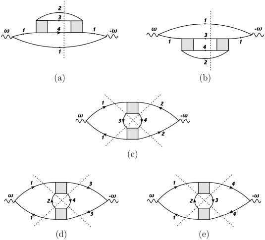
Figure 3: Diagrams for the imaginary part of the response function. Solid lines represent quasiparticle propagators and the square boxes interactions of quasiparticles. The dashed lines represent two-quasiparticle–two-quasihole states that are on the energy shell.

Quantitatively, the response function may be calculated using field-theoretical methods, as described in Lykasov et al. (2005). The contribution to the response function proportional to $1/\omega$ follows from the diagrams shown in Figure 3. In the figure, the lines represent quasiparticles, and the interaction vertices are those for quasiparticles. The square boxes denote scattering vertices for quasiparticles, symmetrized with respect to the incoming and outgoing states. The diagrams in Figure 3 (a) correspond to self-energy corrections which take into account the nonzero width of the quasiparticles, while those in Figure 3 (b)–(d) correspond to vertex corrections.

As we have argued above, the leading contribution to the response functions at large $\omega$ is imaginary, and a convenient way of calculating this is by use of the techniques developed in field theory (Landau, 1959; Cutkosky, 1960; Taylor, 1960), which have been exploited in the context of condensed matter in Langer (1961, 1962) and Carneiro & Pethick (1975). The energy denominators that lead to singularities may be identified by finding intermediate states in the response function which have the property that when lines corresponding to the intermediate state are cut, the diagram falls into just two parts. In Figure 3 such intermediate states corresponding to two-quasiparticle–two-quasihole states are denoted by dashed lines. By including all such intermediate states one automatically includes contributions that correspond both to “in-scattering” and “out-scattering” terms in an approach based on a kinetic equation. On evaluating the response function one finds

$$\chi(\omega) ={\rm i}\,\frac{2\pi}{\omega^{2}}\,\frac{1}{2}\,\sum_{1234}\sigma_{1}(\sigma_{1}+\sigma_{2}-\sigma_{3}-\sigma_{4})$$

$$\quad\times\Bigl{[}\bigl{|}\langle 34|{\cal T}|12\rangle\bigr{|}^{2}n_{1}n_{2}(1-n_{3})(1-n_{4})-\bigl{|}\langle 12|{\cal T}|34\rangle\bigr{|}^{2}(1-n_{1})(1-n_{2})n_{3}n_{4})\Bigr{]}\delta^{+}_{\epsilon}\delta_{\bf p}\,.$$ (23)

Here the index 1 is shorthand for ${\bf p}_{1}\sigma_{1}$ and so on, $n_{i}$ are equilibrium distribution functions, $\delta_{\bf p}\equiv\delta({\bf p}_{1}+{\bf p}_{2}-{\bf p}_{3}-{\bf p}_{4})$ and $\delta^{\pm}_{\epsilon}\equiv\delta(\pm\omega+\epsilon_{1}+\epsilon_{2}-\epsilon_{3}-\epsilon_{4})$, and we have dropped the momentum transfer ${\bf q}$ from the momentum conservation condition according to the arguments given above. The factor of $1/2$ is to avoid double counting of final states when the sums over ${\bf p}_{3}$ and ${\bf p}_{4}$ are unrestricted. The two different scattering matrices in Equation (23) may be combined if one makes use of the fact that the interaction is invariant under time reversal, which implies

$$\langle 34|{\cal T}|12\rangle=\langle-1,-2|{\cal T}|-3,-4\rangle^{*}\,,$$ (24)

where the minus sign indicates that both the momentum of a quasiparticle and its spin must be reversed. Since the distribution function depends on momentum only through its magnitude, since all momenta are summed over, and since each term is quadratic in the spins of quasiparticles, it follows that $\chi(\omega)$ has the form of Equation (22) with

$$\frac{1}{\tau_{\sigma}}=\frac{\pi}{\chi^{0}\,\omega}\,\sum_{1234}\sigma_{1}(\sigma_{1}-\sigma_{2}-\sigma_{3}-\sigma_{4})\bigl{|}\langle 34|{\cal T}|12\rangle\bigr{|}^{2}\,n_{1}n_{2}(1-n_{3})(1-n_{4})\,\delta_{\bf p}\,\bigl{[}\delta^{+}_{\epsilon}-\delta^{-}_{\epsilon}\bigr{]}\,.$$ (25)

This form demonstrates explicitly the fact that the relaxation time is an even function of $\omega$, as is required by the condition that the real part of $\chi$ be an even function of $\omega$ and the imaginary part an odd function. By making use of the relation

$$\frac{n_{i}}{1-n_{i}}={\rm e}^{-(\epsilon_{i}-\mu)/T}\,,$$ (26)

and exchanging the roles of 1 and 2 with 3 and 4 in the sum in Equation (25), one can see that the second term is ${\rm e}^{-\omega/T}$ times the first one, and therefore

$$\frac{1}{\tau_{\sigma}}=\frac{(1-{\rm e}^{-\omega/T})}{\omega}\,\frac{\pi}{\chi^{0}}\,\sum_{1234}\sigma_{1}(\sigma_{1}+\sigma_{2}-\sigma_{3}-\sigma_{4})\bigl{|}\langle 34|{\cal T}|12\rangle\bigr{|}^{2}\,n_{1}n_{2}(1-n_{3})(1-n_{4})\,\delta_{\bf p}\,\delta^{+}_{\epsilon}\,.$$ (27)

This may be expressed in the more symmetrical form

$$\frac{1}{\tau_{\sigma}}=\frac{2\sinh[\omega/(2T)]}{\omega}\,\frac{\pi}{\chi^{0}}\,\sum_{1234}\sigma_{1}(\sigma_{1}+\sigma_{2}-\sigma_{3}-\sigma_{4})\bigl{|}\langle 34|{\cal T}|12\rangle\bigr{|}^{2}\,\delta_{\bf p}\,\delta^{+}_{\epsilon}\prod_{i=1}^{4}\,\frac{1}{2\cosh[(\epsilon_{i}-\mu)/(2T)]}\,.$$ (28)

To convert the sums over momenta to integrals, we use as momentum variables the total momentum ${\bf P}={\bf p}_{1}+{\bf p}_{2}={\bf p}_{3}+{\bf p}_{4}$ and the relative momenta ${\bf p}=({\bf p}_{1}-{\bf p}_{2})/2$ and ${\bf p}^{\prime}=({\bf p}_{3}-{\bf p}_{4})/2$. Because all directions of the momenta are being integrated over, it is convenient to work with the quantity

$$W=\frac{1}{12}\,\sum\limits_{k=1,2,3}{\rm Tr}\Bigl{[}\,\langle 34|{\cal T}|12\rangle^{*}\,{\bm{\sigma}}_{1}^{k}\,\bigl{[}({\bm{\sigma}}_{1}+{\bm{\sigma}}_{2})^{k}\,,\,\langle 34|{\cal T}|12\rangle\bigr{]}\,\Bigr{]}\,,$$ (29)

which depends only on $P,p$, and $p^{\prime}$, and three angles specifying the relative orientation of the vectors ${\bf P},{\bf p}$, and ${\bf p}^{\prime}$. The trace ${\rm Tr}$ is over the spin indices for all the quasiparticles and the spin structure with the commutator is the same as for degenerate conditions (Lykasov et al., 2008). The integration over $p^{\prime}$ may be eliminated by making use of the energy conservation condition,

$$\frac{p^{\prime 2}}{m^{*}}=\frac{p^{2}}{m^{*}}+\omega\,.$$ (30)

The final result is

$$\frac{1}{\tau_{\sigma}} =\frac{1}{2^{5}\pi^{6}}\frac{2\sinh[\omega/(2T)]}{\omega}\,\frac{m^{*}}{\chi^{0}}\int_{-1}^{1}d\cos\theta\int_{-1}^{1}d\cos\theta^{\prime}\int_{0}^{2\pi}d\phi$$

$$\quad\times\int_{0}^{\infty}dPP^{2}\int_{0}^{\infty}dp\,p^{2}\,(p^{2}+m^{*}\omega)^{1/2}\,W\,\prod_{i=1}^{4}\,\frac{1}{2\cosh[(\epsilon_{i}-\mu)/(2T)]}\,,$$ (31)

where $\theta$ is the angle between ${\bf P}$ and ${\bf p}$, $\theta^{\prime}$ the angle between ${\bf P}$ and ${\bf p}^{\prime}$, and $\phi$ is the angle between the normal to the plane containing ${\bf P}$ and ${\bf p}$ and the normal to the plane containing ${\bf P}$ and ${\bf p}^{\prime}$. For definiteness, we have taken $\omega$ to be positive. For negative $\omega$, the lower limit of the integral over $p$ is $(m^{*}|\omega|)^{1/2}$. The integral is symmetrical in $p$ and $p^{\prime}$ since $2dp\,p^{2}\,(p^{2}+m^{*}\omega)^{1/2}=pp^{\prime}dp^{2}=pp^{\prime}dp^{\prime 2}$.

Alternative forms for the relaxation rate that bring out more clearly the physical origin of the various contributions are obtained by replacing the factors

$$2\sinh[\omega/(2T)]\,(p^{2}+m^{*}\omega)^{1/2}\,W\,\prod_{i=1}^{4}\,\frac{1}{2\cosh[(\epsilon_{i}-\mu)/(2T)]}\,,$$ (32)

in Equation (31) by

$$(p^{2}+m^{*}\omega)^{1/2}\,W\,\bigl{[}\,n_{1}n_{2}(1-n_{3})(1-n_{4})-(1-n_{1})(1-n_{2})n_{3}n_{4}\,\bigr{]}\,,$$ (33)

or by

$$\bigl{[}(p^{2}+m^{*}\omega)^{1/2}-(p^{2}-m^{*}\omega)^{1/2}\bigr{]}\,W\,n_{1}n_{2}(1-n_{3})(1-n_{4})\,.$$ (34)

4.1 Nondegenerate limit

In the nondegenerate limit, $\mu/T\rightarrow-\infty$, the product of thermal factors in Equation (31) becomes

$${\rm e}^{-(\epsilon_{1}+\epsilon_{2}+\epsilon_{3}+\epsilon_{4})/(2T)}\,{\rm e}^{2\mu/T}={\rm e}^{-[P^{2}/(4m^{*})+p^{2}/m^{*}+\omega/2]/T}\,{\rm e}^{2(\mu-\epsilon_{0})/T}\,,$$ (35)

which shows that the distribution functions for the relative momentum and the center-of-mass momentum are independent of each other. However, the integral in Equation (31) is not particularly simple, because $W$ is generally a function of all 5 integration variables. Simplification is possible if the transition probability $W$ is independent of the center-of-mass momentum, which is the case if the influence of the medium on the scattering process is neglected. Then $W$ is a function of $p$, $p^{\prime}=(p^{2}+m^{*}\omega)^{1/2}$, and $\Theta$, the angle between ${\bf p}$ and ${\bf p}^{\prime}$. The expression for the relaxation rate then takes the form

$$\frac{1}{\tau_{\sigma}} =\frac{1}{8\pi^{5}}\,\frac{2\sinh[\omega/(2T)]}{\omega}\,\frac{m^{*}}{\chi^{0}}\,{\rm e}^{2(\mu-\epsilon_{0})/T}\int_{-1}^{1}d\cos\Theta\int_{0}^{\infty}dPP^{2}\,{\rm e}^{-P^{2}/(4m^{*}T)}$$

$$\quad\times\int_{0}^{\infty}dp\,p^{2}\,{\rm e}^{-p^{2}/(m^{*}T)}\,(p^{2}+m^{*}\omega)^{1/2}\,W\,{\rm e}^{-\omega/(2T)}\,,$$ (36)

$$=\frac{m^{*}n}{4\pi}\,\frac{2\sinh[\omega/(2T)]}{\omega/T}\,\langle(p^{2}+m^{*}\omega)^{1/2}\,W\,{\rm e}^{-\omega/(2T)}\rangle\,,$$ (37)

where

$$\langle\ldots\rangle =\cfrac{\int_{0}^{\infty}dp\,p^{2}\,{\rm e}^{-p^{2}/(m^{*}T)}\int_{-1}^{1}d\cos\Theta\,\ldots}{\int_{0}^{\infty}dp\,p^{2}\,{\rm e}^{-p^{2}/(m^{*}T)}\int_{-1}^{1}d\cos\Theta}\,,$$ (38)

$$=\frac{2}{\sqrt{\pi}(m^{*}T)^{3/2}}\int_{0}^{\infty}dp\,p^{2}\,{\rm e}^{-p^{2}/(m^{*}T)}\int_{-1}^{1}d\cos\Theta\,\ldots\,.$$ (39)

In the nondegenerate limit, the dependence on density factors from the integral. We therefore introduce the quantity

$$\Xi(\omega)\equiv\frac{2\sinh[\omega/(2T)]}{\omega/T}\,\langle(p^{2}+m^{*}\omega)^{1/2}\,W\,{\rm e}^{-\omega/(2T)}\rangle\,,$$ (40)

in terms of which the spin relaxation rate is given by

$$\frac{1}{\tau_{\sigma}}=\frac{m^{*}n}{4\pi}\>\Xi(\omega)=\frac{\rho\,m^{*}/m}{4\pi}\>\Xi(\omega)\,.$$ (41)

5 Results

We next calculate the spin relaxation rates using nucleon-nucleon (NN) interactions based on chiral EFT to next-to-next-to-next-to-leading order (N³LO), as in Bacca et al. (2009) for degenerate conditions, and compare with the results obtained from the one-pion-exchange (OPE) approximation to nuclear interactions, which provides the standard rates for bremsstrahlung in supernova simulations (Hannestad & Raffelt, 1998). At this level, the transition amplitude is independent of the center-of-mass momentum and given by the antisymmetrized interaction $\langle 12|{\cal T}|34\rangle=\langle 12|(1-P_{12})V_{\rm NN}|34\rangle$ (with exchange operator $P_{12}$). To be explicit regarding the normalization, the direct and exchange contributions for the OPE approximation are given by

$$\langle 12|(1-P_{12})V^{\rm OPE}_{\rm NN}|34\rangle=-\biggl{(}\frac{g_{A}}{2F_{\pi}}\biggr{)}^{2}\biggl{[}\frac{{\bm{\sigma}}_{1}\cdot{\bf k}\,{\bm{\sigma}}_{2}\cdot{\bf k}}{k^{2}+m^{2}_{\pi}}-\frac{{\bm{\sigma}}_{1}\cdot{\bf k}^{\prime}\,{\bm{\sigma}}_{2}\cdot{\bf k}^{\prime}+k^{\prime 2}(1-{\bm{\sigma}}_{1}\cdot{\bm{\sigma}}_{2})/2}{k^{\prime 2}+m^{2}_{\pi}}\biggr{]}\,,$$ (42)

with pion decay constant $F_{\pi}=92.4\,\text{MeV}$, neutral pion mass $m_{\pi}=134.98\,\text{MeV}$, and momentum transfers ${\bf k}={\bf p}_{1}-{\bf p}_{3}$ and ${\bf k}^{\prime}={\bf p}_{1}-{\bf p}_{4}$. For the calculation based on chiral EFT interactions, we make a partial-wave expansion with the convention $|{\bf p}\rangle=\sum_{lm}4\pi\,{\rm i}^{\ell}\,Y^{*}_{lm}(\widehat{\bf p})\,|p\rangle|\ell m\rangle$. After coupling to spin, this leads to

$$\Xi(\omega) =\frac{2}{\sqrt{\pi}(m^{*}T)^{3/2}}\,\frac{2\sinh[\omega/(2T)]}{\omega/T}\,\frac{4\,(4\pi)^{2}}{3}\,\sum_{\ell\ell^{\prime}j\tilde{j}L}\,\sum_{m_{s}m^{\prime}_{s}}(-1)^{j+\tilde{j}+L}\,\bigl{(}\,\widehat{j}\,\widehat{\tilde{j}}\,\widehat{L}\,\bigr{)}^{2}\,\widehat{\ell}\,\widehat{\ell^{\prime}}\,$$

$$\times \left\{\begin{array}[]{c c c}\ell&\ell^{\prime}&L\\ 1&1&j\\ \end{array}\right\}\left\{\begin{array}[]{c c c}\ell^{\prime}&\ell&L\\ 1&1&\tilde{j}\\ \end{array}\right\}\left\{\begin{array}[]{c c c}\ell^{\prime}&\ell&L\\ \ell&\ell^{\prime}&0\\ \end{array}\right\}\biggl{[}{\cal C}_{L(m_{s}-m^{\prime}_{s})1m^{\prime}_{s}}^{1m_{s}}\biggr{]}^{2}(m_{s}^{2}-m_{s}m^{\prime}_{s})$$ (49)

$$\times\int_{0}^{\infty}dp\,p^{2}\,\sqrt{p^{2}+m^{*}\omega}\,{\rm e}^{-p^{2}/(m^{*}T)-\omega/(2T)}\,\bigl{\langle}\sqrt{p^{2}+m^{*}\omega}\,|V_{\ell\ell^{\prime}}^{js=1}|p\bigr{\rangle}\bigl{\langle}\sqrt{p^{2}+m^{*}\omega}\,|V_{\ell\ell^{\prime}}^{\tilde{j}s=1}|p\bigr{\rangle}\,,$$ (50)

with standard notation for the quantum numbers as in Lykasov et al. (2008), and where the sum is over allowed partial waves with matrix elements $\langle p|V_{\ell^{\prime}\ell}^{js}|p^{\prime}\rangle$.

We begin by comparing results in the OPE approximation allowing for partial degeneracy with those for the nondegenerate and degenerate limits. For all results in the following, the neutron effective mass $m^{*}$ is taken to be the bare mass $m$. In Figure 4, we show the spin relaxation rate as a function of temperature for densities $\rho=10^{14}\,\text{g}\,\text{cm}^{-3}$ (top panel) and $\rho=10^{13}\,\text{g}\,\text{cm}^{-3}$ (bottom panel). The full (partially degenerate) results are based on numerical integrations of Equation (31). The spin relaxation rate in the degenerate limit (Lykasov et al., 2008) is shown for $T\leqslant T_{\rm F}/\pi$ and the nondegenerate limit is given by Equation (37). Our results clearly demonstrate that the nondegenerate limit is a good approximation to the full results down to temperatures well below the Fermi temperature, $T_{\rm F}=30\,\text{MeV}$ at a density $\rho=10^{14}\,\text{g}\,\text{cm}^{-3}$, and $T_{\rm F}=6.5\,\text{MeV}$ at $\rho=10^{13}\,\text{g}\,\text{cm}^{-3}$. In the nondegenerate case, the spin relaxation rate is linear in the density, and information about the temperature dependence is contained in the quantity $\Xi(\omega)$, which is plotted in Figure 5 for $\omega=0$. As expected from the spin relaxation rate in the degenerate limit (Bacca et al., 2009), results based on chiral NN interactions at N³LO are typically a factor of two smaller than those obtained using the standard OPE approximation. As in Bacca et al. (2009), we consider different N³LO NN potentials (Entem & Machleidt, 2003; Epelbaum et al., 2005) and the resulting band gives a range of uncertainty at this level. We also give a fit to the central value of the N³LO band:

$$\Xi(\omega=0)=0.133\,\biggl{(}\frac{T}{\rm MeV}\biggr{)}^{1.12}e^{-0.02\,(T/{\rm MeV})}\,.$$ (51)

Since at typical frequencies and temperatures, the $\omega$ dependence is weak (see Fig. 7), we recommend substituting the $\omega=0$ fit, Equation (51), to calculate the spin relaxation rate, Equation (41). This can be combined with Equations (4) and (7) for the spin dynamical structure factor to explore our rates for neutrons in astrophysical simulations.

In addition, we compare the N³LO results to those based on the T matrix for NN scattering, which has been used for degenerate neutrons in Hanhart et al. (2001). For $\omega=0$, the partial-wave potential matrix elements $\bigl{\langle}p|V_{\ell\ell^{\prime}}^{js=1}|p\bigr{\rangle}\bigl{\langle}p|V_{\ell\ell^{\prime}}^{\tilde{j}s=1}|p\bigr{\rangle}$ in Equation (50) are replaced by on-shell T matrices, $\bigl{\langle}p|T_{\ell\ell^{\prime}}^{js=1}|p\bigr{\rangle}^{*}\bigl{\langle}p|T_{\ell\ell^{\prime}}^{\tilde{j}s=1}|p\bigr{\rangle}$ (note the complex conjugate), which are give in terms of scattering phase shifts and mixing angles [see, e.g., Brown & Jackson (1976)]. For NN scattering, we take the phase shifts and mixing angles from NN-OnLine (2011) for $E_{\rm lab}\leqslant 350\,\text{MeV}$, and note that contributions from higher $E_{\rm lab}=2\,p^{2}/m$ can become important for temperatures $T\gtrsim 30\,\text{MeV}$. For temperatures $T<30\,\text{MeV}$, the T matrix results are similar, but somewhat lower compared to those from chiral NN potentials at N³LO. This indicates that noncentral neutron-neutron interactions may be perturbative in chiral EFT for the energies relevant to the spin relaxation rate (where low energies are also suppressed by one power in momentum $p$ at $\omega=0$).

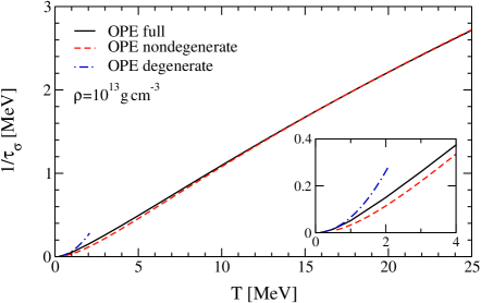
Figure 4: Spin relaxation rate $1/\tau_{\sigma}$ versus temperature $T$ based on the one-pion-exchange (OPE) approximation, comparing the full (partially degenerate) results to the nondegenerate and degenerate limits. The top and bottom panels are for density $\rho=10^{14}\,\text{g}\,\text{cm}^{-3}$ and $\rho=10^{13}\,\text{g}\,\text{cm}^{-3}$, respectively. The degenerate curves stop at $T=T_{\rm F}/\pi$. The inset shows the crossover region from the degenerate to the nondegenerate regime.

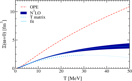
Figure 5: $\Xi(\omega=0)$ [Equation (40)] versus temperature $T$ based on the OPE approximation and from chiral NN interactions at N³LO, with a fitting curve to the central value of the band. The N³LO band is due to different NN potentials employed (Entem & Machleidt, 2003; Epelbaum et al., 2005). In addition, we show results based on the T matrix for NN scattering using phase shifts and mixing angles from NN-OnLine (2011) for $E_{\rm lab}\leqslant 350\,\text{MeV}$. For temperatures $T\gtrsim 30\,\text{MeV}$, the T matrix results are shown by a thin line, because contributions from higher $E_{\rm lab}$ to $\Xi(\omega=0)$ can become important.

We now consider how good the expression for the spin relaxation rate in the nondegenerate limit is under relevant conditions encountered in simulations of core-collapse supernovae. As representative of conditions during outflow, based on Figures 1 and 2, we take for values of the density ranging between $\rho_{0}/100$ and $\rho_{0}$ the temperature given by Equation (2).

In Figure 6, the full (partially degenerate) results are compared to the nondegenerate limit for these conditions. This figure demonstrates that results for the nondegenerate limit are an excellent approximation for matter in supernova simulations at subnuclear densities. Moreover, for the broad density range considered, the results based on N³LO NN potentials are similar to those based on the NN T matrix, and both lead to spin relaxation rates that are a factor two or more smaller compared to the OPE approximation.

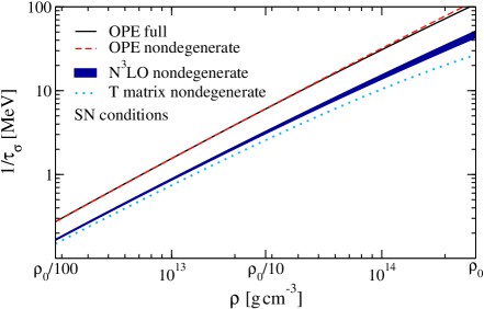
Figure 6: Spin relaxation rate $1/\tau_{\sigma}$ versus density $\rho$ for conditions typical of the outflow phase in supernova simulations [given by Equation (2)]. The full (partially degenerate) results are compared to the nondegenerate limit for the OPE approximation. In addition, we show the spin relaxation rate based on chiral NN interactions at N³LO and based on the T matrix for NN scattering. Note that the density dependence is linear in the nondegenerate limit [see Equation (41)].

Next, we study the dependence of the spin relaxation rate in the nondegenerate limit on frequency. When $\omega\neq 0$, the matrix elements that enter the rate are off-shell for $p\neq p^{\prime}=\sqrt{p^{2}+m^{*}\omega}$ [see Equation (50)], because the energies of the particles in the initial and final states differ by $\omega$. Figure 7 shows $\Xi(\omega)$ as a function of $\omega/T$ for the OPE interaction for three different temperatures, and compares the exact $\omega$ dependence with results in the on-shell approximation, where the partial-wave matrix elements are evaluated at a mean energy $V\bigl{(}\sqrt{p^{2}+m^{*}\omega/2},\sqrt{p^{2}+m^{*}\omega/2}\bigr{)}$. The differences are found to be small, because the momentum dependence of the interaction matrix elements varies on a scale of the order of the pion mass (and higher momenta for chiral EFT interactions), which is large compared to the energy transfer, which is of the order of the temperature. This conclusion is reinforced by the plots of the relative difference of the spin relaxation rate calculated with the exact $\omega$ dependence compared to the on-shell approximation in Figure 8 for typical conditions in supernova simulations.

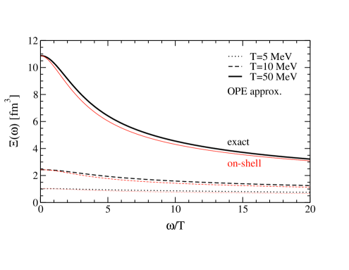
Figure 7: $\Xi(\omega)$ [Equation (40)] versus $\omega/T$ for temperatures $T=5,10,50\,\text{MeV}$. The results are based on the OPE approximation. Thick (thin) lines are for the exact $\omega$ dependence (on-shell approximation, see text).

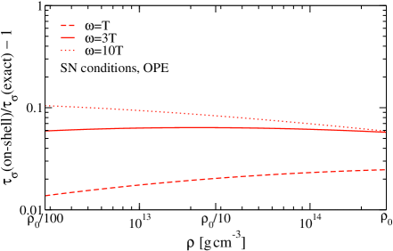
Figure 8: Relative difference, $\tau_{\sigma}(\text{on-shell})/\tau_{\sigma}(\text{exact})-1$, versus density $\rho$ based on the OPE approximation, comparing the exact $\omega$ dependence to the on-shell approximation (see text) for $\omega=T,3T$, and $10T$. The comparison is for conditions typical of the outflow phase in supernova simulations [given by Equation (2)].

For astrophysical applications, the quantity that enters the rates of neutrino processes is the spin dynamical structure factor which is related to the relaxation rate by Equations (4) and (14). In Figure 9, we plot the structure factor for two different densities, $10^{13}\,\text{g}\,\text{cm}^{-3}$ and $10^{14}\,\text{g}\,\text{cm}^{-3}$ [with corresponding temperatures given by Equation (2)]. The blue bands show the results for the N³LO NN potentials and the solid lines those for the OPE approximation calculated within the formalism of this paper. As one would expect from the fact that the width of the peak in the structure factor is proportional to the relaxation rate and its height is inversely proportional to the rate, the results for the N³LO interactions have a higher peak value and a narrower width compared with those for the OPE approximation. As representative of earlier work, we show as dotted lines results for the OPE calculations of Hannestad & Raffelt (1998) as implemented in the Basel code for core-collapse supernova simulations (Fischer et al., 2012). For a density of $10^{14}\,\text{g}\,\text{cm}^{-3}$, the Hannestad & Raffelt (1998) results lie 30-60% below our OPE results, while at $10^{13}\,\text{g}\,\text{cm}^{-3}$, the difference is generally less. The difference between the OPE results may be a consequence of imposing a normalization condition in Hannestad & Raffelt (1998), while in our approach the width is obtained consistently by solving the Boltzmann equation. For the comparison in Figure 9, we have neglected the frequency dependence of the relaxation rate, which is weak at these temperatures and would increas the structure factor with increasing $\omega/T$ (see Figure 7), as well as Fermi liquid corrections [$g_{0}=0$ in Equation (14)], which are not included in Hannestad & Raffelt (1998).

In scattering, the energy transfer to or from neutrinos is comparable to the width of the peak in the structure factor, and thus one sees that the energy transfer under realistic supernova conditions can be comparable to the temperature. It is important in future simulations to allow for this energy transfer. In addition, the rate of neutrino pair bremsstralung is roughly proportional to the spin relaxation rate, and therefore the N³LO results predict a lower rate for this process than does the OPE approximation. This is consistent with what has previously been found for degenerate conditions (Bacca et al., 2009). More comprehensive comparisons of predictions for rates of neutrino processes will be presented in future work that will extend the present calculations to take into account the effect of protons.

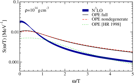
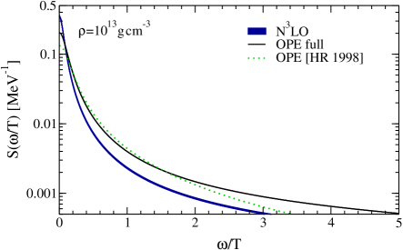
Figure 9: Spin dynamical structure factor $S(\omega/T)$ at long wavelength $q=0$ as a function of energy transfer $\omega$ divided by the temperature $T$ for densities $10^{14}\,\text{g}\,\text{cm}^{-3}$ (upper panel) and $10^{13}\,\text{g}\,\text{cm}^{-3}$ (lower panel). The corresponding temperatures are given by Equation (2). The blue bands show our results based on chiral NN interactions at N³LO, while the solid lines show results for the OPE approximation. For $\rho=10^{14}\,\text{g}\,\text{cm}^{-3}$, we also compare the nondegenerate approximation (dashed line) with the full OPE results, while at $10^{13}\,\text{g}\,\text{cm}^{-3}$ the results for the nondegenerate approximation are indistinguishable from the full calculation on the scale of the figure. The dotted lines show the OPE results of Hannestad & Raffelt (1998) [HR 1998] as implemented in the Basel code for core-collapse supernova simulations (Fischer et al., 2012).

6 Concluding remarks

We have analyzed simulations of core-collapse supernovae and have shown that in the post-bounce phase the relevant conditions for neutrino processes are partially degenerate or nondegenerate. We then developed a formalism for calculating neutrino rates in strongly interacting matter by generalizing to the partially degenerate regime the approach used for degenerate matter in Lykasov et al. (2008). The resulting spin dynamical structure factor takes into account both mean-field effects and collisions between excitations in neutron matter. We then calculated the spin relaxation rate, a key ingredient in the structure factor which enters expressions for the rates of neutrino processes. This was done at two levels of NN interactions, the OPE approximation, which is commonly used in simulations (Hannestad & Raffelt, 1998), and chiral EFT interactions. We have found that chiral NN interactions lead to a reduction of the spin relaxation rate typically by a factor of two for a broad range of conditions. This reduction is similar to what previously has been found in the degenerate regime (Bacca et al., 2009). We have also found that our OPE rate, where the width is obtained consistently by solving the Boltzmann equation, differs from the OPE results of Hannestad & Raffelt (1998). This may be a consequence of the imposition of a normalization condition in Hannestad & Raffelt (1998). Moreover, our results demonstrate that the nondegenerate limit is an excellent approximation for the conditions encountered in the post-bounce phase of matter at subnuclear densities in supernova simulations.

Future directions include the study of many-body contributions and of many-body forces and electroweak currents in chiral EFT, and the extension of the calculations to mixtures of neutrons and protons, where the central parts of nuclear interactions can cause relaxation of the axial charge, because of the different axial charges of the neutron and proton. These extensions will be greatly simplified by the finding that the nondegenerate limit provides an excellent approximation for the relevant supernova conditions.

Throughout the paper we have assumed that the basic coupling of the weak neutral field (that of the $Z$ boson) to nucleons is via a one-body operator. However, the spin relaxation effect that we have considered amounts to coupling a single quasiparticle-quasihole pair to two quasiparticle-quasihole pairs. In other words, strong interactions have generated a two-body contribution to the weak charge operator. However, not all two-body contributions to the operator are included in calculating relaxation effects by this procedure. The approximation we have made includes only contributions with a single quasiparticle in an intermediate state, which are enhanced by $1/\omega$. Consideration of other two-body contributions to the weak charge operator is left for future studies.

References

- Ardeljan et al. (2004) Ardeljan, N. V., Bisnovatyi-Kogan, G. S., Kosmachevskii, K. V., & Moiseenko, S. G. 2004, Astrophysics 47, 37
- Bacca et al. (2009) Bacca, S., Hally, K., Pethick, C. J., & Schwenk, A. 2009, Phys. Rev. C 80, 032802
- Baym & Pethick (1991) Baym, G. & Pethick, C. J. 1991, Landau Fermi Liquid Theory: Concepts and Applications (New York, Wiley)
- Bethe & Wilson (1985) Bethe, H. A. & Wilson, J. R. 1985, Astrophys. J. 295, 14
- Blondin et al. (2003) Blondin, J. M., Mezzacappa, A., & DeMarino, C. 2003, Astrophys. J. 584, 971
- Brandt et al. (2011) Brandt, T. D., Burrows, A., Ott, C. D., & Livne, E. 2011, Astrophys. J. 728, 8
- Brown & Jackson (1976) Brown, G. E. & Jackson, A. D. 1976, The Nucleon-Nucleon Interaction (North-Holland Amsterdam)
- Bruenn et al. (2001) Bruenn, S. W., De Nisco, K. R., & Mezzacappa, A. 2001, Astrophys. J. 560, 326
- Bruenn et al. (2009) Bruenn, S. W., Mezzacappa, A., Hix, W. R., Blondin, J. M., Marronetti, P., Messer, O. E. B., Dirk, C. J., & Yoshida, S. 2009, J. Phys.: Conf. Ser. 180, 012018
- Buras et al. (2006) Buras, R., Rampp, M., Janka, H.-T., & Kifonidis, K. 2006, Astronomy & Astrophysics 447, 1049
- Burrows & Sawyer (1998) Burrows, A. & Sawyer, R. F. 1998, Phys. Rev. C 58, 554
- Burrows et al. (2006) Burrows, A., Reddy, S., & Thompson, T. A. 2006, Nucl. Phys. A 777, 356
- Burrows et al. (2007) Burrows, A., Livne, E., Dessart, L., Ott, C. D., & Murphy, J. 2007, Astrophys. J. 655, 416
- Carneiro & Pethick (1975) Carneiro, G. M. & Pethick, C. J. 1975, Phys. Rev. B 11, 1106
- Chapman & Cowling (1970) Chapman, S. & Cowling, T. G. 1970, The Mathematical Theory of Nonuniform Gases, 3rd Edition (Cambridge University Press)
- Colgate & White (1966) Colgate, S. A. & White, R. H. 1966, Astrophys. J. 143, 626
- Cutkosky (1960) Cutkosky, R. E. 1960, J. Math. Phys. 1, 429
- Dasgupta et al. (2010) Dasgupta, B., Fischer, T., Horiuchi, S., et al. 2010, Phys. Rev. D 81, 103005
- Entem & Machleidt (2003) Entem, D. R. & Machleidt, R. 2003, Phys. Rev. C 68, 041001(R)
- Epelbaum et al. (2005) Epelbaum, E., Glöckle, W., & Meißner, U.-G. 2005 Nucl. Phys. A 747, 362
- Fischer et al. (2009) Fischer, T., Whitehouse, S. C., Mezzacappa, A., Thielemann, F., & Liebendörfer, M. 2009, Astronomy & Astrophysics 499, 1
- Fischer et al. (2012) Fischer, T., Martinez-Pinedo, G., Hempel, M., & Liebendörfer, M. 2012, Phys. Rev. D 85, 083003
- Foglizzo et al. (2007) Foglizzo, T., Galletti, P., Scheck, L., & Janka, H.-T. 2007, Astrophys. J. 654, 1006
- Freedman et al. (1977) Freedman, D. Z., Schramm, D. N., & Tubbs, D. L 1977, Annu. Rev. Nucl. Sci. 27, 167
- Hanhart et al. (2001) Hanhart, C., Philips, D. R., & Reddy, S. 2001, Phys. Lett. B 499, 9
- Hannestad & Raffelt (1998) Hannestad, S. & Raffelt, G. 1998, Astrophys. J. 507, 339
- Hebeler et al. (2010) Hebeler, K., Lattimer, J. M., Pethick, C. J., & Schwenk, A. 2010, Phys. Rev. Lett. 105, 161102
- Herant et al. (1994) Herant, M., Benz, W., Hix, W. R., Fryer, C. L., & Colgate, S. A. 1994, Astrophys. J. 435, 339
- Horowitz & Schwenk (2006) Horowitz, C. J. & Schwenk, A. 2006, Phys. Lett. B 642, 326
- Iwamoto & Pethick (1982) Iwamoto, N. & Pethick, C. J. 1982, Phys. Rev. D 25, 313
- Kotake et al. (2006) Kotake, K., Sato, K., & Takahashi, K. 2006, Rep. Prog. Phys. 69, 971
- Landau (1959) Landau, L. D. 1959, Nucl. Phys. 13, 181
- Langer (1961) Langer, J. S. 1961, Phys. Rev. 124, 997
- Langer (1962) Langer, J. S. 1962, Phys. Rev. 127, 5
- Lattimer & Swesty (1991) Lattimer, J. M. & Swesty, F. D. 1991, Nucl. Phys. A 535, 331
- Liebendörfer et al. (2001) Liebendörfer, M., Mezzacappa, A., Thielemann, F.-K., Messer, O. E. B., Hix, W. R., & Bruenn, S. W. 2001, Phys. Rev. D 63, 103004
- Liebendörfer et al. (2003) Liebendörfer, M., Mezzacappa. A., Messer, O. E. B., Martinez-Pinedo, G., Hix, W. R., & Thielemann, F.-K. 2003, Nucl. Phys. A 719, 144
- Liebendörfer et al. (2004) Liebendörfer, M., Messer, O. E. B., Mezzacappa, A., Bruenn, S. W., Cardall, C. Y., & Thielemann, F.-K. 2004, Astrophys. J. Suppl. 150, 263
- Lykasov et al. (2005) Lykasov, G. I., Olsson, E., & Pethick, C. J. 2005, Phys. Rev. C 72, 025805. In this paper, the expressions for in Section IV should all be multiplied by a factor of 2.
- Lykasov et al. (2008) Lykasov, G. I., Pethick, C. J., & Schwenk, A. 2008, Phys. Rev. C 78, 045803
- Marek & Janka (2009) Marek, A. & Janka, H.-T. 2009, Astrophys. J. 694, 664
- Menendez et al. (2011) Menendez, J., Gazit, D. & Schwenk, A. 2011, Phys. Rev. Lett. 107, 2011
- NN-OnLine (2011) NN-OnLine 2011, http://nn-online.org
- Olsson & Pethick (2002) Olsson, E. & Pethick, C. J. 2002, Phys. Rev. C 66, 065803
- Olsson et al. (2004) Olsson, E., Haensel, P., & Pethick, C. J. 2004, Phys. Rev. C 70, 025804
- Ott (2009) Ott, C. D. 2009, Classical & Quantum Gravity 26, 204015
- Pethick & Schwenk (2009) Pethick, C. J. & Schwenk, A. 2009, Phys. Rev. C 80, 055805
- Raffelt (1996) Raffelt, G. G. 1996, Stars as Laboratories for Fundamental Physics (University of Chicago Press), Section 4.3.1
- Raffelt & Seckel (1995) Raffelt, G. & Seckel, D. 1995, Phys. Rev. D 52, 1780
- Raffelt et al. (1996) Raffelt, G., Seckel, D. & Sigl, G. 1996, Phys. Rev. D 54, 2784
- Rampp et al. (2002) Rampp, M. & Janka, H.-T. 2002, Astronomy & Astrophysics 396, 361
- Reddy et al. (1998) Reddy, S., Prakash, M., & Lattimer, J. M. 1998, Phys. Rev. D 58, 013009
- Reddy et al. (1999) Reddy, S., Prakash, M., Lattimer, J. M., & Pons, J. A. 1999, Phys. Rev. C 59, 2888
- Sagert et al. (2009) Sagert, I., Fischer, T., Hempel, M., et al. 2009, Phys. Rev. Lett. 102, 081101
- Sawyer (1975) Sawyer, R. F. 1975, Phys. Rev. D 11, 2740
- Schwenk et al. (2003) Schwenk, A., Friman, B., & Brown, G. E. 2003, Nucl. Phys. A 713, 191
- Shen et al. (1998) Shen, H., Toki, H., Oyamatsu, K., & Sumiyoshi, K. 1998, Prog. Theor. Phys. 100, 1013
- Steiner et al. (2010) Steiner, A. W., Lattimer, J. M., & Brown, E. F. 2010, Astrophys. J. 722, 33
- Sumiyoshi et al. (2007) Sumiyoshi, K., Yamada, S., & Suzuki, H. 2007, Astrophys. J. 667, 382
- Suwa et al. (2010) Suwa, Y., Kotake, K., Takiwaki, T., Whitehouse, S. C., Liebendörfer, M., & Sato, K. 2010, Publ. Astron. Soc. Jap. 62, L49
- Taylor (1960) Taylor, J. C. 1960, Phys. Rev. 117, 261
- Thompson et al. (2003) Thompson, T. A., Burrows, A., & Pinto, P. A. 2003 Astrophys. J. 592, 434