Structural Susceptibility and Separation of Time Scales in the van der Pol Oscillator

Abstract

We use an extension of the van der Pol oscillator as an example of a system with multiple time scales to study the susceptibility of its trajectory to polynomial perturbations in the dynamics. A striking feature of many nonlinear, multi-parameter models is an apparently inherent insensitivity to large magnitude variations in certain linear combinations of parameters. This phenomenon of “sloppiness” is quantified by calculating the eigenvalues of the Hessian matrix of the least-squares cost function. These typically span many orders of magnitude. The van der Pol system is no exception: Perturbations in its dynamics show that most directions in parameter space weakly affect the limit cycle, whereas only a few directions are stiff. With this study we show that separating the time scales in the van der Pol system leads to a further separation of eigenvalues. Parameter combinations which perturb the slow manifold are stiffer and those which solely affect the jumps in the dynamics are sloppier.

I Introduction

In this manuscript, we analyze the sensitivity of a multiple time scales dynamical system to perturbative changes in its evolution laws. Rather than utilizing the traditional means of examining the structural stability for probing qualitative changes to the attractor as a response to perturbations, we study the structural susceptibility for quantifying the effects of the perturbations on the time series . More specifically, we ask how sensitive is the dynamical system $d\textbf{z}/dt=\textbf{f}(\textbf{z})$ to infinitesimal changes of the form $d\textbf{z}/dt=\textbf{f}(\textbf{z})+\textbf{a}\cdot\textbf{g}(\textbf{z})$, for a family of perturbations $\textbf{g}(\textbf{z})$ when the parameters $\textbf{a}\rightarrow\textbf{0}$.

This report introduces the new concept of “structural susceptibility” in dynamical systems, and is an outgrowth of our group’s previous work on “sloppiness” in multiparameter systems wherein we have found that data-fitting in a number of nonlinear, multiparameter models is only sensitive to a few directions in parameter space at the best fit BrownSethna ; Guntenkunst1 ; MarkLongPaper . The key difference between studying sloppiness and structural susceptibilities is that in the former, the parameters are intrinsic to the system, i.e., there are no externally introduced changes in their evolution laws. Nonetheless, the methodology we have developed for studying sloppy models is also suited for studying structural susceptibilities of dynamical systems. Our approach cleanly isolates and ranks the directions in parameter space in order of relevance to observed behavior, and has previously led us to suggest improvements in experimental design Optimal , extract falsifiable predictions from experiments Falsify , and develop faster minimization algorithms MarkLM . Others have developed our ideas to suggest further improvements in experimental design Apgar and parameter estimation Secrier , to quantify robustness to parameter variations Dayarian , and to set confidence regions for predictions in multiscale models Multiscale . In this paper, we bring similar ideas together to analyze sensitivities of time series to perturbations in dynamical systems.

We demonstrate the utility of our approach with application to a dynamical system with two time scales— the van der Pol oscillator VDP which is a single parameter system and hence not amenable to sloppy model analysis. Instead, by choosing appropriate perturbations $\textbf{g}(\textbf{z})$, we calculate the susceptibility of its dynamics: We make perturbations on the attractor, and then systematically increase the separation of time scales in its dynamics to show how it can generally enhance the sloppiness in nonlinear systems.

II Multiple Time Scale Dynamics

Multiple time scales are often found in the solutions of dynamical systems Jones . Broadly speaking, the defining criterion of these models is that the trajectory of one or more phase variables has an identifiable fast piece such as a jump or a pulse and a slow piece where the value of the variable doesn’t change quickly GrasmanBook . In two dimensions, these systems are commonly studied in the contexts of slow-fast vector fields written as:

$$\begin{array}[]{rl}\epsilon\dot{x}&=X(x,y,\epsilon),\\ \dot{y}&=Y(x,y,\epsilon)\end{array}$$ (1)

where the parameter $\epsilon>0$ is small and dot indicates derivative with respect to time $t$. For ${\cal O}(1)$ functions $X$ and $Y$, and $X\neq 0$: $\dot{x}={\cal O}(1/\epsilon)$ and $\dot{y}={\cal O}(1)$, so that $\epsilon$ is the ratio of time scales in the system. On one extreme, the singular limit $\epsilon=0$ corresponds to a differential algebraic system $X=0,\ Y=\dot{y}$ where the solutions of $X=0$ comprise the “critical manifold” close to which the flow in phase space is slow (the “slow manifold”). Similarly, $\epsilon=1$ corresponds to a limit where there is no separation of time scales, with a crossover at intermediate values of $\epsilon$.

Originally introduced in 1927, the van der Pol equation, $\ddot{x}-\mu(1-x^{2})\dot{x}+x=0$, is a well-studied example of a second-order, nonlinear system with multiple time scales in its solution. Using the Liénard transformation $y=x-x^{3}/3-\dot{x}/\mu$, and redefining time $t\rightarrow t\mu$, the equation can be written as a two dimensional system GrasmanBook ; Strogatz given by:

$$\begin{array}[]{rl}\mu^{-2}\dot{x}&=x-\frac{x^{3}}{3}-y,\\ \dot{y}&=x,\end{array}$$ (2)

which has the same form as (1) with $\epsilon=\mu^{-2}$. The global attractor of this dynamical system is a structurally stable limit cycle with two time scales .

The van der Pol system provides a convenient way to separate time scales by varying $\mu$: Small values of $\mu$ in the van der Pol system correspond to a small separation of time scales. It can be shown that the trajectory approaches that of the harmonic oscillator as $\mu\rightarrow 0$ VDP . At large values of $\mu$, the system shows a separation of time scales which increases with increasing $\mu$. As shown in figure 1 (b, c), with increasing $\mu$, the trajectory of $x$ separates into a slow part that lies ${\cal O}(exp(\mu^{-2}))$ close to the phase space curve given by $\dot{x}=0$, i.e. the critical manifold $y=x-x^{3}/3$, and a fast part which connects the two branches of the slow flow. Likewise, the separation of time scales in $y$ are associated with the increasing sharpness of the kink in its trajectory.

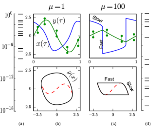
Figure 1: (a) Eigenvalues of the Hessian matrix of the cost of fitting at $\mu=1$, and (b, c top row) one period of time series x($\tau$) and y($\tau$), for $0<\tau<1$, are shown for $\mu=1$ and $\mu=100$ as function of time along with schematic error bars for the data-fitting of the trajectory of variable $y$. (d) Eigenvalues for $\mu=100$ are shown on the right. As $\mu\rightarrow\infty$, the orbit collapses onto the critical manifold with the trajectory spending most of its time on the slow manifold and vanishingly short on the jumps. Also shown in (b, c bottom row) is the orbit in $xy$ plane (solid line) and the critical manifold (dashed line).

The fact that with an increasing separation of time scales the trajectory spends an increasing amount time on the slow manifold and a decreasing amount of time on the jumps has important implications for fitting parameters to time series data of the van der Pol system. With increasing scale separation, one expects that the cost of fitting will be decreasingly sensitive to changes in the jumps of the trajectory as they get progressively shorter in duration.

III Sloppiness in Nonlinear Fits

In this section, we discuss the concepts of sloppiness and structural susceptibility in more detail with examples as a prelude to our calculations. For time series $z(t,\textbf{a})$, a least-squares fit to data $d_{i}$ minimizes a cost $C=\frac{1}{2}\sum_{i}(z(t_{i},\textbf{a})-d_{i})^{2}/\sigma_{i}^{2}$ in the space of system parameters which are collectively denoted as a. Our discovery of sloppiness is essentially that the eigenvalues of the Hessian of the cost with respect to parameters, ${\cal H}_{\alpha\beta}=\partial^{2}C/\partial a_{\alpha}\partial a_{\beta}$, at the best fit span many orders of magnitude. The larger and smaller eigenvalues correspond to stiffer and sloppier directions respectively. For concreteness, consider a time series of a multi parameter model, such as the one denoted by $y(\tau)$ in figure 1(b, top row). The error bars schematically show the least-squares fit of $y(\tau)$ and the sidebar (figure 1(a)) shows the eigenvalues of the corresponding Hessian matrix. Note the broad range of eigenvalues ($\sim 10^{11}$, corresponding to a factor of almost a million in parameter range)— a feature that turns out to be typical in nonlinear fits.

Another vivid example of sloppiness in nonlinear models is provided by the well-established formalism behind the characterization of the sensitivities of initial conditions using Lyapunov exponents Katok . Consider $d\textbf{z}/dt=\textbf{f}(\textbf{z})$ as a model whose parameters are the initial conditions $a_{\alpha}=z_{\alpha}(0)$ and whose predictions are the final positions $z_{i}(t)$ at time $t$. At the best fit, ${\cal H}_{\alpha\beta}=(J^{T}J)_{\alpha\beta}$ where $J_{i\alpha}=\partial z_{i}(t)/\partial z_{\alpha}(0)$ is the Jacobian of the sensitivities to perturbations in the initial conditions. The Lyapunov exponents, which are defined to be the eigenvalues $\ell_{n}$ of $\textbf{L}=\lim_{t\to\infty}1/(2t)\log(J^{T}J)$, utilize the same Hessian we would use in calculating the sloppy model eigenvalues $\lambda_{n}=exp(2t\ell_{n})$. The roughly equal spacing of Lyapunov exponents naturally explains both the exponentially broad range of sloppy model exponents and the roughly equal spacing of $\log(\lambda_{n})$ for a model with initial conditions as parameters.

Instead of the sensitivities with respect to the initial conditions or other intrinsic parameters, we focus here on the sensitivity of the dynamics to changes in the dynamical evolution laws. Therefore, for the remainder of this paper we will be interested in a cost function that measures the square of the distance between two time series for the system $d\textbf{z}/dt=\textbf{f(z)}+\textbf{a}\cdot\textbf{g}(z)$— one with perturbations— $\textbf{z}(t,\textbf{a}\rightarrow\textbf{0})$, and the other one without, i.e., $\textbf{z}(t,\textbf{a=0})$

$$C=\frac{1}{2}\int_{0}^{T}\!||\textbf{z}(t,\textbf{a}\rightarrow\textbf{0})-\textbf{z}(t,\textbf{a}=\textbf{0})||^{2}\,\mathrm{d}t$$ (3)

with the perturbing terms $g_{i}(z)$ giving a power series in the components of z. Further in the manuscript, we will use this form of the cost to compute the susceptibility of the van der Pol system and show how sloppiness is enhanced by increasing separation of time scales in the van der Pol equations. This is in essence captured by figure 1(a & d) where we show that an increase in the van der Pol parameter $\mu$ from $1$ to $100$ produces roughly a million-fold increase in the spread of eigenvalues.

IV Susceptibility of van der Pol system

We perturb the van der Pol system in (2) by adding a series of additional terms. There is a long tradition in dynamical systems of studying equations of motion of polynomial form Katok ; Gucken ; indeed, the theory of normal forms suggests that general dynamical systems, even at bifurcations, can be generically mapped into a polynomial form by a nonlinear but smooth change of variables. Adding extra polynomial terms is routinely done to ‘unfold’ the qualitative behavior near bifurcations Unfold . Here we focus on quantitative changes far from bifurcations. In choosing our perturbations, we must cut off the polynomials at some order. There are two ways in which we specialize our general susceptibility analysis to the two time scale, periodic limit cycle of the van der Pol system. First, we choose the family of perturbations of order $3N$ as follows:

$$\begin{array}[]{rl}\mu^{-2}\dot{x}&=x-\frac{x^{3}}{3}-y+\sum_{m+n\leq N}a_{m,n}(x-\frac{x^{3}}{3}-y)^{m}x^{n}\\ \dot{y}&=x.\end{array}$$

This choice has two noteworthy features— (a) We have grouped the polynomial perturbations so that, for $m\neq 0$ they vanish on the critical manifold, $y=x-x^{3}/3$. That is, the parameters $a_{m,n}$ with $m\neq 0$ do not significantly affect the dynamics on the slow manifold; we call these the “fast parameters” and correspondingly the $a_{0,n}$ are “slow parameters”. The parameter $a_{1,0}$ duplicates $\mu$ to the same effect as changing the period, and we omit it. Surely, the eigenvalue spectrum of the general polynomial expansion, $a_{m,n}x^{m}y^{n}$, behaves qualitatively similarly to the one presented here but our parametrization greatly simplifies the analysis of the eigenvector perturbations. (b) We only perturb the $\dot{x}$ equation. Our choice corresponds to a general expansion of a second-order equation, with the acceleration $\ddot{y}=\dot{x}$ written as a polynomial in the position $y$ and velocity $\dot{y}=x$. Perturbing both equations produces similar behavior.

Second, we modified the cost to focus on the limit cycle of the van der Pol system in two ways— (a) by rescaling all trajectories in our analysis so that they have the same unit period, and (b) by changing the initial condition so that it lies on the perturbed orbit and that the perturbed and unperturbed orbits are in phase with each other . When we correct the period $T$ by $\delta T$, initial conditions $\textbf{y}_{0}$ by $\delta\textbf{y}_{0}$, and do an overall rescaling of the time variable $t\rightarrow\tau T$, the cost functional for the time series of $y(\tau)$ at each $\mu$ takes the following form:

$$C(\mu)=\frac{1}{2}\int_{0}^{1}\![y(\tau,\textbf{a}+\delta\textbf{a},\textbf{y}_{0}+\delta\textbf{y}_{0},T+\delta T)-$$

$$y(\tau,\textbf{a},\textbf{y}_{0},T)]^{2}\,\mathrm{d}\tau$$ (4)

In principle, changes in both time series, $x(\tau)$ and $y(\tau)$ could be incorporated in the cost function, but we get qualitatively similar results by keeping either or both variables. Choosing to measure changes only in $y(\tau)$ corresponds again to studying the second-order equation for $\ddot{y}$ as an expansion in $y$ and $\dot{y}$.

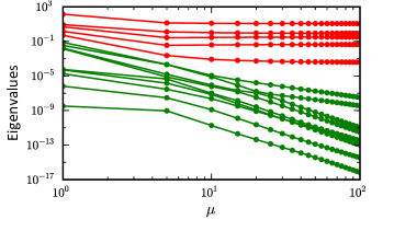
Figure 2: Eigenvalues of Hessian matrix are shown here as a function of $\mu$. The range $1\leq\mu\leq 100$ corresponds to a ratio of time scales $1\leq\epsilon\leq 10000$. The five largest eigenvalues correspond to stiff directions in the parameter space: these directions perturb the slow manifold. The remainder affect the transient part of the trajectory which becomes smaller with an increasing separation of time scales and hence these directions are decreasingly relevant.

The susceptibilities are still given by the Hessian matrix at the best fit (a=0):

$${\cal H}(\mu)_{\alpha\beta}=\frac{\partial^{2}C(\mu)}{\partial a_{\alpha}\partial a_{\beta}}$$ (5)

which can be written out more completely as:

$${\cal H}(\mu)_{\alpha\beta}=\int_{0}^{1}\!\left(\frac{\partial y}{\partial a_{\alpha}}+\frac{\partial y}{\partial\textbf{y}_{0}}\frac{\partial\textbf{y}_{0}}{\partial a_{\alpha}}+\frac{\partial y}{\partial T}\frac{\partial T}{\partial a_{\alpha}}\right)$$

$$\times\left(\frac{\partial y}{\partial a_{\beta}}+\frac{\partial y}{\partial\textbf{y}_{0}}\frac{\partial\textbf{y}_{0}}{\partial a_{\beta}}+\frac{\partial y}{\partial T}\frac{\partial T}{\partial a_{\beta}}\right)\,\mathrm{d}\tau$$

Here, each of the two terms in the integral is to be interpreted as a Jacobian matrix, a mapping from the finite dimensional parameter space to the infinite dimensional data space:

$$J_{\tau\alpha}=\frac{\partial y(\tau)}{\partial a_{\alpha}}+\frac{\partial y(\tau)}{\partial\textbf{y}_{0}}\frac{\partial\textbf{y}_{0}}{\partial a_{\alpha}}+\frac{\partial y(\tau)}{\partial T}\frac{\partial T}{\partial a_{\alpha}}$$ (6)

The sensitivity trajectories in the Jacobian, $\partial y/\partial a_{\alpha}$, $\partial y/\partial\textbf{y}_{0}$, and $\partial y/\partial T$, were computed using the open source SloppyCell package SloppyCell1 ; SloppyCell2 . The expressions for the time invariant quantities, $\partial\textbf{y}_{0}/\partial a_{\alpha}$ and $\partial T/\partial a_{\alpha}$, were found by enforcing periodicity of the perturbed time series denoted by $\textbf{y}(\tau)\equiv(x(\tau),y(\tau))$ as follows:

$$\textbf{y}(\tau=0,\textbf{a}+\delta\textbf{a},\textbf{y}_{0}+\delta\textbf{y}_{0},T+\delta T)=$$

$$\textbf{y}(\tau=1,\textbf{a}+\delta\textbf{a},\textbf{y}_{0}+\delta\textbf{y}_{0},T+\delta T),$$

Taylor expansion of both sides of the previous equation leads to a vector equation:

$$\delta\textbf{y}_{0}=\frac{\partial\textbf{y}}{\partial T}\bigg{|}_{\tau=1}\delta T+\frac{\partial\textbf{y}}{\partial\textbf{a}}\bigg{|}_{\tau=1}\delta\textbf{a}+\frac{\partial\textbf{y}}{\partial\textbf{y}_{0}}\bigg{|}_{\tau=1}\delta\textbf{y}_{0},$$

from which both constants can be computed following the convention that the component denoting the change in initial condition of $y(\tau)$ in $\delta\textbf{y}_{0}$ is set to zero. Now with the Jacobian calculated, the Hessian at best fit is simply ${\cal H}=J^{T}J$.

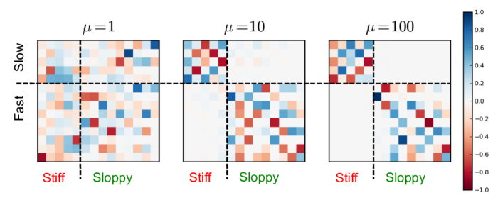
Figure 3: Hessian eigenvectors are shown for $\mu=1,\ 10,$ and $100$. Each colored small square shows the magnitude of an eigenvector component (the scale bar shown on the right). Eigenvectors for each $\mu$ are sorted so that the stiffer ones appear on the left; individual components are sorted so that “slow parameters” appear on the top. Note that with increasing $\mu$, the stiff and sloppy eigenvectors separate by parameters: The stiff eigenvectors only have projections along the slow parameters which perturb the slow manifold, whereas the sloppy directions have projections along the fast parameters which mainly perturb the jumps.

IV.1 Eigenvalues and Eigenvectors

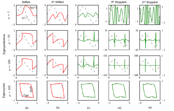
Figure 4: Top three rows: Eigenpredictions $\delta y_{k}$ for $k=0,\ 3,\ 6,\ 9,\ 12$ at $\mu=1,\ 10\ \&\ 100$ are shown in solid red lines for stiff modes and solid green for sloppy modes. These curves show the response of perturbations if the parameters are changed infinitesimally along the Hessian eigenvectors: A parameter change of norm $\epsilon$ along eigendirection $n$ will change the trajectories by $\lambda_{n}\epsilon$ times the eigenpredicton. Dashed lines show unperturbed van der Pol solution for comparison ($y$ scale on the right hand side). As the time scales separate, the amplitudes of the sloppiest eigenpredictions increase (roughly in proportion to $\mu$) getting increasingly concentrated at the jumps. Bottom row shows the eigencycles for $\mu=100$ in solid red lines corresponding to the perturbations in row 3 (i.e. the new limit cycle for a perturbation of strength $\epsilon\sim 1/\lambda_{n}$. These curves show how the van der Pol orbit changes with perturbations along the Hessian eigenvectors. Both the stiff and the sloppy modes change the orbit at the jumps (occurring at the extrema in the dashed lines); the stiff modes also change behavior at the slow manifold, whereas the sloppy modes only affect the jumps.

We computed the Hessian matrix given by the previous equation at multiple values of $\mu$. The spread of eigenvalues (figure 2) increases as a function of $\mu$ confirming that sloppiness increases with an increasing separation of time scales. Not surprisingly , for $N=4$, the $14$ eigenvalues for $\mu=1$ already span $11$ orders of magnitude, while for $\mu=100$, we observe that the stiffest eigenvalue is $18$ orders of magnitude larger than the smallest one— the spread increases by $10^{7}$ when $\mu$ increases to $100$.

Taken together with the eigenvectors shown in figure 3, some interesting facts come to light: Figure 2 shows that with increasing $\mu$, the eigenvalues separate into two clusters of closely related decay exponents. The largest $N$ eigenvalues approach constants. The other eigenvalues decay with power laws: two modes with exponents between $-2$ and $-3$ and the remaining with exponents between $-5$ and $-6$. Similarly, figure 3 shows that the eigenvectors also separate into two groups with increasing $\mu$: The stiffest directions are linear combinations of the slow parameters whereas the sloppy directions are comprised of other parameters as expected.

We can understand the effect of perturbations in parameter combinations given by the eigenvectors (called eigenparameters) $\hat{\textbf{e}}_{k}$ more clearly by observing their behavior in the data space. The Jacobian transformation of (6) projects the eigenvectors to the data space: $\delta y_{k}=J\cdot\hat{\textbf{e}}_{k}/\sqrt{\lambda_{k}}$ where ${\lambda_{k}}$ corresponds to the $k^{th}$ largest eigenvalue. Defined this way, these data space vectors, called eigenpredictions MarkLongPaper , $\delta y_{k}$, are also orthonormal. Alternatively, the eigenpredictions are the left singular vectors in the singular value decomposition of the Jacobian (i.e. they are the columns of the unitary matrix $U$ in $J=U\Sigma V^{T}$ NR ) As shown in figure 4 for $\mu=1,\ 10\ \&\ 100$ (top three rows), we learn from the eigenpredictions that the stiff modes affect behavior both along the slow manifold and at the jumps. Moreover with increasing $\mu$, as the eigenvalues associated with the stiff directions approach constants (figure 2), so do the stiff eigenpredictions (figure 4 rows 2, 3 columns (a) and (b)). The sloppy modes on the other hand, affect the dynamics on the jumps only. The maximum amplitudes of the (normalized) sloppiest eigenpredictions appears to increase roughly proportional to $\mu$ (corresponding to the jump duration of $\sim\mu^{-2}$). In the limit, these become $\delta$-functions and derivatives concentrated at the jumps. Figure 4 (bottom row) also shows the limit cycles (eigencycles) with eigenparameter perturbations as phase space trajectories $(x,y+\eta\ \delta y_{k})$ for small $\eta$.

V Discussion

In this paper, we have introduced a formalism we call “structural susceptibility” for analyzing the quantitative dependence of dynamical systems to perturbations of the equations of motion. It is a generalization of ‘unfolding’ methods of bifurcation theory and the Lyapunov exponents governing the dependence on initial conditions, and exposes the ubiquitous presence of broad range of sloppy eigendirections in parameter space— largely unimportant to the dynamics. We used this method to study the role of time scale separation in enhancing the sloppiness of the susceptibility spectrum in the particular case of the van der Pol oscillator.

By extending the framework of our sloppy model analysis to systems where changes in evolution laws are to be studied, our method offers a simple way to calculate the effects of broad classes of perturbations. By studying the structural susceptibility of a dynamical system with two time scales, the analysis presented here showed that sloppiness of nonlinear systems is enhanced by separation of time scales in the dynamics. With increasing separation of time scales in the van der Pol oscillator, the trajectory spends an increasing amount of time on the slow manifold and a vanishingly small amount of time in the transition region. The cost of perturbations is integrated over time and therefore we are unsurprised that the perturbations that change the slow manifold will accrue the most cost and therefore manifest as stiff modes of the Hessian matrix. The remaining directions are sloppy as they only affect the behavior at the jumps or the fast pieces. These perturbations manifest as $\delta$-functions and their derivatives— significantly affecting the phase-space trajectory, but over only the fast times asymptotically ignored in the least-squares cost. It remains a challenge to connect separation of time scales to parameter sensitivity in more complicated systems, but the analogy of the van der Pol system’s behavior with other nonlinear physical systems of interest is clear.

Many important dynamical systems have multiple time scales in their solutions: examples include models in neuroscience (such as Hodgkin-Huxley model), systems biology or chemical reaction systems (such as protein network models), and in engineering (such as models of combustion, lasers, locomotion, etc.). Our analysis suggests that any system with multiple time scales should become sloppier as the scales separate for the same reasons as we found in the van der Pol: Some parameter combinations will only affect the fast dynamics, and lead to sloppy modes. Perturbations which affect the slow dynamics will presumably accrue more cost and be stiff.

More broadly, the sloppiness exposed by our structural susceptibility analysis has clear implications for attempting to reconstruct the equations of motion from experimental data Lipson because the true dynamics along any sloppy eigendirection will be relatively poorly determined. This discovery has already influenced work on experimental design optimization: estimating parameters is challenging Apgar ; Comment , but extracting predictions without constraining parameters is straightforward Falsify . We further anticipate that the concept of structural susceptibility will be useful for studying systems with chaos, bifurcations and phase transitions; quantifying the unfoldings of these systems may also be useful for gaining a deeper understanding of the phenomena they model.

VI Acknowledgments

We thank Stefanos Papanikolaou for helpful conversations leading us to think about perturbing the slow manifold and about the analogues to thermodynamic susceptibilities, and John Guckenheimer for valuable insights and discussions regarding our calculations. Support from NSF grant DMR 1005479 is gratefully acknowledged.

References

- [1] We employ the word structural in the same context as its usage in dynamical systems literature on structural stability. The word susceptibility is inspired from physics wherein it is a measure of response to a perturbation (such as an applied external field) quantified by the second-derivative of the free energy w.r.t. parameters. Since cost is analogous to free energy (in that both are minimized), it is natural to call the response to perturbations in dynamics, also quantified via second derivatives, as structural susceptibility.
- [2] Kevin S. Brown and James P. Sethna. Statistical mechanical approaches to models with many poorly known parameters. Phys. Rev. E, 68:021904, Aug 2003.
- [3] Ryan N Gutenkunst, Joshua J Waterfall, Fergal P Casey, Kevin S Brown, Christopher R Myers, and James P Sethna. Universally sloppy parameter sensitivities in systems biology models. PLoS Comput Biol, 3(10):e189, 10 2007.
- [4] Mark K. Transtrum, Benjamin B. Machta, and James P. Sethna. Geometry of nonlinear least squares with applications to sloppy models and optimization. Phys. Rev. E, 83:036701, Mar 2011.
- [5] Fergel P. Casey, D. Baird, Q. Feng, R.N. Gutenkunst, J.J. Waterfall, C.R. Myers, K.S. Brown, R.A. Cerione, and J.P. Sethna. Optimal experimental design in an epidermal growth factor receptor signalling and down-regulation model. IET Systems Biology, 1(3):190–202, 2007.
- [6] Ryan N. Gutenkunst, Fergal P. Casey, Joshua J. Waterfall, Christopher R. Myers, and James P. Sethna. Extracting falsifiable predictions from sloppy models. Annals of the New York Academy of Sciences, 1115(1):203–211, 2007.
- [7] Mark K. Transtrum and James P. Sethna. Improvements to the levenberg-marquardt algorithm for nonlinear least-squares minimization.
- [8] Joshua F. Apgar, David K. Witmer, Forest M. White, and Bruce Tidor. Sloppy models, parameter uncertainty, and the role of experimental design. Mol. BioSyst., 6:1890–1900, 2010.
- [9] Maria Secrier, Tina Toni, and Michael P. H. Stumpf. The ABC of reverse engineering biological signalling systems. Mol. BioSyst., 5:1925–1935, 2009.
- [10] Adel Dayarian, Madalena Chaves, Eduardo D. Sontag, and Anirvan M. Sengupta. Shape, size, and robustness: Feasible regions in the parameter space of biochemical networks. PLoS Comput Biol, 5(1):e1000256, 01 2009.
- [11] Hannes Hettling and Johannes HGM van Beek. Analyzing the functional properties of the creatine kinase system with multiscale ‘sloppy’ modeling. PLoS Comput Biol, 7(8):e1002130, 08 2011.
- [12] Balthasar van der Pol. On relaxation-oscillations. The London, Edinburgh and Dublin Phil. Mag. & J. of Sci., 2(7):978–992, 1927.
- [13] Christopher K.R.T. Jones and Alexander I. Khibnik (Eds.). Multiple-time-scale dynamical systems. Springer, 2000.
- [14] Johan Grasman. Asymptotic Methods for Relaxation Oscillations and Applications. Springer Press, 1987.
- [15] Steven H. Strogatz. Nonlinear Dynamics and Chaos: With Applications to Physics, Biology, Chemistry and Engineering. Westview Press, 2001.
- [16] Incidentally, the set of equations (2) can also be considered a special case of the FitzHugh-Nagumo model (See R. FitzHugh. Impulses and Physiological States in theoretical models of nerve propagation Biophys J., 1(6):445, 1961) introduced three decades later as simplification of the Hodgkin-Huxley equations of neuronal spikes in the squid giant axons, and is sometimes referred to as the Bonhoeffer-van der Pol model.
- [17] Anatole Katok and Boris Hasselblatt. Introduction to the Modern Theory of Dynamical Systems. Cambridge University Press, 1997.
- [18] John M. Guckenheimer and Phillip Holmes. Nonlinear Oscillations, Dynamical Systems and Bifurcations of Vector Fields. Springer Press, 1983.
- [19] J. Murdock. Normal Forms and Unfoldings for Local Dynamical Systems. Springer, New York, 2003.
- [20] Perturbations distort the dynamics so that the attractor and its period change. We addressed these issues by setting the periods to unity, and by moving the initial conditions to the new attractor to remove any transients. Alternatively, if we fit data over many periods without making the said changes, the parameter combinations determining the period and phase would become stiff modes in our dynamics.
- [21] Ryan N. Gutenkunst, Jordan C. Atlas, Fergal P. Casey, Robert S. Kuczenski, Joshua J. Waterfall, Christopher R. Myers, and James P. Sethna. Sloppycell http://sloppycell.sourceforge.net. 2007.
- [22] Christopher R. Myers, Ryan N. Gutenkunst, and James P. Sethna. Python unleashed on systems biology. Computing in Science Engineering, 9(3):34 –37, 2007.
- [23] We understand this as sloppiness as arising due to the generalized interpolation argument [4].
- [24] William H. Press, Saul A. Teukolsky, William T. Vetterling, and Brian P. Flannery. Numerical Recipes 3rd Edition: The Art of Scientific Computing. Cambridge University Press, New York, NY, USA, 3 edition, 2007.
- [25] Josh Bongard and Hod Lipson. Automated reverse engineering of nonlinear dynamical systems. Proceedings of the National Academy of Sciences, 104(24):9943–9948, 2007.
- [26] Ricky Chachra, Mark K. Transtrum, and James P. Sethna. Comment on “Sloppy models, parameter uncertainty, and the role of experimental design”. Mol. BioSyst., 7:2522–2522, 2011.