A faster method of computation of lattice quark number susceptibilities

Abstract

We compute the quark number susceptibilities in two flavor QCD for staggered fermions by adding the chemical potential as a Lagrange multiplier for the point-split number density term. Since lesser number of quark propagators are required at any order, this method leads to faster computations. We propose a subtraction procedure to remove the inherent undesired lattice terms and check that it works well by comparing our results with the existing ones where the elimination of these terms is analytically guaranteed. We also show that the ratios of susceptibilities are robust, opening a door for better estimates of location of the QCD critical point through the computation of the tenth and twelfth order baryon number susceptibilities without significant additional computational overload.

I Introduction

Quantum Chromo Dynamics (QCD), the theory of strong interactions, may have a critical point in the temperature (T)-baryon number density (or the baryonic chemical potential $\mu_{B}$) depending on the number of light flavors it has. The search for this critical point is one of the major experimental goals of many heavy ion collider experiments world wide. In particular, the STAR experiment at the Brookhaven National Laboratory has begun an extensive Beam Energy Scan(BES) program mohanty . It aims to scan the QCD phase diagram for baryon chemical potential between 20 to around 400 MeV, looking for the signatures of the presence of the critical point. FAIR at GSI, Darmstadt, Germany and NICA at Dubna, Russia are proposed to be operational in future with a key objective as the search for and the study of, a QCD critical point. It, therefore, appears natural to have a first principles theoretical exploration of the QCD critical point, with a possible prediction for its location which could serve as a useful reference for these large scale experiments. The physics near the critical point is essentially non-perturbative. Lattice gauge theory is the most successful non-perturbative tool which can be used for such an exercise. Fluctuations of conserved charges like the baryon number or strangeness are sensitive indicators of the existence of singularities in the phase diagram like the critical point koch ; srs . It is expected that the baryon number susceptibility would diverge at the critical point. On a finite lattice, however, this quantity will show a peak at the critical point which would get sharper as the lattice volume is increased. The direct computation of the susceptibility at finite baryon density is difficult due to the infamous “fermion sign problem”. One of the techniques to circumvent the sign problem at finite density is to compute the baryon number susceptibility as a Taylor series expansion in chemical potential near zero alt1 ; alt2 ; gg3 . The radius of convergence of the series should yield an estimate of the location of the critical point gg1 . For the precise estimation of the radius of convergence, one needs to compute ratios of as many higher orders of baryon number susceptibilities as possible. Current state of the art is the eighth order susceptibility on the lattice gg2 . Higher order terms are important in determining the critical point, and extending to higher orders in Taylor series is therefore desirable although the explosion in the CPU time required is severely constraining.

There are two major issues that have to be addressed for the efficient computations of higher order quark number susceptibilities(QNS). Firstly, using the standard method of introducing chemical potential on the lattice hk ; kogut ; bilicgavai ; gavai , the computation of QNS beyond eighth order with reasonably good precision becomes rather expensive. At each order, the fermion matrix inversions account for the maximum time involved in computing the QNS. As shown in gg1 , twenty inversions are necessary for computing the eighth order susceptibility; it would increase to about forty for the tenth order. For computing higher orders of QNS on the lattice, the number of matrix inversions would thus increase drastically thereby increasing the computation time. Secondly the current estimates of the susceptibilities beyond fourth order on the lattice tend to become statistically demanding as they are rather noisy. This is due to the fact that there are delicate cancellations in the expressions of QNS between different terms. Moreover, the number of such terms itself increases progressively with the order of the susceptibility. Each term has to be computed with appropriate precision in order to ensure the cancellation of is free of computational artifacts. It would be desirable to reduce the number of such cancellations.

In this paper we attempt to address both these issues. We use a staggered fermion matrix in which the chemical potential, $\mu$, enters as a Lagrange multiplier, multiplying the point-split conserved number density term. It alleviates the problems mentioned above, as shown in  gs . For computing the eighth order QNS, only eight fermion matrix inversions would be needed gs as compared to the twenty required in the conventional method hk . In the early years of lattice computations this method of introducing $\mu$ linearly was discarded because the second order QNS computed using this term leads to a $1/a^{2}$ lattice term that diverges in the limit of vanishing lattice spacing, $a$. Modifications of the lattice action hk ; kogut ; bilicgavai ; gavai eliminated this term exactly for the free theory. In addition, they also ensured the correct Fermi surface on the lattice. These modifications lead to the difficulties in computing the higher order QNS though. It therefore appears a worthy attempt to focus back on the linear in $\mu$ action and devise ways to obtain physical answers. A method of successful elimination of the divergence maybe relevant in another context as well. The recently proposed overlap operator at finite density ns with exact chiral symmetry on the lattice has such a linear dependence in $\mu$. Indeed, the suggestions of  hk ; kogut ; bilicgavai ; gavai of divergence removal do not seem to work in that case.

Our paper is organized as follows. In Section II we briefly review the basic formulae of the various susceptibilities and show the differences in the two methods. In Section III we suggest a procedure to remove the lattice artifacts in the QNS computed with the linear term in $\mu$. Free fermion results are shown to yield the correct continuum limit with it. We then compare our results for full QCD with those in the standard exponential method hk . We show that our results are consistent with the existing results for different orders of QNS and the ratios of baryon number susceptibilities for a wide range of temperatures. A summary of our results along with possible sources of errors and their refinement is given in the last section.

II Formalism

The quark number susceptibilities(QNS) for two flavor QCD are defined as,

$$\chi_{ij}(\mu_{u},\mu_{d})=\frac{T}{V}\frac{\partial^{i+j}\ln Z(T,\mu_{u},\mu_{d},,m_{u},m_{d})}{\partial\mu_{i}\mu_{j}}$$ (1)

where $Z$ is the QCD partition function,

$$Z(T,\mu_{u},\mu_{d})=\int\mathcal{D}U\rm{e}^{-S_{G}}DetD_{u}^{\frac{1}{4}}DetD_{d}^{\frac{1}{4}}.$$ (2)

$S_{G}$ is the action for the gluon fields. We use the standard plaquette action for $S_{G}$. $D_{i}$, for each $i=u,d$, is the staggered fermion matrix in presence of finite quark chemical potentials. Several choices of the Dirac matrix are possible on the lattice at finite density. As in the continuum, the chemical potential can be introduced as a Lagrange multiplier corresponding to the conserved number density on the lattice in the point split form. This term is added to the standard staggered fermion matrix to yield the $D(\mu)$ which we use in this work:

$$D(\mu)_{xy} = D(0)_{xy}+\mu a\left[\eta_{4}U^{\dagger}_{4}(y)\delta_{x,y+\hat{4}}+\eta_{4}U_{4}(x)\delta_{x,y-\hat{4}}\right]$$ (3)

$$= \sum_{i=1}^{3}\left[\eta_{i}U_{i}(x)\delta_{x,y-\hat{i}}-\eta_{i}U^{\dagger}_{i}(y)\delta_{x,y+\hat{i}}\right]-(1-\mu a)\eta_{4}U^{\dagger}_{4}(y)\delta_{x,y+\hat{4}}+(1+\mu a)\eta_{4}U_{4}(x)\delta_{x,y-\hat{4}}+ma~{}\delta_{x,y}.$$

$\eta_{i}$ are the phase factors remnants of the gamma matrices as usual. Replacing $(1\pm\mu a)$ by exp$(\pm\mu a)$, one obtains the popular method hk of introducing $\mu$. We shall compare our results with those obtained by employing the latter.

In general, the chemical potentials $\mu_{i}$ and $\mu_{j}$, for quark flavors i and j respectively need not be the same. But since isospin is a good symmetry for QCD, we set the chemical potentials for up and down quarks to be the same, $\mu_{u}=\mu_{d}=\mu$. Hence the baryon chemical potential is just $\mu_{B}=3\mu$. The baryon number susceptibilities can then be expressed in terms of the quark number susceptibilities(QNS) $\chi_{ij}$. For two flavor QCD, the expressions for baryon number susceptibility of n-th order, $\chi_{B}^{n}$, are

$$\chi_{B}^{(4)} = \frac{1}{2}\left[\chi_{40}+2\chi_{31}+\chi_{22}\right]~{},~{}$$

$$\chi_{B}^{(6)} = \frac{1}{4!}\left[\chi_{60}+4\chi_{51}+7\chi_{42}+4\chi_{33}\right]~{},~{}$$

$$\chi_{B}^{(8)} = \frac{1}{6!}\left[\chi_{80}+6\chi_{71}+16\chi_{62}+26\chi_{53}+15\chi_{44}\right]~{}.$$ (4)

In this work we would be interested in computing the baryon number susceptibilities at $\mu_{B}=0$ since these quantities appear in the Taylor series expansion of the second order baryon number susceptibility expressed in powers of $\mu_{B}$,

$$\frac{\chi_{20}(\mu_{B})}{T^{2}}=\frac{\chi_{20}(0)}{T^{2}}+\chi^{(4)}_{B}\left(\frac{\mu_{B}}{3T}\right)^{2}+\chi^{(6)}_{B}\left(\frac{\mu_{B}}{3T}\right)^{4}+\chi^{(8)}_{B}\left(\frac{\mu_{B}}{3T}\right)^{6}+..$$ (5)

If a critical point exist then the baryon number susceptibility should diverge at that point in the continuum limit. The radius of convergence of this series, should therefore determine the location of the critical point in the $T$-$\mu_{B}$ plane of the QCD phase diagram. It can be defined as

$$r_{n}=\lim_{n\rightarrow\infty}\sqrt{\frac{\chi_{B}^{(n+1)}}{\chi_{B}^{(n+3)}}}~{},~{}{~{}~{}~{}\rm or~{}~{}~{}}r_{n}=\lim_{n\rightarrow\infty}\left[\frac{\chi_{B}^{(2)}}{\chi_{B}^{(n+2)}}\right]^{1/n}~{}.$$ (6)

At the critical point, all the $\chi_{B}^{(n)}$ are positive definite and the successive estimates of the radius of convergence agree with each other gg1 . It is clear from the above definitions of the radius of convergence that one needs to estimate more and more higher orders of the baryon number susceptibilities in order to locate it with precision and reliability.

The QNS in Eq. (1) can be written in terms of the trace of the derivatives of the Dirac matrix in Eq. (3) and its inverse at $\mu=0$. All the expressions for the QNS upto eighth order are given in the Appendix of Ref.gg1 as expectation values of $\mathcal{O}_{ijkl..}$. These in turn are written in terms of the derivatives and inverse of $D$. We note that as a consequence of changing to our lattice Dirac operator linear in chemical potential, only the expressions for $\mathcal{O}_{ijkl..}$ change, and indeed simplify a lot. This is because the second and higher order derivatives with respect to the chemical potential of the $D$ in Eq. (3) vanish. For example, the expression of $\chi_{40}$ in our case in the notation of Ref. gg1 is still,

$$\chi_{40}=\frac{T}{V}\left[\langle\mathcal{O}_{1111}+6\mathcal{O}_{112}+4\mathcal{O}_{13}+3\mathcal{O}_{22}+\mathcal{O}_{4}\rangle-3\langle\mathcal{O}_{11}+\mathcal{O}_{2}\rangle^{2}\right]~{},~{}$$ (7)

with each such $\mathcal{O}_{n}$ simply given by

$$\mathcal{O}_{n}=(-1)^{n-1}(n-1)!~{}\text{Tr}(D^{-1}D^{\prime})^{n}~{}.$$ (8)

In order to appreciate the difference, let us point out as an example $\mathcal{O}_{2}$ and $\mathcal{O}_{4}$ in our case are:

$$\mathcal{O}_{2}=-~{}\text{Tr}(D^{-1}D^{\prime})^{2}~{}{~{}~{}\rm and~{}~{}}\mathcal{O}_{4}=-~{}6\text{Tr}(D^{-1}D^{\prime})^{4}~{},~{}$$ (9)

while in Ref. gg1 they are

$$\mathcal{O}_{2} = -~{}\text{Tr}(D^{-1}D^{\prime})^{2}+\text{Tr}(D^{-1}D^{\prime\prime})~{}{~{}~{}\rm and~{}~{}}$$

$$\mathcal{O}_{4} = -6\text{Tr}(D^{-1}D^{\prime})^{4}+12\text{Tr}[(D^{-1}D^{\prime})^{2}D^{-1}D^{\prime\prime}]-3\text{Tr}(D^{-1}D^{\prime\prime})^{2}-4\text{Tr}(D^{-1}D^{\prime}D^{-1}D^{\prime\prime\prime})+\text{Tr}(D^{-1}D^{\prime\prime\prime\prime})~{}.$$ (10)

From a comparison of the Eq. (9) and Eq. (II), one sees the absence of the second derivative term in the former. In fact, it arises due to those modifications which eliminate the free theory divergence. But then due to the same reasons Eq. (10) has four additional terms of alternating sign as compared to Eq. (9). This is generic. As the order n increases, the number of such terms in the expression of the $\mathcal{O}_{n}$ increases. It should be noted that each trace in the expressions of QNS contains product of the inverse of the Dirac operator with the derivatives of Dirac operator with respect to $\mu$. The matrix inversion is the most expensive computation on the lattice. If successive derivatives of Dirac operator are all finite, one has to compute more number of matrix inversions. Using the operator defined in Eq. (3) only the first derivative of the Dirac operator is finite. Thus the price of additional terms with sign changes increases at the higher orders. Computationally, this implies more inverses of the matrix $D$ and more precision with each term has to be computed in order to get $\mathcal{O}_{n}$ with comparable accuracy for all $n$. It therefore seems a worthy effort to devise a scheme to remove the free theory divergence in another way, as we attempt in this work. In one can successfully remove the lattice artifacts that appear in the expressions of the lower order susceptibilities, then it can potentially open the door to compute the eighth and the higher derivatives with considerably less computational effort, enabling a better check on the radius of convergence estimate, as argued in gs .

III Results

In this section we first begin by computing the susceptibilities of free fermions using the staggered operator in Eq. (3) in order to separate the artifacts in the second and fourth order QNS. In gs we proposed to remove the undesired artifacts by estimating the zero temperature contribution on a symmetric lattice for each value of the gauge coupling, as is done for the pressure or energy density computation. This was motivated by the idea of keeping the cut-off effects to be the same as temporal lattice size increases. On the other hand, if one notes that the all the analytic methods of removal of the $\mu^{2}$-divergent terms were proven to be so only for the free theory, and that no new divergences appeared in the simulations of the interacting theory, one is lead to believe that a numerical method devised also for the free theory may work as well. Furthermore, since no new renormalizations are necessary at finite $T$ and $\mu_{B}$ in perturbation theory, we expect the free theory artifacts to be the dominant ones. In this work we show that this method of subtraction gives results for all QNS which are in good agreement with the existing results for $T>T_{c}$. For $T<T_{c}$, this subtraction method appears to lead to some differences but these are small enough to be tolerated as differences in the finite parts of two schemes of removal of infinity. On finer lattices these will shrink, if this is indeed so. Moreover, even for $T<T_{c}$, we find that the crucial ratios of susceptibilities and therefore, the radius of convergence estimates are not sensitive to it.

III.1 Free theory

The number density and the quark number susceptibilities(QNS) can be calculated analytically for the free fermions. We sketch how it is done, and discuss the results for number density for free fermions, obtained with the fermion matrix in Eq. (3), and the popular exponential form. We consider a lattice with $N$ sites along each spatial direction and $N_{T}$ sites along the temporal direction. The lattice spacing is taken to be $a$ and therefore the volume is $N^{3}a^{3}$ and the temperature of the system is $T=1/(N_{T}a)$. From Eq. (1), the expression for the number density on the lattice is

$$na^{3}=\frac{i}{N^{3}N_{T}}\sum_{\vec{p},n}\frac{(\sin\omega_{n}+i\mu a\cos\omega_{n})\cos\omega_{n}}{f+(\sin\omega_{n}+i\mu a\cos\omega_{n})^{2}}~{}\equiv\frac{i}{N^{3}N_{T}}\sum_{\vec{p},\omega_{n}}F(\omega_{n},\mu a,\vec{p})~{}.$$ (11)

where $f=(ma)^{2}+\sin^{2}(ap_{1})+\sin^{2}(ap_{2})+\sin^{2}(ap_{3})$. For the other form, $\mu$ appears only as $(\omega_{n}-i\mu a)$ in place of $\omega_{n}$ above. The expression can be evaluated by the usual trick of converting the sum over energy states to a contour integral. The zero temperature limit for a fixed lattice spacing corresponds to , $N_{T}\rightarrow\infty$. The energy eigenvalues then become continuous and lie in the range $[\frac{-\pi}{a},\frac{\pi}{a}]$. The expression for the number density in this limit is,

$$na^{3}=\frac{i}{N^{3}}\sum_{\vec{p}}\left[-iF(\vec{p},\mu a)\Theta\left(\theta-\sinh^{-1}\frac{\sqrt{f}}{(1-\mu^{2}a^{2})^{1/4}}\right)+\int_{-\pi}^{\pi}\frac{d\omega}{2\pi}\frac{\sin\omega(\cos\omega+i\mu a\sin\omega)}{f+(1-\mu^{2}a^{2})\sin^{2}\omega}\right]~{},~{}$$ (12)

where $F(\vec{p},\mu a)$ is the residue of the function $F(\omega-i\theta)$ in the positive half plane and $\tan\theta=a\mu$. In terms of the contour diagram in the complex $\omega$ plane in Fig. (1), the original term is the line integral 3. Completion of the contour leads to the residue and since the contributions of the line integrals 2 and 4 cancel with each other, one is left with the contribution of the line integral 1. It gives rise to additional lattice artifacts in the expressions of number density. It vanishes for the exponential form due to $\omega\to-\omega$ symmetry. Note, however, that the residue is present in both cases, and leads to terms higher order in $a$ in each of them.

Figure 1: The contour diagram for calculating the number density for free fermions at zero temperature on the lattice. P denotes the pole at $i\sinh^{-1}\frac{\sqrt{f}}{(1-\mu^{2}a^{2})^{1/4}}$.

More specifically, in the continuum limit of $a\to 0$, the number density in the two cases are respectively

$$n \approx \frac{2\left(1-\sqrt{2}\right)\mu}{3\pi^{2}a^{2}}+\frac{\mu^{3}}{3\pi^{2}}\left[1-\frac{3\left(8-5\sqrt{2}\right)}{4}\right]+\frac{\mu^{5}a^{2}}{6\pi^{2}}\left[1-\frac{6\left(100-\frac{125}{\sqrt{2}}\right)}{120}\right]+..$$ (13)

$$= -\frac{0.276\mu}{\pi^{2}a^{2}}+\frac{0.303\mu^{3}}{3\pi^{2}}+\frac{0.42\mu^{5}a^{2}}{6\pi^{2}}+..$$

and

$$n=\frac{\mu^{3}}{3\pi^{2}}+\frac{\mu^{5}a^{2}}{6\pi^{2}}+..$$ (14)

Comparing the expressions in Eqs. (13) and (14), one notices that the free theory divergence which, as mentioned earlier, exists for the Dirac matrix in Eq. (3). It is eliminated, on the contrary, analytically in the latter case. There is an additional difference which matters in any physical comparison. The second term of Eq. (12) contributes to the $\mu^{3}$ term in Eq. (13) as well, and reduces its value. On the other hand, such a Fermi surface violation is also cured in the usual method giving the correct coefficient for the $\mu^{3}$. The expressions are similar in form for higher order terms which affect the values of the sixth and higher order susceptibilities on a finite lattice. Indeed, the coefficient of the $\mu^{5}$ term is even larger in in Eq. (14), a trend which persists for even higher terms as well. Thus their approach in the continuum limit will be correspondingly slower.

Since the QNS $\chi_{n0}(\mu=0)$ of interest to us here are computed from the number density in Eq. (13), they too have these lattice artifacts in the form $\mathcal{O}(a^{n-4})$. As we saw above, for $n\geq 6$ they exist for both forms of the Dirac matrix, and are a bit less of a nuisance for the linear form than the exponential one. But, the $\chi_{20}$ has an $\mathcal{O}(1/a^{2})$ term which diverges in the continuum limit. It has to be subtracted before the continuum limit is taken. There is an additional $\mathcal{O}(a^{0})$ term in the expression for the fourth order susceptibility which gives an incorrect result. Clearly, removal of these artifacts is necessary. Since we can trace them to the second term in Eq. (12), we propose to compute them directly numerically from it, and subtract. Thus taking one more derivative with respect to $\mu a$, setting $a\mu=0$ in the resultant expression, the subtraction term of $\chi_{20}$ can be computed on a lattice of volume $N^{3}$ and infinite temporal extent by first analytically integrating over the energy eigenvalues along the temporal direction. Thus we numerically evaluate

$$\chi_{20}(0)=-\frac{1}{4~{}N^{3}}\sum_{\vec{p}}\left(1-\sqrt{\frac{f}{1+f}}\right)~{},$$ (15)

and

$$\chi_{40}(0)=-\frac{3}{4~{}N^{3}}\sum_{\vec{p}}\left(2-\frac{3+2f}{1+f}\sqrt{\frac{f}{1+f}}\right)~{}.$$ (16)

as the vacuum subtractions at zero temperature. Eliminating these artifacts, the second and the fourth order susceptibilities are shown as a function of $1/N_{T}^{2}$ in Fig. (2) and compared with the corresponding results obtained using the exponential form. In these plots the aspect ratio $N/N_{T}$ is fixed to be four as it yields already the thermodynamic limit. As $N_{T}$ becomes larger, corresponding to the continuum limit, it is evident from the plots that our proposal for the artifact subtraction does ensure that these quantities indeed do have the correct continuum limit.

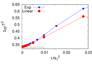
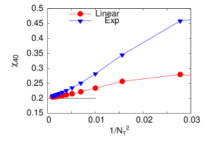
Figure 2: The second (left panel) and the fourth order (right panel) susceptibilities for free fermions as a function $1/N_{T}^{2}$ for different methods of introducing $\mu$.

The difference between the results for lattice sizes $N_{T}\leq 10$ are due to finite cut-off effects which are comparatively larger for the H-K method. This difference becomes more for the higher order QNS as shown in the plot of the sixth order susceptibility in Fig. (3).

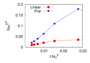
Figure 3: The sixth order susceptibility for free fermions as a function $1/N_{T}^{2}$ for different methods.

III.2 Interacting theory

In this section we compute the nth order baryon number susceptibilities at vanishing $\mu_{B}$ for two flavor QCD using staggered fermions using the operator given in Eq. (3) and the subtraction scheme explained above for the free theory. Note that we follow all the existing computations in this respect: the analytic cancellation of the divergence was shown only for the free theory and the same form used for the interacting theory. We used the same configurations used previously for estimating all susceptibilities up to the eighth order on a $N_{T}=6$ lattice gg2 . For details of the configurations and the scale setting, we refer the reader to the Ref. gg2 . The lattice size used was $24^{3}\times 6$ and the pion mass was fixed at $M_{\pi}=230$MeV, as there. The critical coupling was defined from the peak of the unrenormalized Polyakov loop susceptibility. As discussed in the Section II, the expressions of susceptibilities contain trace of fermion operator insertions. For computing each trace, 500 random vectors were used. This was also the optimum number of random vectors used in the earlier work gg1 for computation of the sixth and eighth order susceptibilities. Thus, essentially all the computational details were maintained to be the same as in gg2 . Our expressions for the various $\mathcal{O}_{n}$ are different and we use the subtraction scheme for $\chi_{20}$ and $\chi_{40}$. Our results for QNS are compared with the corresponding results of  gg2 , i.e., the exponential form and with analytic cancellation of the divergence for the free theory. Further, we also compute the ratios of our susceptibilities ans compare with the known results.

III.3 Second order

We compute the zero temperature value of $\chi_{20}$ for free fermions using Eq. (15), by numerically summing over the momentum modes on a $24^{3}$ lattice since the spatial volume for our interacting case is $24^{3}$. We then subtract this quantity from the $\chi_{20}$ values in the interacting theory computed using the $\mathcal{O}_{2}$ for our case. The left panel of Fig. (4) compares our results with those of  gg2 , labeled as ‘GG’.

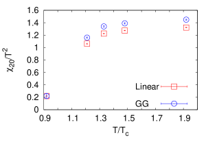
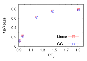
Figure 4: The second order flavor diagonal(left panel)$\chi_{20}/T^{2}$ and the corresponding one normalized by the Stefan-Boltzmann value on a $N_{T}=6$ lattice (right panel) as a function of $T/T_{c}$.

At $0.92T_{c}$, the value of our baryon number susceptibility matches with the existing GG results within errors. This suggests that including our subtracted value the of $\langle\mathcal{O}_{2}\rangle$ is effectively the same. Since the difference in the two cases comes only from the Tr$~{}\left(M^{-1}M^{\prime\prime}\right)$ for  gg2 and the subtraction term of Eq. (15) on a $24^{3}$ lattice for our case, we can infer that their values are equal within the numerical precisions. Since one is evaluated in the interacting theory while the other in the free theory, this equality justifies our ansatz that interactions do not lead to further divergent terms, as expected also in perturbation theory. Once the divergent term is subtracted the difference between the results in the two methods are due to different cut-off effects. The disagreement at the highest temperatures is consistent with the fact that there are different cut-off effects in the free theory limit i.e at asymptotically high temperatures. They would vanish only in the continuum limit or very large lattices. Again this can be easily verified by numerical computations in the free case.

We therefore check the variation of the ratio $\chi_{20}/\chi_{20,SB}$ computed as a function of temperature where the Stefan-Boltzmann(SB) value is computed on a $N_{T}=6$ lattice for both the cases. We expect that if the cut-off effects in the interacting theory are not very different from the free theory for temperatures much larger than $T_{c}$, this ratio should be independent of the subtraction procedure used. From the right panel of Fig. (4) it is evident that the GG results of  gg2 are consistent with ours for $T>T_{c}$. At $1.92~{}T_{c}$, the deviation from the Stefan-Boltzmann value is about the same($\sim 20\%$) for both the methods.

III.4 Fourth order

We follow the same subtraction procedure again for the fourth order susceptibility and compute the subtraction constant using the expression in Eq. (16) on a $24^{3}$ lattice. Comparing the $\chi_{4B}$ in the two cases in the left panel of Fig. (5), a good agreement is evident with the existing GG results. One does see, however, differences arising perhaps due to the finite size of cut-off $a=1/6T$. In the right panel of Fig. (5), the ratio of $\chi_{4B}$ and the corresponding Stefan Boltzmann value on a $N_{T}=6$ lattice is shown as a function of $T/T_{c}$. The deviations from the continuum Stefan Boltzmann value are consistent with the free theory results for $T>1.5~{}T_{c}$ indicating that the ideal gas cut-off effects are likely to be more dominant than the interaction effects. At $1.92~{}T_{c}$, the ratio is away from unity by $\sim 5\%$ in our computation whereas the deviation is about $\sim 15\%$ for the GG results. At $T=1.21~{}T_{c}$, the deviations are larger than that for free massless fermions indicating larger effects due to interactions in the medium. Of course, continuum extrapolation are needed to make prediction on the nature of the QCD medium at $T\sim 2T_{c}$, especially in view of the small differences observed.

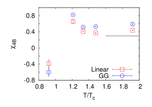
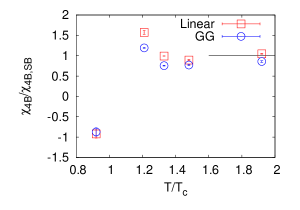
Figure 5: The fourth order baryon number susceptibility(left panel) and the same quantity normalized by the Stefan-Boltzmann value on $N_{T}=6$ lattice (right panel) as a function of $T/T_{c}$.

III.5 Sixth and higher order

For sixth order and above, we follow the lesson learnt from the free theory and do not adapt any subtraction. The sixth and the eighth order baryon number susceptibilities are displayed in Fig. (6). We find again a good agreement with the GG results. At temperatures below $T_{c}$ the larger error bars in the GG results compared to our results arise due to the presence of terms with varying sign in the former. One has larger number of matrix inversions for computing such terms and one employs noisy estimators to determine them. From the plots it is also evident that the values of the higher order susceptibilities fall to zero rapidly for $T>1.5~{}T_{c}$. The regime between $1.2-1.4~{}T_{c}$ may be still be sensitive to the critical fluctuations as seen from the large deviations of the sixth and eighth order fluctuations from the Stefan-Boltzmann values. In the continuum, the values of sixth and the higher order susceptibilities are zero for free fermions and are finite in QCD only due to the interactions. To understand how dominant are the interaction effects it is important to reduce lattice artifacts and perform a continuum extrapolation of such quantities. Using the Dirac operator in Eq. (3) these artifact effects are reduced as compared to the standard operator and also performing continuum extrapolation will be easier.

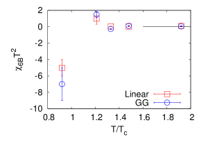
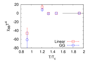
Figure 6: The sixth(left panel) and eighth order(right panel) baryon number susceptibility as a function of $T/T_{c}$.

IV Ratios of susceptibilities and Radius of convergence

The ratios of different QNS are sensitive indicators of the location of the critical point and the extent of the critical region. For massless QCD, the sixth and higher order susceptibilities should peak at $T_{c}$ with O(4) critical exponents, implying indirectly the existence of the critical point. Since our input quark mass is quite large we should expect a crossover at $T_{c}$. As mentioned in Section II, the ratios of susceptibilities are used to define the radius of convergence and hence are important for determining the location of the critical point.

Since the ratios are independent of the volume of the system, it was suggested to use them in comparisons with data a heavy ion collision experiment where it is difficult to estimate the volume of the fireball formed. Also such observables can be used for comparing lattice results at finite volume with the experiments sgupta . The ratio of the fourth to the second order baryon number susceptibility is related to the product of kurtosis($\kappa$) and square of the variance($\sigma^{2}$) of the baryon number. In the heavy ion collision experiments, the $\kappa\sigma^{2}$ of the net-proton number is measured as a function of the center of mass energy of the colliding heavy ion beams. A non-monotonic behavior of $\kappa\sigma^{2}$ as a function of beam energy is a possible signature of the existence of the critical point gg3 and is currently being probed at the RHIC mohanty .

We compute the quantity $K=\kappa\sigma^{2}$ and compare with the value of the same computed from the susceptibility values in the Ref. gg2 . Note that these are still at zero chemical potential, and are meant more for comparison of the two methods. The results are displayed in the left panel of Fig. (7). A very good agreement is observed between the results in these two different methods. This implies that the ratios of susceptibilities are not very sensitive to the subtraction scheme used. We expect that the radius of convergence estimates too would not be very sensitive to the different subtraction schemes used. In order to verify this, different radii of convergence defined in Eq. (6) were computed at $0.92T_{c}$ using our results and compared with the corresponding GG estimates. The result of the comparison is shown in the right panel of Fig. (7). As expected the radii of convergence computed using two different subtraction schemes are roughly in agreement with each other. This is promising as we can hope to now extend our analysis in the critical region with susceptibilities at tenth order and beyond this way. We hope to be able to check whether the current results on the location of the critical point are changed in a a significant way with such estimates stemming from QNS beyond the eighth order.

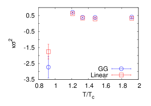
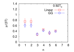
Figure 7: The kurtosis(left panel) and different radii of convergence(right panel) as a function of $T/T_{c}$.

V Conclusions

Ever since it was recognized that the lattice free theory leads to $a^{-2}$ divergences in the continuum limit, mostly the exponential form for the chemical potential term was used, as it eliminates the divergence for the free theory. Such an exponential form, however, seems not possible for the overlap quarks which have the same chiral properties as the continuum. Demanding chiral invariance for them even at finite density, one obtains an overlap operator of the form linear in $\mu$. Moreover, the linear form for any fermions, overlap or staggered, leads to simpler non-linear susceptibility expressions. Absence of canceling terms, and requirement of fewer Dirac matrix inversions make the linear form more suited for extension to higher order non-linear susceptibilities needed to estimate the radius of convergence, or the location of the QCD critical point.

In this work we proposed a numerical scheme to remove the free theory artifacts inherent in the linear form. In particular, subtractions were introduced for the second and fourth order susceptibility which we suggest should be evaluated for the free theory at zero temperature but the same spatial volume. As one sees from our Figs.  (4,5), it works well. Indeed, the main difference from the popular exponential form stem from the corresponding free theory due to the coarse finite spacing used at temperatures $T>1.5T_{c}$. For the practically more relevant ratios, such as those in the left panel of Fig. (7) used as signature for critical point or in the right panel of Fig. (7), used for estimating the radius of convergence, our method works as well as the exponential form within errors. It would be interesting to extend this work to higher orders at the critical point, estimates of which are currently obtained with susceptibilities up to the eighth order.

VI Acknowledgements

The computations were performed on the Cray X1 of the Indian Lattice Gauge Theory Initiative(ILGTI) at TIFR, Mumbai. We thank Sourendu Gupta for many helpful discussions. We would like to thank ILGTI for providing the configurations used in this work. It is a pleasure to thank Kapil Ghadiali and Ajay Salve for technical support. We gratefully acknowledge the financial support by the Alexander von Humboldt foundation and the kind hospitality of the theoretical physics group of Bielefeld University, especially that of Frithjof Karsch and Helmut Satz. The research of RVG is partially supported by a J. C. Bose Fellowship from DST. S.S. acknowledges Council for Scientific and Industrial Research for financial support during this work and thanks Saumen Datta for discussions.

References

- (1) B. Mohanty for STAR collaboration in Quark matter 2011, [arxiv:1106.5902].
- (2) V. Koch, Hadronic Fluctuations and Correlations [arxiv:0810.2520].
-
(3)
M. A. Stephanov, K. Rajagopal and E. V. Shuryak, Phys. Rev. D60,
114028 (1999);
M. A. Stephanov, K. Rajagopal and E. V. Shuryak, Phys. Rev. Lett. 81, 4816 (1998); - (4) C. R. Allton et al., Phys. Rev. D66, 074507 (2002).
- (5) C. R. Allton et al., Phys. Rev. D68, 014507 (2003).
- (6) R. V. Gavai and S. Gupta, Phys. Rev. D68, 034506 (2003).
- (7) R. V. Gavai and S. Gupta, Phys. Rev. D71, 114014 (2005).
- (8) R. V. Gavai and S. Gupta, Phys. Rev. D78, 114503 (2008).
- (9) P. Hasenfratz and F. Karsch Phys. Lett. B125, 308 (1983).
- (10) J. Kogut et al., Nucl. Phys. B 225, 93 (1983).
- (11) N. Bilic and R. V. Gavai Z. Phys. C23, 77 (1984).
- (12) R. V. Gavai, Phys. Rev. D32, 519 (1985).
- (13) R. V. Gavai and S. Sharma, Phys. Rev. D81, 034501 (2010).
- (14) R. Narayanan and S. Sharma, JHEP 1110, 151 (2011).
- (15) S. Gupta PoS CPOD 2009 025 (2009).
- (16) R. V. Gavai and S. Gupta, Phys. Lett. B696, 459 (2011).